

Abstract
Dynamic contrast-enhanced magnetic resonance imaging (DCE-MRI) has become an important tool in breast cancer diagnosis, but evaluation of multitemporal 3D image data holds new challenges for human observers. To aid the image analysis process, we apply supervised and unsupervised pattern recognition techniques for computing enhanced visualizations of suspicious lesions in breast MRI data. These techniques represent an important component of future sophisticated computer-aided diagnosis (CAD) systems and support the visual exploration of spatial and temporal features of DCE-MRI data stemming from patients with confirmed lesion diagnosis. By taking into account the heterogeneity of cancerous tissue, these techniques reveal signals with malignant, benign and normal kinetics. They also provide a regional subclassification of pathological breast tissue, which is the basis for pseudo-color presentations of the image data. Intelligent medical systems are expected to have substantial implications in healthcare politics by contributing to the diagnosis of indeterminate breast lesions by non-invasive imaging.
Keywords: Classification, clustering, computer–aided diagnosis, magnetic resonance imaging, breast
1 Introduction
Breast cancer is the most common malignant disease among women, but has an encouraging cure rate if diagnosed in an early stage. Thus, early detection of breast cancer continues to be the key for effective treatment. Dynamic contrast-enhanced magnetic resonance imaging (DCE-MRI) has become a valuable tool for detection, diagnosis and management of breast cancer [1–3]. Yet, interpretation of the multitemporal 3D image data poses new challenges to radiologists.
In DCE-MRI, multiple 3D T1-weighted magnetic resonance (MR) images of both breasts are acquired over a period of five to nine minutes while a contrast agent (CA) passes through the breast tissue. A typical sequence of images consists of one precontrast image acquired before injection of a CA bolus and a series of postcontrast images recorded afterwards over 1. Thus, a time–series signal, i.e. a vector reflecting the local signal intensities at the time points of image acquisition, is associated with each voxel. Due to characteristic changes in the structure of benign and malignant tissue influencing the flux of CA molecules between the blood pool and tissue, characteristic time–series signals can be observed for different tissue types. Interpretation of these time-series signals allows for detecting cancer with high sensitivity, even in the radio-opaque breast of young women, as well as for assessing the type of disorders in a non-invasive fashion. However, while the presence of a suspicious tissue disorder can already be identified by means of a strong signal enhancement in an early postcontrast image, the course of the entire time–series signal has to be considered for differentiating benign and malignant tissue (Figure 1) 2 [4].
Fig. 1.
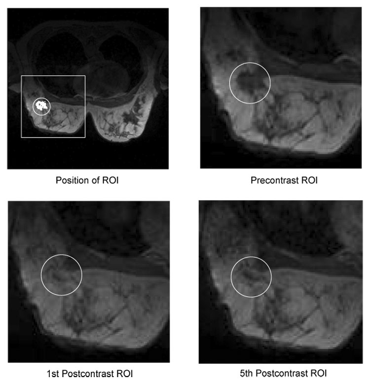
Example slices showing the enhancement of lesion tissue over time. The upper left image shows a typical field-of-view as it is used for simultaneous imaging of both breasts. The position of a region-of-interest (ROI) in the right breast is depicted by a white box. The white circle indicates the position of the lesion, which segmentation is presented in white. The remaining images show a magnified view of the ROI in the precontrast (upper right), first postcontrast (lower left) and fifth postcontrast (lower right) image. The lesion exposes a heterogeneous enhancement pattern: the intensity of the tissue in the lesion center continuously increases over time, whereas tissue at the lesion border reaches its peak intensity in the early postcontrast image and exposes lower intensity values in the late postcontrast image. These subtle differences in the temporal characteristics of the tissue are difficult to recognize in the original images but nevertheless important for the differential diagnosis of tumors.
In conventional X-ray mammography, computer-aided diagnosis (CAD) systems are being developed to expedite diagnostic and screening activities and are today moving from research to application in daily clinical practice. With breast cancer being an issue of enormous clinical importance with obvious implications to healthcare politics, much effort is spent today on research of similar techniques to aid or even automate diagnosis in breast MRI. The computer assisted interpretation of time–series signals as measured during a DCE-MRI examination for each image voxel represents one of the major steps in designing CAD systems for breast MRI. Kuhl et al. have shown that the shape of the time–series signals represents an important criterion in differentiating benign and malignant masses [4]. The results indicate that the enhancement kinetics, as represented by the time–series signals visualized in Figure 2, differ significantly for benign and malignant enhancing lesions and thus represent a basis for differential diagnosis: Plateau or washout-time courses (type II or III) prevail in cancerous tissue. Steadily progressive signal intensity time courses (type I) are exhibited by benign enhancing lesions, albeit these enhancement kinetics are shared not only by benign tumors but also by fibrocystic changes.
Fig. 2.
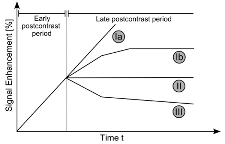
Schematic drawing of the three types of time–series signals according to Kuhl et al. [4]. Type I corresponds to a straight (Ia) or curved (Ib) line; enhancement continues over the entire dynamic study. Type II is a plateau curve with a sharp bend after the initial upstroke. Type III is a washout time course. For visual inspection, the time–series signals are typically displayed as relative-enhancement curves depicting the signal enhancement with respect to the signal intensity in the precontrast image.
Even though the time–series signals enable radiologists to infer information about the tissue state, assessing the signal characteristics is a time-consuming task which needs experience and expertise. It becomes further complicated due to the heterogeneity of lesion tissue causing the signal characteristics to vary spatially. Also these spatial variations of signal characteristics reflect specific tissue properties and should be taken into account for assessing the state of lesions. Different computerized approaches have been proposed for enhanced visualization of the multitemporal image data, facilitating the assessment of the spatio-temporal appearance patterns of lesions. Pixel-mapping functions are used to map individual time–series signals to pseudo-colors which reflect dedicated features of the temporal signal. These signal features are derived from explicit mathematical models of the time–series signals, like in the three–time–points (3TP) method [14] illustrated in Figure 3, or from more sophisticated pharmacokinetic models [16–18] describing the exchange of CA molecules between tissue compartments over time. Beside these model-based approaches, an increasing number of applications apply pattern recognition methods to extract and to visually appreciate clinically relevant information [5–11,13]. The conceptual difference between the application of pattern recognition methods like artificial neural networks or machine learning algorithms and model-based approaches is that the latter presuppose explicitly formulated models of the signal domain, while in the former implicit signal models are derived during a data-driven adaptation process from the measured data themselves.
Fig. 3.
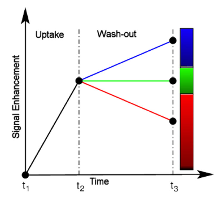
Model-based 3TP method [14,15] as the basis for pseudo-coloring of lesions voxels: the intensity of the pseudo-color represents the amount of signal uptake between the precontrast and the early postcontrast image. The presence or absence of a wash–out is associated with the color hue, yielding thus a simple lesions’ evaluation method which is capable to integrate information from exactly one precontrast and two postcontrast images.
In this article, two approaches for computing enhanced visualizations of lesions based on supervised and unsupervised pattern recognition techniques are investigated. The proposed approaches focus strictly on the observed MRI time–series signals and allow for an initially model–free and data–driven segmentation of manually marked region-of-interests (ROIs) enclosing suspiciously enhancing areas of tissue. Automatic selection of such ROIs is possible (see e.g. [26,12]), but not in the scope of this work. The time–series signals underlying the marked voxels are analyzed with respect to fine–grained differences in the amplitude and dynamics. In the supervised approach, the signals are classified by a multi-class support vector machine (MSVM) into a set of predefined tissue classes. In the unsupervised approach, a fuzzy-clustering (FC) based on deterministic annealing is applied for grouping voxels with respect to similarities between the underlying time–series signals. In either case, the outcome of the voxel-by-voxel assessment of tissue is depicted as a pseudo-color overlay e.g. in the precontrast image. Therewith, temporal and spatial tissue characteristics of individual voxels or larger segments can be observed by means of a single 3D color image.
The inspection of these pseudo-color images represents an unique practical tool for radiologists, enabling fast scans of data sets for regional differences or abnormalities of tissue enhancement and, therewith, contributes to the diagnosis of indeterminate breast lesions by non-invasive imaging.
2 Materials and Methods
2.1 Patients
A total of 12 female patients (age range with 48–61) with solid breast tumors were examined. All patients had histopathologically confirmed diagnosis from needle aspiration/excision biopsy and surgical removal. Table 1 shows the histopathologic classification and the size of the lesions for the six women with malignant tumors and six women with benign lesions.
Table 1.
Histopathologic lesion classification of the twelve cases. The lesions’ size is measured as number of voxels which have been conventionally marked by a radiologist.
| ID | Lesion classification | Size | |
|---|---|---|---|
| B1 | fibroadenoma | 169 | |
| B2 | fibrous mastopathy | 497 | |
| B3 | scar | 26 | |
| B4 | lymph node | 113 | |
| B5 | granuloma with signs of inflammation | 99 | |
| B6 | chronic mastitis | 25 | |
| M1 | DC (ductal carcinoma) | 207 | |
| M2 | scirrhous carcinoma | 49 | |
| M3 | DCIS (ductal carcinoma in situ) | 49 | |
| M4 | status post mastectomy, multilocullar recurrent DC | 169 | |
| M5 | ductal papillomatosis, transition into papillary carcinoma | 169 | |
| M6 | DC | 284 |
2.2 MR Imaging
MR imaging was performed with a 1.5 T system (Magnetom Vision, Siemens, Erlangen, Germany) equipped with a dedicated surface coil to enable simultaneous imaging of both breasts. The patients were placed in a prone position to minimize motion artifacts. Only data sets that do not require additional registration, i.e. show a suffcient anatomical alignment over time, are considered in this study. First, transversal images were acquired with a STIR (short TI inversion recovery) sequence (TR=5600 ms, TE=60 ms, FA=90°, IT=150 ms, matrix size 256×256 pixels, slice thickness 4 mm). Then a dynamic T1-weighted gradient echo sequence (3D fast low angle shot sequence, TR=12 ms, TE=5 ms, FA=25°) was performed in transversal slice orientation with a matrix size of 256×256 pixels and an effective slice thickness of 4 mm.
The dynamic study consisted of nS = 6 measurements with an interval of 110 s. The first image was acquired before injection of a paramagnetic contrast agent (Gadopentatate dimeglumine, 0.1 mmol/kg body weight, Magnevist™, Schering, Berlin, Germany) immediately followed by the 5 other measurements. The initial localization of suspicious breast lesions was performed by inspection of the subtraction image based on the first and fourth acquisition.
The following preprocessing steps are applied before evaluation of the time–series signals with one of the pattern recognition techniques: For the fuzzy clustering, each time–series signal s is transformed into a relative enhancement curve (REC), resembling the signal representation that is commonly used for manual signal evaluation in a clinical setting. The signal values are normalized with respect to the first (the precontrast) signal value s0 leading to the corresponding feature vector x ∈ X with
| (1) |
The multi-class support vector machine is applied to two different types of signal representations. Next to the unprocessed time–series signal, referred to as raw feature, the allratios feature representation is considered consisting of all possible combinations of two signal values measured at different time points.
2.3 Unsupervised Clustering of Time–Series Signals
The employed unsupervised vector quantization (VQ) algorithm – a fuzzy clustering based on deterministic annealing – is based on grouping of image voxels according to the similarity of the associated time–series signals.
Let nS denote the number of subsequent scans in a DCE-MRI study, and let nK denote the number of voxels in the marked ROIs. The time–series signals of the nK voxels, respectively their representations as RECs, can be considered as a distribution of points in a nS-dimensional feature space X. Cluster analysis groups voxels together based on the similarity of their intensity profiles in time, i.e. their Euclidean distance in X. Therewith, the entire feature space is partitioned into clusters based on the proximity of the input data. These groups or clusters are represented by prototypical time–series signals called codebook vectors (CV) located at the center of the corresponding clusters. The CVs represent prototypical time–series signals each related to a cluster of voxels sharing similar temporal characteristics.
VQ represents a fast clustering technique for feature vectors describing time–series signals in breast MRI. The cluster centers represented by the codebook vectors wi are determined by an iterative adaptive update based on the equation [19]
| (2) |
where ε(t) represents the learning parameter, ai a codebook C(t) = {wi(t)} dependent cooperativity function, κ a cooperativity parameter, and x(t) a feature vector randomly chosen at iteration t.
In this paper, a fuzzy clustering based on deterministic annealing [20,21] is employed for clustering time–series signals. Its update equation for the CVs can be derived from equation (2). The cooperativity function ai is given by
| (3) |
with ρ(t) being the time dependent ”fuzzy range” of the model, which defines a length scale in X and which is annealed to repeatedly smaller values in the course of the training. In parlance of statistical mechanics, ρ represents the temperature T of a multiparticle system by T = 2ρ2. This cooperativity function is the so–called softmax activation function, and accordingly the outputs lie in the interval [0,1] and sum up to one.
The resulting learning rule for fuzzy clustering based on deterministic annealing is given as
| (4) |
This learning rule describes a stochastic gradient descent on an error function which is a free energy in a mean–field approximation. The algorithm starts with one cluster representing the center of the whole data set. As ρ decreases during the annealing process, the VQ procedure undergoes a sequence of cluster splitting phase transitions, until a fine–grained partition of the data space is achieved. Cluster splitting occurs when a minimum of the error function (or free energy in a mean-field approximation) is transformed into a saddle point within the annealing process of the cooperativity parameter ρ. This parameter determines the amount of smoothing: for high values of ρ the clustering cost function contains only one global minimum, while for low values, the structure of the original cost function is reflected by the free energy. Thus for ρ → ∞, the free energy equals almost the original form of the clustering cost function. The repetitive cluster splitting assembles in the course of simulations a tree of codebook vectors and its resolution can be adapted according to the observer’s needs. This represents a major advantage over fuzzy c–means clustering since this algorithm does not employ prespecified number of cluster codebook vectors.
The clustering procedure identifies groups of pixels sharing similar properties of signal dynamics, and thus enables the interpretation of the physiological part of the experiment. The main differences between this method and Kohonen’s map are, as pointed in [21]: (1) the hierarchical and multiresolution aspect of data analysis, (2) monitoring based on different control parameters (free energy, entropy) facilitates straightforward cluster splitting, and (3) the learning rule based on a stochastic gradient descent on an explicitly given error function [27].
The exact number of clusters is usually determined by cluster validity techniques. In general, the higher the number the finer–grained the analyzed ROI is partitioned, however at the expense of an increase in signal noise susceptibility, while a lower number leads to an oversight of pertinent information. In our study, we have experimented with different cluster numbers ranging from 4 to 8. Our simulation results demonstrated that four clusters are adequate for a correct identification of the time–signal intensity curve types.
2.4 Classification of Time–Series Signals
In the unsupervised analysis of lesions, the grouping of time–series signals is solely determined by their distribution in X, and the diagnostic meaning of each signal cluster has to be determined after adaptation by interpreting the corresponding CVs. In contrast to that, supervised methods allow for classification of time–series signals into a predetermined set of signal classes given by a labeling of the training data by e.g. a human expert. Typically, each signal class reflects a certain tissue type or state, so that pseudo-color visualizations of the classification outcome are linked to a clear diagnostic meaning.
For the classification of DCE-MRI time–series signals we use the support vector machine (SVM) algorithm [23,22]. The SVM has been successfully applied to a wide range of classification problems and is employed for mapping DCE-MRI time–series signals to discrete class labels respectively to vectors of confidence values reflecting the probabilities of membership in the considered classes.
The basic idea of the SVM algorithm is to construct a hyperplane
| (5) |
with normal vector w ∈ X and bias b, which separates the labeled training data into two classes with maximum-margin: given a set of N labeled training examples {(x; y)i}; i = 1,…,N, xi ∈ X belonging to two different classes yi ∈ {−1, 1}, a maximum-margin hyperplane is determined which separates the training examples of the two different classes so that the distance between the hyperplane and the closest examples, the margin γ, is maximized. This hyperplane is fully specified by a subset of the training examples representing those points that lie closest to the decision surface and pose the biggest challenge in terms of classification.
Formally speaking, the margin of the hyperplane (5) is maximized by solving the following constrained optimization problem:
| (6) |
| (7) |
This optimization problem is solved by employing the Lagrange-theory, leading to the maximum-margin hyperplane normal vector
| (8) |
with αi being the Lagrange-coefficients. In practice, the decision function
| (9) |
is frequently determined by only a small subset of training examples with αi > 0, the so called support vectors, while the remaining examples with αi = 0 can be neglected.
If the two classes are not linearly separable, two modification are commonly made to the original optimization problem. First, the constraints (7) are relaxed by introducing slack variables ξi:
| (10) |
| (11) |
| (12) |
This soft-margin formulation of the support vector machine allows to tolerate a ceratin amount of margin violations, controlled by the regularization parameter C, and leads to reasonable linear classification functions even in the presence of noise or class overlap.
The second modification introduces a non-linear transformation of the data. The inner products xi · xj are replaced by a kernel function K(xi, xj) = Φ(xi) · Φ(xj), evaluating the inner product between two examples after transformation by a nonlinear function Φ(x). The hyperplane is now optimized in a new feature space and corresponds to a nonlinear decision function in the original data space. A frequently used nonlinear kernel function is the Gaussian kernel
| (13) |
In practice the regularization parameter C and the kernel bandwidth σ are varied in a wide range of values and the optimal performance is assessed on a separate validation set or using the cross-validation technique [22].
Solving multi-class problems with the SVM algorithm requires a suitable decomposition of the classification task into a sequence of binary subtasks, which each can be handled by employing the standard SVM algorithm. The outputs of the binary classifiers are then recombined to the final multi–class prediction of the multi-class SVM (MSVM).
For the classification task at hand, three different tissue classes have to be distinguished. Each tissue class is considered in one of the binary subtasks as the target class to be distinguished from the union of the remaining classes (one-vs-all decomposition scheme). The MSVM then returns three-dimensional vectors with components reflecting the outcomes of the three binary SVMs. In order to increase the interpretability of the classification outcome, it is transformed into posteriori probabilities by postprocessing with a parameterized softmax-function
The parameters are estimated by minimizing the cross-entropy error on a subset of the training data.
2.4.1 Training Data
Training examples for benign time–series signals are sampled from a set of lesions which were manually segmented by a radiologist and subsequently classified as benign according to the outcome of a histological examination. Training examples for malignant time–series signals are sampled from histologically classified malignant lesions, whereas examples for normal tissue are randomly selected from unmarked voxels. Because the histopathological classification can only be related to the entire lesion and provides no detailed information about the signal characteristics of individual lesion voxels, a certain overlap between the classes of benign and malignant training signals has to be assumed.
2.4.2 Evaluation
To evaluate the classifications of time–series signals associated with lesion voxels, a jackknife evaluation scheme is employed to the pool of 12 cases. The MSVM is adapted with a balanced set of labeled training examples sampled from eleven DCE-MRI data sets and subsequently applied for classification of time–series signals of the lesion in the excluded twelfth image sequence. This leave-one-case-out scheme is repeated twelve times so that each sequence is excluded for testing once. Pseudo-color visualizations of the excluded lesion are computed by displaying each lesion voxel with a RGB color reflecting the three-dimensional vector of posteriori probabilities resulting from the classification of the underlying time–series signal. Next to the MSVM with linear kernel function (MSVM-L), application of the MSVM with the nonlinear Gaussian kernel function (MSVM-G) is considered.
Due to the lack of a reference label reflecting the biological truth for each individual lesion voxel, the outcomes of the MSVM are compared with those of the 3TP technique, representing a clinically relevant and accepted diagnosis protocol. MSVM based visualizations are collated with those computed with 3TP, and a class label derived from the color hue assigned by 3TP to each lesion voxel serves as a ground truth for a quantitative evaluation of the MSVM based signal classification.
3 Visualization Results Based on Classification and Unsupervised Clustering Techniques
3.1 Results for Unsupervised Clustering of Time–Series Signals
In the following, we will present the segmentation method for the evaluation of time–series signals for the differential diagnosis of enhancing lesions in breast MRI.
A carefully chosen circular ROI is defined by taking into account the voxels whose intensity uptakes are above a radiologist defined threshold (> 50%) in the early postcontrast phase. The specific choice of this threshold is motivated by the relevant literature, e.g. [24], where the probability of missing malignant lesions by excluding regions with a relative signal increase of less than 50% is considered negligible. For all voxels belonging to this ROI an average time–series signal is computed. This averaged curve is then rated. This simple method is fast but is threshold–limited. A detailed analysis of the intensity curves of all voxels is then performed by the fuzzy clustering technique based on deterministic annealing as a chosen clustering method.
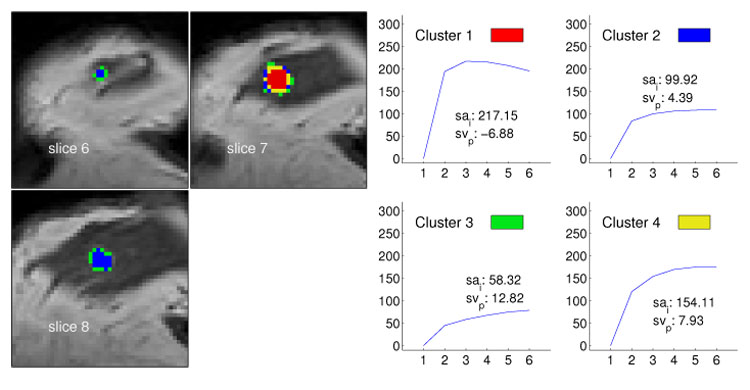
The obtained time–series signals of enhancing lesions were presented as relative enhancement curves together with the corresponding quantities initial signal change (sai), i.e., the signal change (in percent) between the precontrast and second postcontrast image, and the postinitial signal change (svp) reflecting the signal change between the third and last postcontrast image (see e.g. Fig. 4–6). The diagrams were presented to two experienced radiologists who were blinded to any clinical or mammographic information of the patients. The radiologists were asked to rate the time courses as having a steady, plateau, or washout shape – type I, II, or III, respectively [4].
Fig. 4.
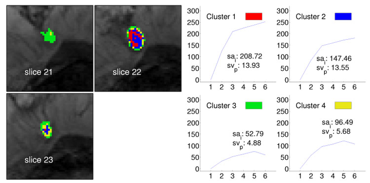
Segmentation method applied to data set B1 (benign lesion, fibroadenoma) and resulting in four clusters. The left image shows the cluster distribution for each slice ranging from 21 to 23. The right image presents for each cluster the representative time–series signal (displayed as relative enhancement curves) and the corresponding quantities initial signal change (sai) and postinitial signal change (svp). The pseudo-color images indicate strong and steady enhancing tissue in the lesion center and weakly enhancing tissue at the lesion border, suggesting an overall benign lesion.
Fig. 6.
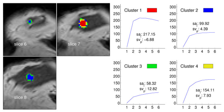
Segmentation method applied to data set M3 (malignant lesion, ductal carcinoma in situ) and resulting in four clusters. The left image shows the cluster distribution for each slice ranging from 6 to 8. The right image presents for each cluster the representative time–series signal (displayed as relative enhancement curves) and the corresponding quantities initial signal change (sai) and postinitial signal change (svp). The pseudo-color images indicate a lesion core of malignant tissue exposing signals with a strong uptake but weak wash-out. Voxels at the lesion margin expose persistently enhancing time–signal intensity curves.
The classification of the lesions on the basis of the time course analysis was then compared with the lesions definitive diagnosis. The definitive diagnosis was obtained histologically by means of biopsy or by means of follow–up in the cases that, on the basis of history, clinical, mammographic, ultrasound, and breast MR imaging findings, were rated to be probably benign.
Figure 4–Figure 6 exemplify visualizations based on the outcome of the unsupervised segmentation for one benign and two malignant lesions. The images show the cluster distribution for the given slices and at the same time the corresponding time–series signal prototype for each cluster. Thus, a very accurate representation is obtained revealing the nuances in tissue transition.
The shown images demonstrate clearly that the presented method, combining cluster analysis besides conventional method of thresholding, allows for detecting lesions and analyzing their architecture. The major advantage of the method is given by a differentiated examination of tissue changes yielding to an increase in sensitivity of breast MRI with respect to malignant lesions. Previous results of classification based either on the conventional method of thresholding or on clustering of the whole breast voxels proved to lack this capability [25].
3.2 Results for Classification of Time–Series Signals
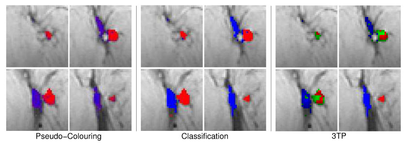
The following figures exemplify the pseudo-color visualization of manually selected ROIs using classification. Figure 7 depicts three different types of pseudo-color visualizations of the lesion of case B1. In the four adjacent image slices, only lesion voxels as marked by the radiologist are displayed with pseudo-colors. Non-lesion voxels are depicted with signal intensities of the precontrast image. In the left 2 × 2 image matrix, pseudo-colors reflect the continues values of posteriori probabilities P(classk|x) for the three tissue classes classk ∈ {malignant, normal, benigng} Thus, bright red, green and blue voxels suggest high local probabilities of malignant, normal and benign tissue, respectively. Combination of the three colors are indicative of tissue exposing time–series signals with less distinct signal characteristics. A tissue classification according to the maximum posteriori probability (red=malignant, green=normal, blue=benign) is depicted in the middle 2 × 2 matrix of images. In order to demonstrate that the MSVM based approach, although not presupposing any model assumptions about the signal, leads to a reasonable assessment of lesion voxels, the 3TP based pseudo-coloring of the lesion is displayed in the right 2 × 2 image matrix. The same types of pseudo-color images are shown for the benign case B4 and for the three malignant cases M1, M4 and M6 in Figure 8, Figure 9, Figure 10 and Figure 11, respectively.
Fig. 7.
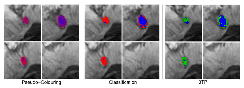
Four different image slice showing the benign lesion B1 (fibroadenoma) with pseudo-colors reflecting the local probability of malignant, benign and normal tissue (left 2 × 2 image matrix) or the local tissue classification as malignant (red), normal (green) or benign (blue) tissue (middle 2 × 2 image matrix). The 3TP based visualization of the lesion is presented in the right 2 × 2 image matrix. Both techniques indicate benign tissue (blue) in the lesion center. Tissue rated as suspicious by 3TP (green) is displayed with shadings of purple and red in the MSVM based visualization, also indicating suspicious signals with no distinct benign or malignant signal characteristics.
Fig. 8.
Same pseudo-color visualizations as described in Figure 7 but for the benign lesion B4 (lymph node). Both techniques are concordant in the assessment of benign tissue regions. Voxels of suspicious tissue (3TP: green) are displayed with shadings of purple by the MSVM.
Fig. 9.
Four adjacent image slices showing the malignant lesion M1 (ductal carcinoma) with pseudo-colors reflecting the local probability of malignant, benign and normal tissue (left 2 × 2 image matrix) or the local tissue classification as malignant (red), normal (green) or benign (blue) tissue (middle 2 × 2 image matrix). The 3TP based visualization of the lesion is presented in the right 2 × 2 image matrix. Both techniques indicate the same signal characteristics for most voxels.
Fig. 10.
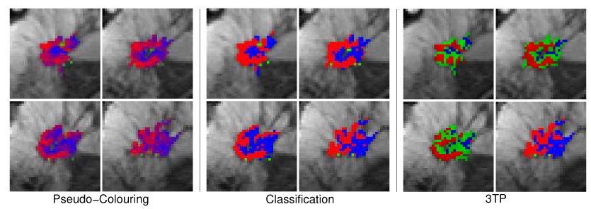
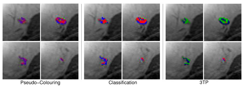
Same pseudo-color visualizations as described in Figure 10 but for the malignant lesion M4 (multilocullar ductal carcinoma). All types of pseudo–color visualizations expose the heterogenous structure of the lesion tissue, with malignant tissue areas at the lesion margin and tissue with benign signal characteristics in the core and right part of the lesion.
Fig. 11.
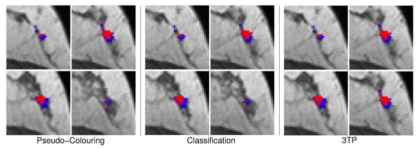
Same pseudo-color visualizations as described in Figure 10 but for the malignant lesion M6 (ductal carcinoma). Both techniques indicate two regions exposing either benign or malignant time–series signals.
The pseudo-color visualizations of all five lesion accentuate the heterogeneity of lesion tissue, stressing the requirement to analyze the enhancement kinetic of subregions of lesions instead of whole-lesion ROIs. Lesion segments with different signal characteristics can be easily identified by means of collections of voxels displayed with similar pseudo-colors.
A comparison of the pseudo-color visualizations based on the MSVM with those based on 3TP suggests a high concordance between both techniques regarding the localization of voxels exposing benign (blue) and malignant (red) signal characteristics. Tissue compartments displayed bright green by 3TP, suggesting strong uptake but indistinct wash-out characteristics of the underlying signals, are depicted purple in the MSVM based pseudo-color images.
3.2.1 Quantitative Evaluation
For assessing the classification performance of the MSVM quantitatively, the MSVM based voxel classification is compared with a reference label derived from 3TP. All voxels marked by the radiologist exhibit a significant signal enhancement and have to be regarded as suspicious lesion voxels. The marked voxels can be further subclassified into three tissue classes according to the color hue of the pseudo–color assigned by 3TP: red, blue and green voxels indicate malignant, benign and suspicious (with indistinct wash–out characteristics) time–series signals, respectively.
For the suspicious signal class of 3TP, no counterpart is provided by the MSVM. Nevertheless, to be able to assess the MSVM classification on the basis of the available ground truth, a 3 × 3 cost matrix (Table 2) is elaborated assigning a specific non-negative cost value to each pairing of 3TP (malignant, suspicious, benign) and MSVM (malignant, normal, benign) decision. The costs associated with a ”normal” classification of time–series signals by the MSVM are two, regardless of the 3TP outcome; all voxels have been marked by the radiologist as belonging to a lesion and thus have to be classified either as malignant or benign. The costs associated with the misclassification of benign as malignant and vice versa are assigned a value of one. There is zero costs if both techniques agree in their classification of signals as malignant or benign, or if a signal which is classified by 3TP as suspicious with indistinct wash–out (green) is rated as malignant or benign by the MSVM.
Table 2.
Cost matrix representing the loss associated with the different pairings of MSVM and 3TP decisions.
| MSVM | ||||
|---|---|---|---|---|
| Malignant | Normal | Benign | ||
| Malignant | 0.0 | 2.0 | 1.0 | |
| Suspicious | 0.0 | 2.0 | 0.0 | |
| Benign | 1.0 | 2.0 | 0.0 | |
For each of the twelve lesions, a 3×3 confusion matrix is computed by counting how often the different decision pairings occur. Then, the costs for classifying the lesion voxel with MSVM are determined by adding up the entries of the confusion matrix multiplied by the corresponding entries of the cost matrix. The final sum is normalized by the corresponding maximum possible cost, which is computed as the maximum entry of the cost matrix multiplied by the number of lesion voxels. The caused costs are visualized as a box plot in Figure 12. According to the medians and interquartile ranges, the best results are obtained for the MSVM–L by evaluating the raw–feature or allratios–feature representation of time–series signals. The median costs caused by classifying the twelve lesions with the MSVM-L are lower than that of the MSVM-G. Additionally, the costs for the individual lesions are much more concentrated around the medians indicating a lower inter-patient variance in the MSVM-L based cost values.
Fig. 12.
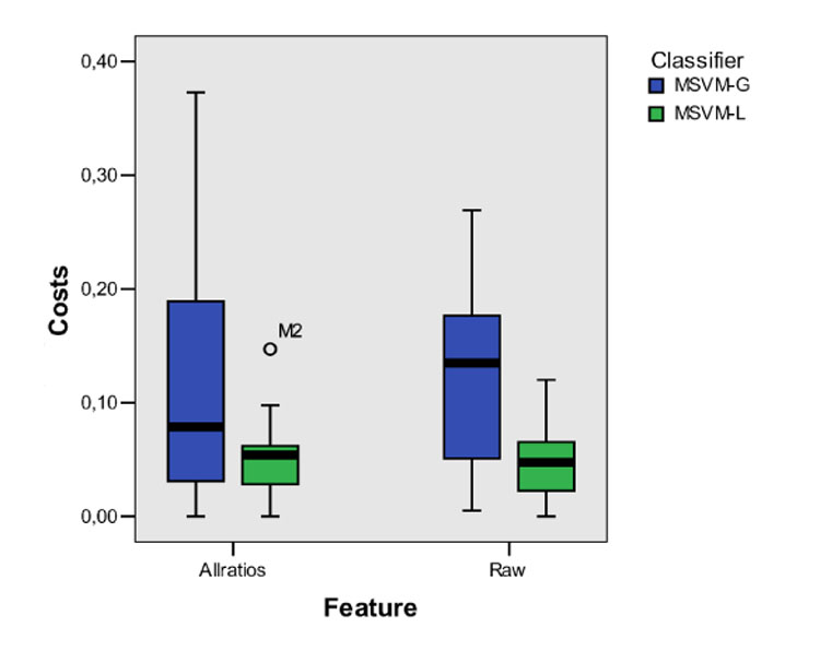
Box plot of the misclassification costs obtained for the MSVM based classification with different feature sets (raw, allratios) and different kernels (MSVM-L, MSVM G). For each combination, the median (bold line), middle half of the sample (color filled box), and extreme values (whiskers) are presented. For the MSVM with linear kernel and allratios-feature, one case deviating more than 1.5 box length from the end of the box is identified as an outlier.
The qualitative and quantitative results for the comparison of the supervised tissue classification with those of 3TP have to be interpreted with care. Even though 3TP is a clinically accepted method for analyzing lesions in DCE-MRI data sets, it does not necessarily reflect the true tissue state. Thus, it is questionable whether a perfect conformance between the MSVM and 3TP is desirable. Nevertheless, the comparison with 3TP illustrates how well the MSVM performs compared with an established and clinically applied technique. A more detailed analysis of the tissue classification requires, e.g., a histopathologically validated voxel labeling, which is difficult to obtain.
4 Conclusion and Discussion
We presented two different approaches for accentuating the spatio-temporal appearance pattern of lesions in DCE-MRI studies of breasts. Both techniques lead to visualizations of temporal image sequences in which the pseudo-color of voxels reflects the temporal characteristic of the underlying tissue. Therewith, subregions with different enhancement kinetics can be identified by means of a single 3D color image, exposing important information about the lesion architecture by the topological pattern of different tissue types in the heterogenous lesion tissue. Unlike the model-based 3TP method which only permits to consider data from one precontrast and two postcontrast images, the proposed techniques are capable of exploiting the information of the entire time–series signals. In consideration of the fact that a wide range of imaging protocols with different spatial and temporal resolutions are used in clinical practice, this flexibility with respect to the input data is a beneficial feature of the adaptive approaches.
The unsupervised approach can directly be adapted on the time–series signals of the DCE-MRI study under investigation, which avoids the requirement of a larger set of (labeled) training data. Furthermore, readaptation of the code-book vectors for each new patient allows for taking into account interpatient variabilities of the signal data caused by e.g. variations in the placement of patients in the scanner. However, the diagnostic meaning of the pseudo-colors reflecting cluster indices may vary from patient to patient, and radiologists have to interpret the codebook vectors for each case anew. At the expense of the requirement of a sufficient set of labeled training data, the pseudo-colors derived from the supervised classifier reflect definite signal characteristics. Application of both methods to patient data does not delay the diagnosis process. The training of the supervised approach with data from several labeled cases has to be executed only once, and evaluation of lesions of average size takes less than a minute. The unsupervised approach has to be retrained for each new case, but the adaptation is fast due to the typically small ROIs.
Future work will concentrate on establishing a ”digital atlas” for different lesion types as it was demonstrated in traditional digital mammography. The assessment of the morphology in addition to the temporal kinetics of lesions in a computerized fashion offers potential for substantial improvements in diagnostic accuracy and efficiency.
To extend this idea to breast MRI, we need to develop mathematical descriptors for the different morphologies, e.g., by employing shape models. Based on the combination of descriptors for the temporal and spatial tissue characteristics, we will obtain a lesion classification and also a similarity ranking within the medical image database. In summary, compact and efficient shape descriptors will improve the quality of breast MR data analysis and implicitly that of existing CAD systems beyond the current level.
Fig. 5.
Segmentation method applied to data set M1 (multilocullar recurrent ductal carcinoma) with four clusters. The left image shows the cluster distribution for each slice ranging from 13 to 16. The right image presents for each cluster the representative time–series signal (displayed as relative enhancement curves) and the corresponding quantities initial signal change (sai) and postinitial signal change (svp). The pseudo-color images indicate a lesion core of malignant tissue exposing signals with strong uptake and distinct wash-out characteristics.
Acknowledgement
The authors would like to thank Dr. A. Wismüller from the Department of Radiology, University of Munich, Germany, for providing the image data.
Footnotes
The exact number of postcontrast images and their temporal spacing depends on the imaging protocol and typically varies from clinical site to site.
Color figures are also provided in digital form in a supplemental PDF file.
Publisher's Disclaimer: This is a PDF file of an unedited manuscript that has been accepted for publication. As a service to our customers we are providing this early version of the manuscript. The manuscript will undergo copyediting, typesetting, and review of the resulting proof before it is published in its final citable form. Please note that during the production process errors may be discovered which could affect the content, and all legal disclaimers that apply to the journal pertain.
References
- 1.Yousef E, Duchesneau R, Alfidi R. Magnetic resonance imaging of the breast. Radiology. 1984 Feb;150:761–766. doi: 10.1148/radiology.150.3.6695077. [DOI] [PubMed] [Google Scholar]
- 2.Heywang S, Wolf A, Pruss E. MR imaging of the breast: Fast imaging sequences with and without Gd-DTPA. Radiology. 1989 Feb;171:95–103. doi: 10.1148/radiology.171.1.2648479. [DOI] [PubMed] [Google Scholar]
- 3.Orel SG, Schnall MD. MR imaging of the breast for the detection, diagnosis, and staging of breast cancer. Radiology. 2001;220:13–30. doi: 10.1148/radiology.220.1.r01jl3113. [DOI] [PubMed] [Google Scholar]
- 4.Kuhl CK, Mielcareck P, Klaschik S, Leutner C, Wardelmann E, Gieseke J, Schild H. Dynamic breast MR imaging: Are signal intensity time course data useful for differential diagnosis of enhancing lesions? Radiology. 1999 Feb;211:101–110. doi: 10.1148/radiology.211.1.r99ap38101. [DOI] [PubMed] [Google Scholar]
- 5.Subramaninan KR, Brockway JP, Carruthers WB. Interactive detection and visualisation of breast lesions from dynamic enhanced MRI volumes. Computerized Medical Imaging and Graphics. 2004 Aug;28:435–444. doi: 10.1016/j.compmedimag.2004.07.004. [DOI] [PubMed] [Google Scholar]
- 6.Lucht E, Delorme S, Brix G. Neural network-based segmentation of dynamic (MR) mammography images. Magnetic Resonance Imaging. 2002 Aug;20:89–94. doi: 10.1016/s0730-725x(02)00464-2. [DOI] [PubMed] [Google Scholar]
- 7.Abdolmaleki P, Buadu L, Naderimansh H. Feature extraction and classification of breast cancer on dynamic magnetic resonance imaging using artificial neural network. Cancer Letters. 2001 Aug;171:183–191. doi: 10.1016/s0304-3835(01)00508-0. [DOI] [PubMed] [Google Scholar]
- 8.Lucht E, Knopp M, Brix G. Classification of signal-time curves from dynamic (MR) mammography by neural networks. Magnetic Resonance Imaging. 2001 Aug;19:51–57. doi: 10.1016/s0730-725x(01)00222-3. [DOI] [PubMed] [Google Scholar]
- 9.Torheim G, Godtliebsen F, Axelson D, Kvistad K, Haraldseth O, Rinck P. Feature extraction and classification of dynamic contrast-enhanced T2-weighted breast image data. IEEE Transaction on Medical Imaging. 2001 Dec;20:1293–1301. doi: 10.1109/42.974924. [DOI] [PubMed] [Google Scholar]
- 10.Twellmann T, Saalbach A, Gerstung O, Leach MO, Nattkemper TW. Image fusion for dynamic contrast-enhanced magnetic resonance imaging. BMC BioMedical Engineering OnLine. 2004;3:35. doi: 10.1186/1475-925X-3-35. [DOI] [PMC free article] [PubMed] [Google Scholar]
- 11.Twellmann T, Lichte O, Nattkemper TW. An adaptive tissue characterization network for model-free visualization of dynamic contrast-enhanced magnetic resonance image data. IEEE Transaction on Medical Imaging. 2005 Dec;24:1256–1266. doi: 10.1109/TMI.2005.854517. [DOI] [PubMed] [Google Scholar]
- 12.Twellmann T, Saalbach A, Müller C, Nattkemper TW, Wismüller A. Detection of suspicious lesions in dynamic contrast-enhanced MRI data. Proceedings of EMBC 2004. 2004 doi: 10.1109/IEMBS.2004.1403192. [DOI] [PubMed] [Google Scholar]
- 13.Yoo SS, Choi BG, Han J-Y, Kim HH. Independent component analysis for the examination of dynamic contrast-enhanced breast magnetic resonance imaging data. Investigative Radiology. 2002 Dec;37:647–654. doi: 10.1097/00004424-200212000-00002. [DOI] [PubMed] [Google Scholar]
- 14.Kelcz F, Furman-Haran E, Grobgeld D, Degani H. Clinical testing of high-spatial-resolution parametric contrast-enhanced mr imaging of the breast. American Journal of Roentgenology. 2002 Jul;179:1485–1492. doi: 10.2214/ajr.179.6.1791485. [DOI] [PubMed] [Google Scholar]
- 15.Weinstein D, Strano S, Cohen P, Fields S, Gomori JM, Degani H. Breast fibroadenoma: Mapping of pathophysiologic features with three-time-point, contrast-enhanced MR imaging – pilot study. Radiology. 1999;210:233–240. doi: 10.1148/radiology.210.1.r99ja18233. [DOI] [PubMed] [Google Scholar]
- 16.Tofts PS, Brix G, Buckley DL, Evelhoch JL, Henderson E, Knopp MV, Larrson HBW, Lee T-Y, Mayr NA, Parker GJM, Port RE, Taylor J, Weisskopf RM. Estimating kinetic parameters from dynamic contrast enhanced T1-weighted MRI of a diffusible tracer: Standarized quantities and symbols. Journal of Magnetic Resonance Imaging. 1999;10:223–232. doi: 10.1002/(sici)1522-2586(199909)10:3<223::aid-jmri2>3.0.co;2-s. [DOI] [PubMed] [Google Scholar]
- 17.Hoffmann U, Brix G, Knopp MV, He T, Lorenz WJ. Pharamcokinetic mapping of the breast, A new method for dynamic MR mammography. Magnetic Resonance In Medicine. 1995 Apr;33:506–514. doi: 10.1002/mrm.1910330408. [DOI] [PubMed] [Google Scholar]
- 18.Collins DJ, Padhani AR. Dynamic magnetic resonance imaging of tumor perfusion. IEEE Engineering in Medicine and Biology Magazine. 2004 May;23:65–83. doi: 10.1109/memb.2004.1360410. [DOI] [PubMed] [Google Scholar]
- 19.Meyer-Bäse A. Pattern Recognition for Medical Imaging. Elsevier Science/Academic Press; 2003. [Google Scholar]
- 20.Rose K, Gurewitz E, Fox G. Vector quantization by deterministic annealing. IEEE Transaction on Information Theory. 1992 Mar;38:1249–1257. [Google Scholar]
- 21.Wismüller A, Lange O, Dersch D, Leinsinger G, Hahn K, Pütz B, Auer D. Cluster analysis of biomedical image time–series. International Journal on Computer Vision. 2002 Feb;46:102–128. [Google Scholar]
- 22.Cristiani N, Shawe-Taylor J. An introduction to support vector machines and other kernel-based learning methods. Cambridge Press; 2000. [Google Scholar]
- 23.Vapnik V. The nature of statistical learning theory. Springer; 1995. [Google Scholar]
- 24.Fischer U, Heyden VD, Vosshenrich I, Vieweg I, Grabbe E. Signal characteristics of malignant and benign lesions in dynamic 2D-MRI of the breast. RoeFo. 1993;158:287–292. doi: 10.1055/s-2008-1032652. [DOI] [PubMed] [Google Scholar]
- 25.Meyer-Bäse A, Wismüller A, Lange O, Leinsinger G. Computer-aided diagnosis in breast MRI based on unsupervised clustering techniques. Intelligent Computing: Theory and Applications II. Proceedings of the SPIE. 2005;5421:29–37. [Google Scholar]
- 26.Chen W, Giger ML, Bick U. A fuzzy c-means (FCM)-based approach for computerized segmentation of breast lesions in dynamic contrast-enhanced MR images. Academic Radiology. 2006;13:63–72. doi: 10.1016/j.acra.2005.08.035. [DOI] [PubMed] [Google Scholar]
- 27.Wismüller A, Meyer-Bäse A, Lange O, Schlossbauer T, Kallergi M, Reiser M, Leinsinger G. Segmentation and classification of dynamic breast magnetic resonance image data. Journal of Electronic Imaging. 2006;15(1) [Google Scholar]