Ensemble Modeling of Metabolic Networks

Abstract

Complete modeling of metabolic networks is desirable, but it is difficult to accomplish because of the lack of kinetics. As a step toward this goal, we have developed an approach to build an ensemble of dynamic models that reach the same steady state. The models in the ensemble are based on the same mechanistic framework at the elementary reaction level, including known regulations, and span the space of all kinetics allowable by thermodynamics. This ensemble allows for the examination of possible phenotypes of the network upon perturbations, such as changes in enzyme expression levels. The size of the ensemble is reduced by acquiring data for such perturbation phenotypes. If the mechanistic framework is approximately accurate, the ensemble converges to a smaller set of models and becomes more predictive. This approach bypasses the need for detailed characterization of kinetic parameters and arrives at a set of models that describes relevant phenotypes upon enzyme perturbations.

INTRODUCTION

The study of metabolic systems involves the examination and manipulation of the enzymatic reactions that make up the metabolic networks. For this reason, it is desirable to develop mathematical models of these enzymatic reaction networks to describe, understand, and eventually predict system behavior. The creation of such models allows for the generation of a set of hypotheses and a framework for further testing the capabilities of the network. However, to date, the development of detailed kinetic models (1–4) has been difficult because of the lack of kinetics, and they would be impractical for modeling large networks. The time-course data necessary to fit the parameters in these models can be difficult to obtain. Several methods have been developed to circumvent these problems and have achieved success in different aspects of metabolic modeling. These methods include the S-system approach (5,6), metabolic control analysis (7–11), stoichiometric methods (12–24) including flux balance analysis (25,26), and C13 metabolic flux analysis (27–31).

To avoid the hurdle of quantifying detailed enzyme kinetics of each reaction in the system, we focus on the use of phenotypic data, such as flux changes due to changes in enzyme expression. Even though such data are measured at steady state, they are the results of interplay among many kinetic parameters. Hence, these data provide a useful screen for kinetic models. To take advantage of these data, we first developed an approach that allowed for the construction of an ensemble of models that would all reach the given steady state in terms of flux distribution and metabolite concentrations. These models span the space of kinetics allowable by thermodynamic constraints. Once these models are constructed, they can be used to examine all possible phenotypes of the system, such as flux changes due to enzyme overexpression. When the data for flux changes due to enzyme perturbations are available, they can be used to reduce the size of the ensemble. We show that with a reasonable number of data, the ensemble converges to a model that accurately describes the system and becomes more predictive. This approach potentially circumvents the problem of acquiring detailed kinetic parameters and generates models that capture phenotypes that are dependent on kinetics, such as effects of enzyme overexpression on steady-state fluxes.

To preserve the biological mechanisms of these reactions, we model each enzymatic reaction based on the known elementary reactions, which are more fundamental than lumped kinetic models or other approximations. Our approach allows for the incorporation of details about the true mechanism of an enzymatic reaction, including regulation, but does not require such information if it is unknown. Further, by using the elementary reaction framework, we show that nonlinear saturation behavior, a fundamental property of enzymatic reactions, is intrinsically preserved. Additional information about enzyme regulation, thermodynamics, and steady-state metabolite levels can be readily incorporated into this approach.

METHODS

Obtaining steady-state fluxes

To develop a set of kinetic models that describe a given steady state, the first step is to determine the steady-state fluxes for the system. If the system has been studied previously in the literature, or is currently under study, the full flux map may have already been determined through C13 isotopomer analysis (27–31). However, this is not always the case. Often, the external fluxes of the system are known, or easily measurable. In this case, the internal fluxes of the system can be estimated by the standard flux balance around each metabolite at the steady state:

(1)

This can be represented for the entire network in matrix form:

(2)

where the matrix S is the m × n stoichiometric matrix consisting of m metabolites and n net reactions, and v is the n × 1 vector of net reactions. The steady-state metabolite concentrations are not required, but can be incorporated into the model when available. The matching of steady-state metabolite concentrations to the model will be discussed shortly.

Model building using elementary reactions

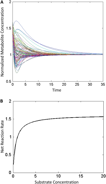
Elementary reactions are the most fundamental kinetic events at the molecular level. Each elementary reaction is either a bimolecular or unimolecular reaction that follows mass action kinetics. In our model, each enzymatic reaction is broken down into a series of elementary reactions that give the overall enzymatic reaction saturable behavior (see Fig. 2 B). This framework also allows for the simple inclusion of regulatory steps in the mechanism. In general, the mechanism for an enzyme catalyzed reaction can be represented by a collection of elementary reactions illustrated by the scheme

where the rate of each individual elementary reaction, follows the mass action principle

(3)

where is the rate constant of the forward reaction of step 1 of the overall reaction catalyzed by the enzyme i, is the concentration of metabolite i, and is the concentration of free enzyme i. By scaling the concentrations of metabolites by the corresponding concentration at the reference steady-state and those of the free enzyme and enzyme complexes by the total concentration of the corresponding enzyme at the reference state, Eq. 3 becomes

(4)

We scale by the reference states to provide dimensionless equations, which allow for easier and more accurate numerical simulations (32). This is a common practice in physics and engineering (33). Note that the rate law in Eq. 4 has the log-linear form

(5)

FIGURE 2.

(A) Example of the behavior of different models within an ensemble. All models reach the same given steady state, but all have different kinetics and thus much different dynamic behavior. Each curve represents the transient metabolite concentrations of the same metabolite from 100 models within the ensemble. The y axis is the metabolite's concentration normalized by its steady-state concentration. The time courses are generated using the network described in Fig. 3. (B) A demonstration of the elementary reaction kinetics exhibiting saturation behavior. For a single reaction, as the substrate concentration is increased, the net reaction rate reaches a maximum saturated value.

Assigning kinetic parameters

At the reference steady state, and Eq. 5 becomes

(6)

In general, if enzyme i participates in n_i elementary reaction steps, either from catalysis or regulation, there exist kinetic parameters, for rates and n_i enzyme fractions representing different complexed forms of the enzyme. These reference steady-state values are in turn constrained by

(7)

and

(8)

where is the net flux of reaction i at the reference steady state. The system is nonidentifiable, since the number of unknowns is greater than the number of equations. We must provide additional values for the enzyme fractions and n_i values related to rate i. We can assign the forward rate, which ranges from to infinity, and determine the backward rate from Eq. 8. Because the variation in the rate is large and provides no thermodynamic insight, we instead use the reversibility, defined as

(9)

where and are the forward and backward rates of step j in reaction i. Under this definition, the reversibility ranges from 0 (for an irreversible step) to 1 (for a step at equilibrium). The reversibilities of reaction steps are constrained by the Gibbs free energy of the overall reaction,

(10)

where n_i represents the number of elementary steps for enzyme i and sign(V_i,net) represents the direction of the net flux (positive if forward and negative if backward). The derivation of Eq. 10 can be found in the Appendix A. Equation 10 requires that the net flux of reaction i must be positive if and negative if We use this criterion to check whether the reference steady state is thermodynamically compliant. Furthermore, as approaches 0, this means the net reaction reaches equilibrium, and Eq. 10 implies that each mechanistic step must be at equilibrium, which satisfies the principle of microscopic reversibility (34). In reality, we know not the exact values for the Gibb free energies, but their ranges (35–37), so Eq. 10 at the reference state becomes

(11)

Different combinations of reversibilities constrained by Eq. 11 represent different kinetic states. For example, if approaches 0 while the reversibility of the other steps is near 1, then step j is rate-limiting for enzyme i. Appendix A describes in detail how we generate sets of reversibilities satisfying Eq. 11 if no other information regarding reversibilities is given.

In brief, to calculate one set of possible kinetic parameters, of each enzyme i, we first randomly assign n_i reversibilities corresponding to n_i reaction steps, and check Eq. 10 for thermodynamic feasibility. Then, the rates of the elementary reactions are determined by Eqs. 12 and 13 from the assigned reversibility and net flux:

(12)

(13)

Finally, the kinetic parameters are computed from Eq. 6 based on the corresponding rates and assigned values of enzyme fractions

Matching the steady-state metabolite concentrations

Since the kinetic equations of each elementary reaction are scaled by the reference values of metabolites at steady state, the absolute values of the metabolite concentrations need not be known. The formulation of the lumped kinetic parameter allows for simulation without the need of absolute metabolite concentrations. However, if the steady-state metabolite concentrations, are known, they can be input into Eq. 4 to solve for the individual kinetic parameter, from the lumped kinetic parameter, When this is done for all the steady-state metabolite concentrations in the system, and the set of ordinary differential equations is solved as described below, all the metabolites in the system will reach their given values at steady state.

Developing an ensemble of models spanning the kinetic space

The above process of determining kinetic parameters based on reaction reversibilities and enzyme distributions can be repeated thousands of times to develop an ensemble of kinetic models that all reach the given steady state. Each individual model can be viewed as a function of the reversibilities and enzyme fractions:

(14)

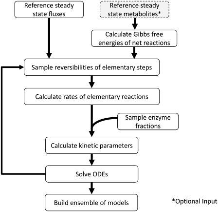
Every model reaches the same steady-state flux and metabolite concentrations, and the reversibilities and enzyme fractions are reassigned for each subsequent model. The steps that go into forming this ensemble of models are depicted in a flow chart in Fig. 1. This allows for the formation of an ensemble of models that span the range of kinetics allowable by thermodynamics, as demonstrated in Fig. 2 A. Details of how the range of kinetics is spanned are further discussed in the Results section.

FIGURE 1.

Algorithm used by the ensemble modeling framework. Note the concentrations of the metabolites at steady state are an optional input into the method.

The metabolic network for each model in the ensemble is described by a system of ordinary differential equations (ODEs):

(15)

where represents both the metabolic concentration ratios based on the reference steady state and the enzyme fractions, whereas stands for the corresponding metabolite or total enzyme concentration at the reference state. The enzyme fractions not the total enzyme concentration, now become ODE variables, and their initial conditions must be set such that

(16)

where the superscript 0 represents the initial condition of the enzyme fractions. Once the ODEs are solved, the steady-state fluxes can be readily calculated from Eq. 4 using the steady-state values for the metabolic concentration and enzyme fraction ratios.

The ensemble of models was constructed using the technical computing language MATLAB (The MathWorks, Natick, MA) on an Intel (Santa Clara, CA) Pentium 4 processor running Microsoft (Redmond, WA) Windows XP. The total computational time to develop the ensemble of models and perturb the ensemble to obtain the resulting overexpression phenotypes was ∼24 h.

Determining overexpression phenotypes

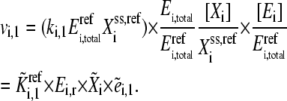
The ensemble of models developed above can be used to determine all the possible outcomes of overexpressing a particular enzyme. To do so, we perturb the entire ensemble and determine each individual model's response to enzyme overexpression, and characterize the statistical distribution of the model responses. To perturb an individual model in the ensemble, we use the equation

(17)

Equation 17 is similar to Eq. 4, but we now add an additional variable, which represents the new perturbed concentration of enzyme i. Therefore, the total enzyme ratio, represents the fold change in total enzyme concentration relative to the reference state and is an input parameter defined by the user. If the metabolic network contains any moiety conservation relationships (38), the initial conditions are set based on the reference steady state. For example, the sum of cofactors and their intermediates in the new perturbed condition must be equal to those in the reference steady state.

RESULTS

Application to central metabolism

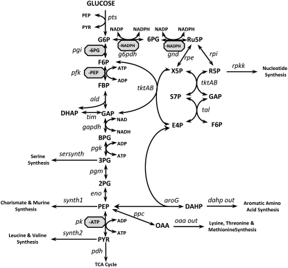
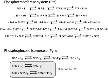
To demonstrate the applicability of our approach to metabolic modeling, we choose as a test system the primary metabolism of Escherichia coli, whose stoichiometry is detailed in Fig. 3. The structure for this system comes from the previously developed dynamic model for E. coli (4), and consists of 25 metabolite and 29 net reactions. This network contains the phosphotransferase system (Pts) for sugar uptake, glycolysis, the pentose phosphate pathway, and several branches that lead to biomass formation. Further, we have included several known inhibition reactions to demonstrate how this method can account for these inhibitory effects. An example of how the enzymatic reactions are broken down into their elementary set of reactions, and how the known mechanism of the Pts is incorporated, can be seen in Fig. 4. Also, the balancing of the cofactors (ATP/ADP, NADH/NAD, and NADPH/NADP) is taken into account in this network. As the reference state, we use fluxes taken from a previously developed dynamic model for E. coli (4). Standard Gibbs free energies for each reaction were input (37) and the thermodynamic bounds on the system were then calculated allowing for a 100-fold change in metabolite levels.

FIGURE 3.

Metabolic network of central metabolism used to test the methodology. Enzyme names are shown in italics. Metabolites are in all caps. Inhibitors are shown in gray octagons.

FIGURE 4.

Example of how the enzymatic reactions are broken down into their elementary mechanistic reactions for the phosphotransferase system (Pts) and phosphoglucose isomerase (Pgi).

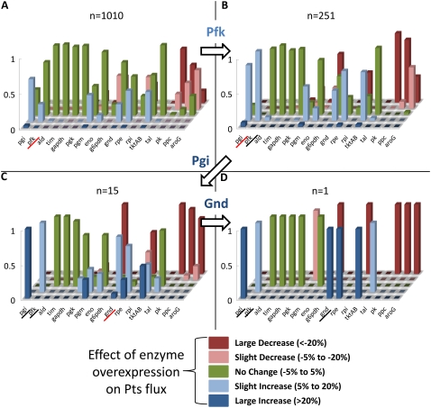
We constructed an ensemble of >1000 models (n = 1010) to span the model space. We then perturbed each internal enzyme by twofold overexpression to see the resulting change in the glucose uptake rate (the Pts flux). We grouped the resulting changes into five categories: 1), a >20% decrease in flux; 2), a decrease in flux between 5% and 20%; 3), a change within positive or negative 5%; 4), an increase in flux between 5% and 20%; and 5), a >20% increase in flux. The results of these perturbations can be seen in Fig. 5 A.

FIGURE 5.

Phenotypes of the twofold overexpression of each enzyme on the glucose uptake (Pts flux). Values are expressed as the fraction of the total number of models (n) that exhibit that phenotype. No change (green bars) indicates a change of <5% in either direction. A slight increase (light blue bars)/decrease (pink bars) indicates a change in Pts flux of between 5% and 20%. A large increase (dark blue bars)/decrease (red bars) indicates a change in Pts flux of >20%. The enzyme used for screening in each step is underscored in red. (A) The unscreened ensemble of 1010 models. (B) The screened ensemble of 251 models when Pfk is overexpressed shows a slight increase in Pts flux. (C) The second-level screening when Pgi is overexpressed gives a significant increase in Pts flux (15 models). (D) The third-level screening when Gnd is overexpressed gives a large increase in Pts flux (one model).

To demonstrate the model screening ability, we independently constructed a test model based on lumped Michaelis-Menten-type kinetics for each enzyme (39). For enzymatic reactions with more complicated mechanisms, such as the Pts for sugar uptake, the elementary reactions making up the mechanism in question were used. The steady-state fluxes for this test model were chosen to match the previously reported dynamic model of E. coli central metabolism (4). The parameters were then randomly assigned such that the test model reached the same steady state as the ensemble. This was done for the purpose of avoiding introduction of any bias in the dynamics of the test model and to keep its development completely independent from the ensemble of models. For the purpose of this demonstration, we treat the test model as the true system. The details of the test model, including how each enzymatic reaction was modeled and the assigned parameters, are discussed in more detail in Appendix B.

In the first screen, we chose phosphofructokinase (Pfk) overexpression as the first experiment since Fig. 5 A shows that Pfk is one of the enzymes that may affect the Pts flux when overexpressed. The true system was subjected to twofold overexpression of Pfk and the results showed a slight increase in the Pts flux. Therefore, in the ensemble, we retain only the models that agree with this behavior. This reduces the number of models from n = 1010 to n = 251, and the resulting behavior of the screened models is shown in Fig. 5 B.

As a second screening step, we chose phosphoglucose isomerase (Pgi) overexpression, as Fig. 5 B indicates that Pgi may be an effective target for increasing the Pts flux. Overexpression of Pgi in the true model significantly increases the Pts flux. Screening the ensemble for this behavior, we reduce the model space from n = 251 to n = 15. The result of this screening step is shown in Fig. 5 C. For the third and final screening step, we chose 6-phosphogluconate dehydrogenase (Gnd) overexpression, as this enzyme seems like a likely target to increase the Pts flux in Fig. 5 C. Overexpression of Gnd in the true model significantly increases the Pts flux. Screening the ensemble for this behavior, we reduce the model space from n = 15 to n = 1. The result of this screening step is shown in Fig. 5 D.

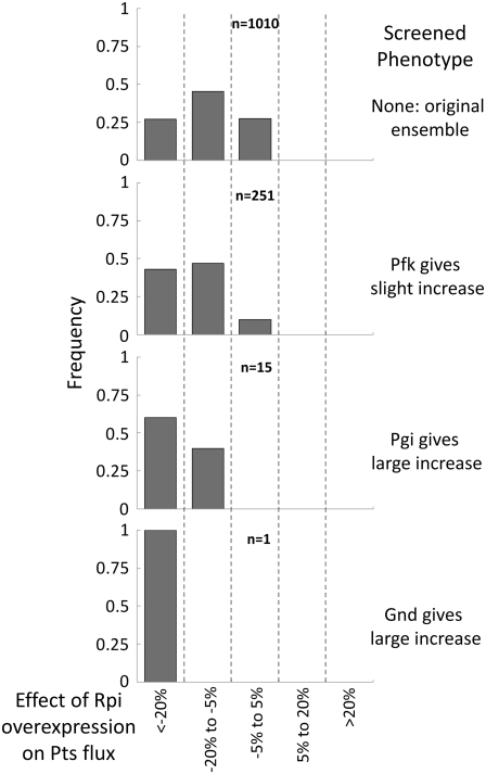
To give a close-up view of how the distribution of each enzyme's behavior is affected by this screening procedure, we can look at a cross section of the plots in Fig. 5, focusing on a particular enzyme. When we do so, we see that each subsequent screening step tightens the distribution of possible phenotypes, finally reaching a sharp peak. This is demonstrated for ribose-5-phosphate isomerase (Rpi) in Fig. 6.

FIGURE 6.

Individual view of the phenotypes for the Rpi enzymatic reaction over the same screening steps shown in Fig. 5. As the ensemble of models is screened and converges, the distribution of possible dynamic phenotypes for Rpi also converges.

Model convergence is independent of path chosen

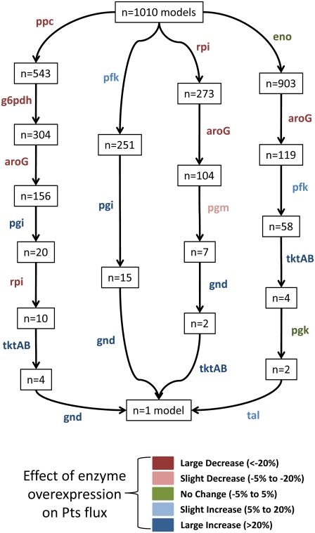
It is important to note that the single model the screening strategy converges to is independent of the data used to screen. Although screening with various phenotypic data may lead to convergence in a different number of steps, all screening paths will converge to the same model, as demonstrated in Fig. 7. This is significant, as the original distribution of predicted phenotypes in the full ensemble may suggest various enzymes for experimentation, and the screening strategy introduced here is robust, such that the convergence to a single model is insensitive to the screening path taken.

FIGURE 7.

Overexpression phenotypes chosen to screen the ensemble all converge to the same model, albeit in a different number of steps, indicating that the screening strategy is robust to the path chosen. Enzymes used for screening each step are indicated next to the appropriate arrow, and are color-coded according to their overexpression phenotype.

Behavior of the converged model

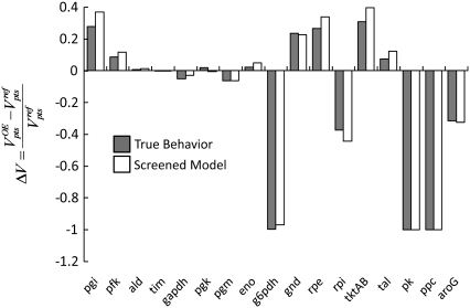
To further determine the validity of this approach, we compare the behavior of the single screened model to that of our true system. We overexpress each enzyme twofold in both the true system and our screened model, and compare the results of both models. The results of this comparison can be seen in Fig. 8. As seen from these results, the behavior of the screened model is very similar to that of the true system, indicating that the screening strategy used above is an effective way of converging to a kinetic model that accurately describes the system behavior without the need for the dedicated experiments examining each enzyme in the network to develop a detailed kinetic model.

FIGURE 8.

Comparison of the behavior of the “true” model based on individual Michaelis-Menten kinetics and the one model screened out in Fig. 5. The influence of each enzyme's twofold overexpression on the PTS flux is very similar between the true model and the model obtained through our screening strategy.

Effect of missing regulation

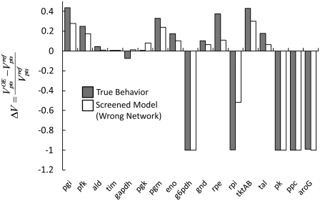
We also wish to examine how sensitive our converged model's behavior is to missing connections in the enzymatic reaction network. To test this sensitivity, we repeat the above mentioned screening steps. In this case, we input the same reaction network into the framework (Fig. 3) but remove the feedback inhibition of phosphoenolpyruvate (PEP) on the Pfk reaction. We again screen the original ensemble of n = 1010 models using the aforementioned phenotypes. If we then perturb the screened model through a twofold overexpression of each enzyme, and compare this behavior to the true model, we again see similar behavior in how the Pts flux is influenced for most of the enzymes, as shown in Fig. 9. However, we see a difference in model behavior when PGI is overexpressed, which is directly upstream and in close proximity to where the missing regulatory connection of PEP to Pfk is located. This indicates that even when the regulation of network is not completely characterized, or a connection is missed, the screened ensemble still captures much of the system behavior. Further, this presents the opportunity to identify areas of possible missing connections.

FIGURE 9.

Comparison of the behavior of the Michaelis-Menten model used as the true system and the models screened using a network with inconsistent regulatory connections. In this case, we remove the feedback inhibition of PEP on the Pfk flux in the ensemble network. Even with the inconsistent regulatory pattern between models, we see a similar behavior when each enzyme is overexpressed twofold. However, when PGI is overexpressed, we see a difference in model behavior directly upstream of the missing regulatory feature of PEP as an inhibitor to Pfk.

Spanning the kinetic space

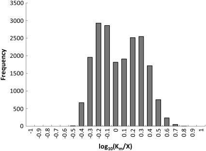
Through this scheme, an ensemble of models is generated that spans the range of all kinetics allowable by thermodynamics. Each elementary reaction is legitimately governed by mass action, which is readily formulated and linear in logarithmic scale. However, because we do so only for the elementary reactions and not for the overall enzymatic reaction, we intrinsically preserve the saturation behavior that is a fundamental property of enzymatic reactions, as shown in Fig. 2 B. This can further be shown by looking at the resulting ratio of K_m/X, where X is the steady-state concentration of the corresponding metabolite, when all the elementary steps for a given reaction are lumped together into a steady-state Michaelis-Menten form (39). We desire that the K_m values range from severalfold below the steady-state metabolite concentrations to well above this value. This would indicate that the reactions range from linear mass-action type behavior to operating at or near a saturated state. To demonstrate that the K_m values for our model system do range from well below to well above the metabolite steady state levels, we plot a histogram of the K_m/X ratios for all reactions in Fig. 10. As can be seen, some of the K_m values range from severalfold below the metabolite levels to severalfold above the steady-state metabolite concentrations.

FIGURE 10.

Histogram of log₁₀(K_m/X) values for the glycolysis model system, where X is the steady-state metabolite concentration for the corresponding metabolite. K_m values range from severalfold below the steady-state metabolite concentrations to severalfold above the metabolite concentrations, indicating that the kinetics within our system range from saturation to linear behavior.

DISCUSSION

The difficulty in developing kinetic models for metabolic systems due to lack of kinetic parameters is well recognized. Tuning a kinetic model that reaches a desired steady state is the first step of model building, but is often challenging. Here, we circumvented the problem of kinetic parameter identification by using enzyme-overexpression phenotype data, which are much more abundant and relatively easy to obtain. In doing so, we also solved the steady-state tuning problem. Our strategy constructs an ensemble of all allowable kinetic models that reach the same steady state. The ensemble is then screened using enzyme overexpression data. We show that with only a few data (three screening steps), the central metabolism model converges to the behavior of the true test model.

As one looks to expand the ensemble modeling approach to larger genome-scale systems, determining both the steady-state flux for that system and the increase in computational time required to develop an ensemble of models may become challenges that need to be overcome. The ensemble modeling approach is limited by one's access to, or ability to calculate, the reference steady-state flux of the network. As the reference flux constitutes the primary input into the algorithm, its determination may limit the scope of networks that can be examined.

In this method, the entire enzymatic network is broken down into elementary reactions rather than being composed of net reactions whose kinetics are described by the steady-state-derived Michaelis-Menten equations. The most important advantage of this formulation is that it retains the mechanistic features of enzymatic reactions, such that the resulting model can incorporate the growing knowledge of enzyme mechanisms. Second, the elementary reactions intrinsically follow mass action kinetics, which allows the log-linear formulation in Eq. 5. Third, the elementary reactions naturally give rise to the saturation behavior seen in biological systems. Further, more complicated kinetic mechanisms, such as enzyme regulation, are easily implemented into this framework through the addition of new elementary reactions. Finally, these reactions are more fundamental than lumped kinetic forms and are better posed for wide applications. These properties permit us to automate the model building procedure, allowing us to efficiently and systematically generate and test many models from the given metabolic network information. If protein expression data is available, the data can be incorporated into the framework to refine the kinetics of the ensemble to reflect the relative protein amounts present in the cell. In lieu of protein expression data, gene expression data could be used under the assumption that protein expression is roughly proportional to gene expression. If more information is given, more constraints can be applied to the models, bringing them closer to the real biological system.

APPENDIX A

In this appendix, we first derive the relationship between reversibility and Gibbs free energy described by Eq. 10 in section titled “Assigning kinetic parameters”, and then describe how to generate the reversibilities satisfying the imposed criterion. As an example, we use the same three-step reaction mechanism described in the main text:

The of the reaction i above is the ratio of the product of the forward rate constants to the product of the backward rate constants:

(18)

Since we have normalized the metabolic and enzyme concentrations by the values at the given steady state, the lumped kinetic parameter, replaces the corresponding rate constant, in the kinetic equation. For example, from Eq. 4, the lumped kinetic parameter is defined as

(19)

In a similar way, the other lumped kinetic parameters are also defined as

(20)

and

(21)

The can be expressed in terms of by substituting Eqs. 19–21 into Eq. 18:

(22)

where is the reaction quotient at the reference steady state. The first term on the righthand side of Eq. 22 reflects how far the reaction is from its equilibrium. In other words, the lumped kinetic parameters are constrained by the Gibbs free energy of the reaction at the reference steady state by the expression

(23)

where R is the universal gas constant. Next, we need to link the lefthand side of the Eq. 23 to the individual reversibilities of the elementary steps.

The reversibility defined in Eq. 9 can be written as

(24)

where sign(V_i,net) represents the direction of the net flux (positive if forward and negative if backward). If the net flux of the reference steady state is then and It is easy to see that Eq. 24 also satisfies the definition of reversibility in the opposite case, when By taking the logarithm of both sides of Eq. 24, we get

(25)

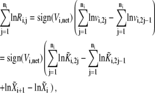
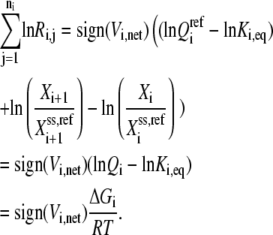
Summing up Eq. 25 for each of the elementary steps, and substituting the elementary rates as defined by Eq. 3, we get

(26)

which gives the following expression after combining Eqs. 23. and 26:

(27)

At the reference steady state, the above equation becomes

(28)

In reality, we do not know the exact values for the Gibb free energies, but their range is described by The above equality expression turns to an inequality expression represented by Eq. 11:

(11)

In general, the information regarding reversibility is often not available, so we have to generate sets of reversibilities satisfying Eq. 11 before calculating the kinetic parameters. We first check whether the direction of is thermodynamically allowable. If it is, then Eq. 11 becomes

(29)

where

(30)

and

(31)

Individual reversibilities, are generated randomly under the constraint of Eq. 29.

APPENDIX B

We constructed a test model to be used as the true system for the purpose of demonstrating the screening strategy introduced in the text. In this model, most reactions were based on lumped Michaelis-Menten-type kinetics, as indicated in Table 1. However, for the phosphotransferase system for sugar uptake, the elementary reactions making up the known mechanism were used. For reactions containing inhibition, the referenced equation forms were modified to include an inhibition term (Table 1). The transport reactions out of the system are modeled with mass-action kinetics:

(32)

TABLE 1.

List of reactions and equation forms used in test model

Reaction	Overall equation	Inhibitor	Kinetic equation
Pts	GLC + PEP → G6P + PYR	–	Elementary reactions as described in Fig. 3
Pgi	G6P → F6P	6PG	Eq. 2.15 from (39)*
Pfk	F6P + ATP → FBP +ADP	PEP	Eq. 6.2 from (39)**
Ald	FBP → DHAP + GAP	–	Eq. 33
Tim	DHAP → GAP	–	Eq. 2.15 from (39)
Gapdh	GAP + NAD → BPG + NADH	–	Eq. 6.2 from (39)
Pgk	BPG + ADP → 3PG + ATP	–	Eq. 6.2 from (39)
Pgm	3pg → 2PG	–	Eq. 2.15 from (39)
Eno	2PG → PEP	–	Eq. 2.15 from (39)
G6pdh	G6P + NADP → 6PG + NADPH	NADPH	Eq. 6.2 from (39)*
Gnd	6PG + NADP → Ru5P + NADPH	NADPH	Eq. 6.2 from (39)*
Rpe	Ru5P → X5P	–	Eq. 2.15 from (39)
Rpi	Ru5P → R5P	–	Eq. 2.15 from (39)
TktAB1	X5P + R5P → S7P + GAP	–	Eq. 6.2 from (39)
TktAB2	X5P + E4P → F6P + GAP	–	Eq. 6.2 from (39)
Tal	S7P + GAP → F6P + E4P	–	Eq. 6.2 from (39)
Pk	PEP + ADP → PYR + ATP	ATP	Eq. 6.2 from (39)**
Ppc	PEP → OAA	–	Eq. 2.15 from (39)
AroG	PEP + E4P → DAHP	–	Eq. 34
SerSynth	3PG → out	–	Eq. 32
Synth1	PEP → out	–	Eq. 32
Synth2	PYR → out	–	Eq. 32
Pdh	PYR → out	–	Eq. 32
Rpkk	R5P → out	–	Eq. 32
DAHP out	DSHP → out	–	Eq. 32
OAA out	OAA → out	–	Eq. 32
		–

Ald and AroG require modified kinetic equations because they represent one reactant going to two products (Ald) or two reactants becoming one product (AroG), which are derived from the reference used to formulate the other equations (39):

(33)

(34)

The parameter values used for the reactions are indicated in Table 2.

TABLE 2.

Kinetic parameters used in test model

Reaction	Parameter Value	Reaction	Parameter Value	Reaction	Parameter Value	Reaction	Parameter Value
Pts	K1 = 156.30	Ald	Vf = 69.91	Gnd	Vf = 75.65	Tal	Vf = 16.57
	K2 = 2000.00		Vr = 1.00		Vr = 564.17		Vr = 11.23
	K3 = 625.00
	K4 = 15.60
	K5 = 65.80
	K6 = 1.60
	K7 = 96.20
	K8 = 180.60
	K9 = 170.60	Gapdh	Vf = 671.72
	K10 = 132.30		Vr = 370.47
	K11 = 328.10					Pk	Vf = 10.17
	K12 = 41.30						Vr = 0.59
	K13 = 1010.30			Rpe	Vf = 21.05
	K14 = 3168.90				Vr = 10.62
	K15 = 870.70
	K16 = 1159.10
	K17 = 705.90			Rpi	Vf = 15.95
	K18 = 115.20				Vr = 4.31
	K19 = 63.89	Pgk	Vf = 2225.00
	K20 = 583.18		Vr = 589.80
	K21 = 973.44			TktABI	Vf = 55.57		ki = 0.64
	K22 = 17.22				Vr = 48.08	Ppc	Vf = 13.74
	K23 = 240.86						Vr = 1.41
	K24 = 137.46
Pgi	Vf = 11.09
	Vr = 0.31					AroG	Vf = 1.00
							Vr = 0.001
		Pgm	Vf = 90.55
			Vr = 6.21
Pfk	Vf = 135.66			TktAB2	Vf = 15.45
	Vr = 16.07				Vr = 2.04
		Eno	Vf = 355.79
			Vr = 4.98			SerSynth	K = 1.75
						Synth1	K = 1.41
						Synth2	K = 5.36
		G6pdh	Vf = 109.60			Pdh	K = 18.80
			Vr = 0.80			Rpkk	K = 1.03
						DAHP out	K = 0.69
						OAA out	K = 4.27
Tim	Vf = 56.87
	Vr = 38.34

References

- 1.Lee, D. Y., C. Yun, A. Cho, B. K. Hou, S. Park, and S. Y. Lee. 2006. WebCell: a web-based environment for kinetic modeling and dynamic simulation of cellular networks. Bioinformatics. 22:1150–1151. [DOI] [PubMed] [Google Scholar]
- 2.Segrè, D., J. Zucker, J. Katz, X. Lin, P. D'Haeseleer, W. P. Rindone, P. Kharchenko, D. H. Nguyen, M. A. Wright, and G. M. Church. 2003. From annotated genomes to metabolic flux models and kinetic parameter fitting. OMICS. 7:301–316. [DOI] [PubMed] [Google Scholar]
- 3.Wang, L., I. Birol, and V. Hatzimanikatis. 2004. Metabolic control analysis under uncertainty: framework development and case studies. Biophys. J. 87:3750–3763. [DOI] [PMC free article] [PubMed] [Google Scholar]
- 4.Chassagnole, C., N. Noisommit-Rizzi, J. W. Schmid, K. Mauch, and M. Reuss. 2002. Dynamic modeling of the central carbon metabolism of Escherichia coli. Biotechnol. Bioeng. 79:53–73. [DOI] [PubMed] [Google Scholar]
- 5.Savageau, M. A. 1969. Biochemical systems analysis. I. Some mathematical properties of the rate law for the component enzyme reactions. J. Theor. Biol. 25:365–369. [DOI] [PubMed] [Google Scholar]
- 6.Voit, E. O. 1991. Canonical Nonlinear Modeling: S-System Approach to Understanding Complexity. Van Nostrand Reinhold, New York.
- 7.Fell, D. A. 1997. Understanding the Control of Metabolism. Portland Press, London.
- 8.Heinrich, R., and S. Schuster. 1996. The Regulation of Cellular Systems. Chapman and Hall, New York.
- 9.Kell, D. B., and H. V. Westerhoff. 1986. Metabolic control theory: its role in microbiology and biotechnology. FEMS Microbiol. Rev. 39:305–320. [Google Scholar]
- 10.Liao, J. C., and J. Delgado. 1993. Advances in metabolic control analysis. Biotechnol. Prog. 9:221–233. [Google Scholar]
- 11.Westerhoff, H. V., and D. B. Kell. 1987. Matrix method for determining the steps most rate-limiting to metabolic fluxes in biotechnological processes. Biotechnol. Bioeng. 30:101–107. [DOI] [PubMed] [Google Scholar]
- 12.Burgard, A. P., P. Pharkya, and C. D. Maranas. 2003. Optknock: a bilevel programming framework for identifying gene knockout strategies for microbial strain optimization. Biotechnol. Bioeng. 84:647–657. [DOI] [PubMed] [Google Scholar]
- 13.Delgado, J., and J. C. Liao. 1997. Inverse flux analysis for reduction of acetate excretion in Escherichia coli. Biotechnol. Prog. 13:361–367. [DOI] [PubMed] [Google Scholar]
- 14.Famili, I., R. Mahadevan, and B. O. Palsson. 2004. k-Cone analysis: determining all candidate values for kinetic parameters on a network scale. Biophys. J. 88:1616–1625. [DOI] [PMC free article] [PubMed] [Google Scholar]
- 15.Liao, J. C., S.-Y. Hou, and Y.-P. Chao. 1996. Pathway analysis, engineering, and physiological considerations for redirecting central metabolism. Biotechnol. Bioeng. 52:129–140. [DOI] [PubMed] [Google Scholar]
- 16.Qian, H., D. A. Beard, and S. Liang. 2003. Stoichiometric network theory for nonequilibrium biochemical systems. Eur. J. Biochem. 270:415–421. [DOI] [PubMed] [Google Scholar]
- 17.Schuster, S., and I. Zevedei-Oancea. 2002. Treatment of multifunctional enzymes in metabolic pathway analysis. Biophys. Chem. 99:63–75. [DOI] [PubMed] [Google Scholar]
- 18.Segrè, D., D. Vitkup, and G. M. Church. 2002. Analysis of optimality in natural and perturbed metabolic networks. Proc. Natl. Acad. Sci. USA. 99:15112–15117. [DOI] [PMC free article] [PubMed] [Google Scholar]
- 19.Shlomi, T., O. Berkman, and E. Ruppin. 2005. Regulatory on/off minimization of metabolic flux changes after genetic perturbations. Proc. Natl. Acad. Sci. USA. 102:7695–7700. [DOI] [PMC free article] [PubMed] [Google Scholar]
- 20.Farmer, W. R., and J. C. Liao. 1997. Reduction of aerobic acetate production by Escherichia coli. Appl. Environ. Microbiol. 63:3205–3210. [DOI] [PMC free article] [PubMed] [Google Scholar]
- 21.Liao, J. C., Y. P. Chao, and R. Patnaik. 1994. Alteration of the biochemical valves in the central metabolism of Escherichia coli. Ann. N. Y. Acad. Sci. 745:21–34. [DOI] [PubMed] [Google Scholar]
- 22.Patnaik, R., and J. C. Liao. 1994. Engineering of Escherichia coli central metabolism for aromatic metabolite production with near theoretical yield. Appl. Environ. Microbiol. 60:3903–3908. [DOI] [PMC free article] [PubMed] [Google Scholar]
- 23.Patnaik, R., W. D. Roof, R. F. Young, and J. C. Liao. 1992. Stimulation of glucose catabolism in Escherichia coli by a potential futile cycle. J. Bacteriol. 174:7527–7532. [DOI] [PMC free article] [PubMed] [Google Scholar]
- 24.Patnaik, R., R. G. Spitzer, and J. C. Liao. 1995. Pathway engineering for production of aromatics in Escherichia coli: confirmation of stoichiometric analysis by independent modulation of AroG, TktA, and Pps activities. Biotechnol. Bioeng. 46:361–370. [DOI] [PubMed] [Google Scholar]
- 25.Edwards, J. S., R. U. Ibarra, and B. O. Palsson. 2001. In silico predictions of Escherichia coli metabolic capabilities are consistent with experimental data. Nat. Biotechnol. 19:125–130. [DOI] [PubMed] [Google Scholar]
- 26.Edwards, J. S., and B. O. Palsson. 2000. Metabolic flux balance analysis and the in silico analysis of Escherichia coli K-12 gene deletions. Bioinformatics. 1:1. [DOI] [PMC free article] [PubMed] [Google Scholar]
- 27.Antoniewicz, M. R., J. K. Kelleher, and G. Stephanopoulos. 2006. Determination of confidence intervals of metabolic fluxes estimated from stable isotope measurements. Metab. Eng. 8:324–337. [DOI] [PubMed] [Google Scholar]
- 28.Sriram, G., D. B. Fulton, V. V. Iyer, J. M. Peterson, R. Zhou, M. E. Westgate, M. H. Spalding, and J. V. Shanks. 2004. Quantification of compartmented metabolic fluxes in developing soybean embryos by employing biosynthetically directed fractional (13)C labeling, two-dimensional [(13)C, (1)H] nuclear magnetic resonance, and comprehensive isotopomer balancing. Plant Physiol. 136:3043–3057. [DOI] [PMC free article] [PubMed] [Google Scholar]
- 29.Sriram, G., and J. V. Shanks. 2004. Improvements in metabolic flux analysis using carbon bond labeling experiments: bondomer balancing and Boolean function mapping. Metab. Eng. 6:116–132. [DOI] [PubMed] [Google Scholar]
- 30.Yang, T. H., E. Heinzle, and C. Wittmann. 2005. Theoretical aspects of 13C metabolic flux analysis with sole quantification of carbon dioxide labeling. Comput. Biol. Chem. 29:121–133. [DOI] [PubMed] [Google Scholar]
- 31.Yang, T. H., C. Wittmann, and E. Heinzle. 2004. Metabolic network simulation using logical loop algorithm and Jacobian matrix. Metab. Eng. 6:256–267. [DOI] [PubMed] [Google Scholar]
- 32.Carr, T. W., and T. Erneux. 2001. Dimensionless rate equations and simple conditions for self-pulsing in laser diodes. IEEE J. Quantum Electron. 37:1171–1177. [Google Scholar]
- 33.Bird, R. B., W. E. Stewart, and E. N. Lightfoot. 2002. Transport Phenomena. John Wiley & Sons, New York.
- 34.Gutfreund, H. 1995. Kinetics for the Life Sciences. Cambridge University Press, Cambridge, UK.
- 35.Goldberg, R. N., Y. B. Tewari, and T. N. Bhat. 2004. Thermodynamics of enzyme-catalyzed reactions–a database for quantitative biochemistry. Bioinformatics. 20:2874–2877. [DOI] [PubMed] [Google Scholar]
- 36.Henry, C. S., L. J. Broadbelt, and V. Hatzimanikatis. 2007. Thermodynamics-based metabolic flux analysis. Biophys. J. 92:1792–1805. [DOI] [PMC free article] [PubMed] [Google Scholar]
- 37.Henry, C. S., M. D. Jankowski, L. J. Broadbelt, and V. Hatzimanikatis. 2006. Genome-scale thermodynamic analysis of Escherichia coli metabolism. Biophys. J. 90:1453–1461. [DOI] [PMC free article] [PubMed] [Google Scholar]
- 38.Kholodenko, B. N., M. Cascante, J. B. Hoek, H. V. Westerhoff, and J. Schwaber. 1998. Metabolic design: how to engineer a living cell to desired metabolite concentrations and fluxes. Biotechnol. Bioeng. 59:239–247. [DOI] [PubMed] [Google Scholar]
- 39.Cornish-Bowden, A. 1979. Fundamentals of Enzyme Kinetics. Butterworths, London.