The Poisson-Boltzmann model for tRNA

Abstract

Using tRNA molecule as an example, we evaluate the applicability of the Poisson-Boltzmann model to highly charged systems such as nucleic acids. Particularly, we describe the effect of explicit crystallographic divalent ions and water molecules, ionic strength of the solvent, and the linear approximation to the Poisson-Boltzmann equation on the electrostatic potential and electrostatic free energy. We calculate and compare typical similarity indices and measures, such as Hodgkin index and root mean square deviation. Finally, we introduce a modification to the nonlinear Poisson-Boltzmann equation, which accounts in a simple way for the finite size of mobile ions, by applying a cutoff in the concentration formula for ionic distribution at regions of high electrostatic potentials. We test the influence of this ionic concentration cutoff on the electrostatic properties of tRNA.

1 Introduction

Due to its long-range nature, electrostatic interactions play a key role in determining the structural and dynamical properties of biomolecules, as well as in characterizing their association processes. Because the interactions between charged molecules are affected by the presence of water and salt, in the studies of biomolecular encounter, one of the important aspects is proper description of the electrostatic potential around the molecule in various environments. For many years the Poisson-Boltzmann (PB) theory has been used for this purpose (see e.g. [1, 2, 3, 4]). In the PB model a molecule is represented as a set of spheres with partial atomic charges immersed in implicit solvent with diffuse ions represented by Boltzmann distribution. Both charge distributions appear in the PB equation which is numerically solved on a 3D grid to determine the electrostatic potential around the molecule. Even though the formalism of the PB theory and its application to biological molecules are nowadays well documented, see e.g. [5, 6], the PB model still suffers from many limitations. Some of those limitations arise from the fact that it is a mean-field like theory and others result from the calculation setup. The setup often makes use of a single conformation of the solute which does not account for the dynamic reorganization of atomic charges. Other draw-backs result from sensitivity to the choice of parameters such as, for example, dielectric constant, partial charges, van der Waals radii, and the placement of the dielectric boundary between the solute and the solvent. Also, the quality of the crystal structure can affect the results of the PB calculations.

In this work, we discuss some of the setup type limitations but we also focus on those arising from the standard PB theory itself. Those theory-inherent limitations include, for example, the fact that the Boltzmann distribution does not account for the finite size of ions and this can lead to overestimation of ionic concentrations close to molecular surfaces. Moreover, size dependent ion-ion correlations and fluctuation contribution to the ion distributions are not taken into account what results, for example, in the inability of the PB theory to predict attraction between the equally charged surfaces [7, 8]. The importance of ionic size was evidenced experimentally, e.g. in the studies of RNA folding in the presence of divalent cations, and the results were qualitatively confirmed by Brownian dynamics simulation with explicit representation of ions [9].

The overall strengths of the PB theory include the fact that after calibration of parameters many types of simulations can be performed at modest costs of the computer power only. Usually, for macromolecular complexes very sophisticated methods such as thermodynamic integration and Monte Carlo simulations are not computationally feasible.

Even though there are numerous examples including ours [10, 11, 12] where even the linear approximation to the solution of the PB equation for highly charged large biomolecules was successful, those kinds of solutes may require modifications of the PB model to account for the finite size of ions to eliminate nonphysically high concentrations close to their charged surfaces. Such modification of the PB equation was proposed before in the theory of Borukhov and co-workers which was based on the lattice gas formalism but it was applied to model geometries [13, 14]. An extension of the Borukhov model accounting for various sizes of ions was recently proposed in [15]. A more advanced modified PB theory based on the exact statistical theory of ionic solutions and the so-called Kirkwood charging method is also well established [16, 17, 18, 19] (see also reviews [20, 21] and references therein). In this theory the Boltzmann ionic distribution is corrected with the so-called exclusion volume term (accounting for short range van der Waals interactions of ions) and with an additional electrostatic fluctuation term. However, the latter approach is computationally very expensive and applications to realistic macromolecular systems are so far very limited [22]. It is also possible to combine the PB model applied to ions in the solvent surrounding a molecule with an explicit description of ions bound to the molecule. The latter ions can be treated with a tightly bound ion (TBI) model which provides an approximate statistical distribution of ions in cells representing the bound regions on the molecular surface and automatically accounts for the ionic size [23].

First, our studies aim at testing the sensitivity of the electrostatic potential around the tRNA molecule to various conditions of the surrounding, e.g., to the presence of explicit divalent ions and their coordinating water molecules. Electrostatic potential around the tRNA molecule with a nonlinear PB model was shown in [24, 25, 26] but the effect of crystallographic water molecules and divalent ions was not discussed.

Second, we evaluate the sensitivity of the electrostatic potential and the electrostatic free energy resulting from the PB theory to introduction of the finite size of diffusely bound ions. In a very simple approach, we approximate this effect by imposing an upper limit on the value of concentration of ions resulting from the Boltzmann expression.

For both aims, we chose to perform analysis on the tRNA molecule [27]. Due to its moderate size and negative net charge it is a very good object for numerous tests of the PB model, its limitations, as well as modifications. To compare the electrostatic potential around tRNA, we apply various similarity measures such as Carbo index [28] and Hodgkin index [29] (HI) or simply a root mean square deviation (RMSD). The results obtained for the tRNA molecule will allow us to determine the most reliable conditions and calculation setup for future studies on highly charged macromolecules such as the ribosome.

2 Methods

2.1 The system

Yeast phenylalanine tRNA crystal structure, solved to a resolution of 1.93 Å (1ehz PDB entry), was used in the simulations. It contains 9 divalent ions - six Mg²⁺ ions and three Mn²⁺ ions - coordinated by a total of 35 water molecules (the structure is labeled as t9w and presented in Figure 1).

Figure 1.

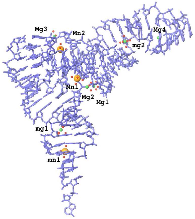
Heavy atom model of tRNA (blue sticks) with crystallographic divalent metal ions (magnesium in green, manganese in orange) surrounded by oxygen atoms of coordinating water molecules (red dots). Labels correspond to ionic names presented in Table II. The most solvent exposed ions, which are not present in t6 and t6w systems, are designated by small letters.

To determine whether the crystallographically resolved tightly bound divalent Mn²⁺ and Mg²⁺ ions could be replaced in electrostatic calculations by the Boltzmann distribution of “continuum” ions, simulations for various pairs of tRNA systems were compared for the t9w structure and a set of other systems, labeled t9, t6w, t6, t6wb, t6b and t (a digit defines the number of explicit ions in the tRNA system and w denotes their coordinating crystal water molecules). The t9 structure is obtained by removing all the coordinating water molecules from the t9w structure, the t6w structure is the result of deleting the three most exposed to solvent metal ions (two Mg²⁺ and one Mn²⁺ which were located outside ion’s exclusion layer) together with their 16 coordinating water molecules. The deletion of the rest of the water molecules yields the t6 structure. The t6wb structure is obtained by the removal of 3 Mg²⁺ ions with highest water coordination number (a total of 17 water molecules). Again, deletion of the rest of the coordinating water molecules yields t6b. These b labeled structures were included to compare the potentials derived for different ion binding modes. By ion binding mode we define a manner in which a given ion binds to tRNA: directly (no mediating waters), through one water molecule (sharing their solvation shells with tRNA’s solvation shell) or through two water molecules (ion surrounded by its solvation shell binds to tRNA’s solvation shell) [30]. Finally, the t structure stands for a bare tRNA with all the metal ions and water molecules removed. Summary of the structures used in this study is shown in Table I. The information which crystal ions were removed together with their distance to the tRNA is presented in Table II.

Table I.

Labels for tRNA systems giving the number of crystallographic ions and coordinating them water molecules and the net charge (in e) of the system

Label	#ions	#H2O	net charge
t9w	9	35	-56
t9	9	none	-56
t6w	6	19	-62
t6	6	none	-62
t6wb	6	18	-62
t6b	6	none	-62
t	none	none	-74

Table II.

Description of crystallographic ions in each of tRNA systems

Ion name	tRNA systema	NH2Ob	NtRN Ac	dH2OdÅ	dtRN AeÅ
mg1	t9, t9w	5	0	2.005	-
mg2	t9, t9w	6	0	2.006	-
Mg1	t9, t9w, t6, t6w	6	0	2.006	-
Mg2	all except t	1	2	2.005	1.929,2.599
Mg3	all except t	3	1	2.005	2.066
Mg4	all except t	0	3	-	2.53, 3.0, 3.09
mn1	t9, t9w, t6b, t6wb	5	1	2.015	2.296
Mn1	all except t	5	1	2.016	2.470
Mn2	all except t	4	1	2.019	2.182

^alabels for tRNA structures in which certain ion name or water molecules are present.

^bnumber of water molecules coordinating an ion.

^cnumber of close contacts (< 2.6 Å except for Mg4) between ions and tRNA.

^dmean distance between an ion and oxygens of coordinating water molecules.

^eion-closest tRNA atom distance (enumerated in column N_tRNA).

2.2 Poisson-Boltzmann equation

To calculate the electrostatic potential with the Poisson-Boltzmann model, the system under study is divided into two regions: interior of the solute molecule characterized with a low dielectric constant and with fixed distribution of atomic point charges and radii, and the external continuous environment characterized with high dielectric constant of water and concentrations of diffusive ions typical for the physiological environment.

The electrostatic potential, ψ(r), is then calculated from the PB equation which describes the potential arising from the fixed charge distribution of solute point charges, ρ^fix(r), and Boltzmann distribution of mobile ion charges in the surrounding dielectric medium:

$$\nabla \cdot [\epsilon \left(\mathbf{r}\right)\nabla \psi \left(\mathbf{r}\right)]+4\pi {\rho }^{\mathit{fix}}\left(\mathbf{r}\right)+4\pi \lambda \left(\mathbf{r}\right)\sum _{i}e{z}_i{c}_i^b\exp (-\beta e\psi \left(\mathbf{r}\right)z_i)=0.$$ (1)

The sum on the left hand side represents the Boltzmann distribution of i ionic species, β equals 1/k_BT, e is the charge of an electron, z_i and $c_i^b$ are the valence number and bulk concentration of ith ion species, respectively. The dielectric constant, ε(r), and the ion-accessibility parameter, λ(r), are region dependent. The latter parameter is equal to 1 in the regions accessible to ions, and 0 elsewhere (see also discussion in the first paragraph of sec. 2.5).

The potential resulting from the PB equation represents a stationary point of a functional,

$$G\left[\psi \right]=\int \left[-\frac{\epsilon }{8\pi }{(\nabla \psi )}^2+{\rho }^{\mathit{fix}}\psi -{\beta }^{-1}\lambda \left(\mathbf{r}\right)\sum _i{c}_i^b(e^{-\beta e{z}_i\psi }-1)\right]{\mathrm{d}}^3\mathbf{r},$$ (2)

which is interpreted as the electrostatic free energy of the system [5]. The three terms of the integral are sometimes referred to as dielectric (G^diel), fixed charge (G^fix) and mobile charge (G^mob) contribution, respectively, so that G = G^fix-G^diel-G^mob (see the on-line documentation of APBS software or [31]).

For small electrostatic potentials, ψ, eq. 1 may be simplified by expanding the mobile ion distribution term in the Taylor series and keeping only the linear terms. Assuming that the total charge concentration in the bulk solvent is zero, i.e., ${\sum }_i{z}_i{c}_i^b=0$ the linearized PB equation takes the form:

$$\nabla \cdot [\epsilon \left(\mathbf{r}\right)\nabla \psi \left(\mathbf{r}\right)]+4\pi {\rho }^{\mathit{fix}}\left(\mathbf{r}\right)+4\pi \beta \lambda \left(\mathbf{r}\right)\sum _i{e}^2{z}_i^2{c}_i^b\psi \left(\mathbf{r}\right)=0$$ (3)

One often defines ionic strength through ionic concentrations c_i and charge numbers z_i of constituting ions as $I=\frac{1}{2}{\sum }_i{c}_i{z}_i^2$.

The free energy functional corresponding to the linear PB equation can be obtained from eq. 2 by expanding the exponential expression into Taylor series and keeping the lowest non-vanishing, quadratic term. It can be shown that the stationary value of that functional is simply (compare with [1]),

$$G^{\mathit{lin}}=\frac{1}{2}\int {\rho }^{\mathit{fix}}{\psi }^{\mathit{lin}}{d}^3\mathbf{r}$$ (4)

where ψ^lin denotes the solution of linearized form of the PB equation. Because the higly charged tRNA yields strong electrostatic potential close to its molecular surface, this system might not be properly described with the linearized PB equation. Therefore, in few cases we compared the results obtained with linear and nonlinear PB equations. In particular, we determined the energetic effect of linearization,

$$\Delta G^{\mathit{lin}}=G^{\mathit{lin}}-G.$$ (5)

2.3 Application of ionic concentration cutoff

In the PB model, the Boltzmann distribution for mobile ions does not account for their finite size and this may lead to unphysically high concentrations of counterions near charged molecular surfaces. Different modified PB models accounting for the finite size of ions are discussed in detail elsewhere [20, 32, 33]. In this study, we test the most simple approach in which we ignore the competition of different ionic species so that the concentration of each species can be independently corrected for its maximum concentration $c_i^{\mathit{max}}$ (further referred to as the cutoff),

$$c_i^{\mathit{cut}}\left(\mathbf{r}\right)=\min \{c_i^b{e}^{-\beta e{z}_i\psi \left(\mathbf{r}\right)},c_i^{\mathit{max}}\}.$$ (6)

Ignoring the competition beetween different ionic species in the cutoff (eq. 6) is justified if there are only one cationic and one anionic species in solution or if possible additional species are represented as explicit site-bound ions, like the crystallographic magnesium.

Another problem behind eq. (6) is the fact that if ions are modeled as hard spheres with point charges in their centers, there is no upper limit on the value of mean ionic concentration in a single point of space. In this case, a true cutoff condition (still ignoring the competition of ionic species) is,

$${\int }_{V\mathbf{r}}{c}_i({\mathbf{r}}^{\prime }{d}^3{\mathbf{r}}^{\prime }\le 1)$$ (7)

where V_r denotes a sphere with a center in an arbitrary point r and with radius a_i. The diameter of the sphere, 2a_i, determines the distance of the closest approach between the ion centers. The parameter a_i can be assumed as the van der Waals radius of a bare ion but one can also consider the radius of an ion with its first solvation shell. Implementation of inequality (7) would be, however, very difficult. Therefore, we investigated the possibility of using eq. (6) with parameter $c_i^{\mathit{max}}$ adjusted in an empirical way, so as to qualitatively reproduce condition (7). One can expect that reasonable values of $c_i^{\mathit{max}}$ are in the range from $1∕(4\pi a_i^3∕3)$ to 1/δ³ where δ < a_i is the spatial resolution of the grid used for discretization of ionic concentrations and the potential in the finite difference method. Unfortunately, the upper limit 1/δ³ is not very useful in our case, because we use a dense grid. A similar simple approach for ionic concentration cutoff was applied in [32] for a planar-double layer problem. In that study c^max = 1/a³, where a was interpreted as the diameter of the ion and set to 3Å.

In case of nucleic acids one has to take into account that the distribution of ions near a molecular surface is non-uniform and the cutoff value, $1∕(4\pi a_i^3∕3)$, is too restrictive. Therefore, we use

$$c_i^{\mathit{max}}=\frac{\alpha }{\frac{4}{3}\pi a^3},$$ (8)

where α ≥ 1 is an empirical scaling parameter. From the requirement that the excess number of ions derived from the cutoff condition (6),

$$\Delta n_i^{\alpha }=\int [c_i\left(\mathbf{r}\right)-c_i^{\mathit{cut}}\left(\mathbf{r}\right)]d^3\mathbf{r},$$ (9)

is equal to the excess number of ions derived from the condition (7),

$$\Delta {\stackrel{‒}{n}}_i=\frac{V}{{\Sigma }_{\mathbf{r}}{V}_{\mathbf{r}}}\sum _{\mathbf{r}}[{\int }_{V_{\mathbf{r}}}{c}_i\left({\mathbf{r}}^{\prime }\right)d^3{\mathbf{r}}^{\prime }-1]$$ (10)

we find an optimal value for α. The above expressions are evaluated for ionic distribution c_i resulting from the solution of the conventional nonlinear PB equation. In (10) the sum runs over those points r of the grid for which condition (7) was violated. V denotes the total ion-accessible volume covered by the spheres V_r, and the fraction V/ΣV_r is used in eq. (10) to account for the partial overlap of spheres.

Applying the cutoff expressions (6) and (8) in place of the Boltzmann distribution in eq. (1) we obtain a modified nonlinear PB equation. The corresponding modified expression for the electrostatic free energy takes the form,

$$G^{\mathit{cut}}=G^{\mathit{fix}}-G^{\mathit{diel}}-{G^{\mathit{mob},}}^{\mathit{cut}},$$ (11)

where the components G^fix and G^diel are the same as in the conventional expression for the free energy (2), and

$${G^{\mathit{mob},}}^{\mathit{cut}}={\beta }^{-1}{\int }^{\prime }\left[\sum _i\min \{c_i^b(e^{-\beta e{z}_i\psi }-1),-\beta e{z}_i\psi c_i^{\mathit{max}}+B_i\}\right]{\mathrm{d}}^3\mathbf{r}.$$ (12)

The prime in the above expression indicates that integration is performed only in the ion-accessible region. A constant, B_i, ensures that truncation of the energy functional (12) and truncation of the concentration (6) become effective for the same threshold value of the potential ψ,

$$B_i=c_i^{\mathit{max}}\left(1-\ln \frac{c_i^{\mathit{max}}}{c_i^b}\right)-c_i^b.$$ (13)

The effect of the cutoff is expressed with an energy difference

$$\Delta G^{\mathit{cut}}=G^{\mathit{cut}}-G$$ (14)

where G^cut and G are the electrostatic free energies obtained with and without the concentration cutoff correction, respectively. It is interesting to compare the energetic effect of the cutoff with the energetic effect of linearizing the PB equation (5) (see Section Results).

We also calculated the influence of ion concentration cutoff on the free energy differences between systems immersed in media with different ionic strengths. For this purpose we define a change in the free energy difference, ΔΔG:

$$\Delta \Delta G^{\mathit{cut}}=\Delta G_{n2}^{\mathit{cut}}-\Delta G_{n1}^{\mathit{cut}},$$ (15)

where n2 and n1 denote different mobile ionic compositions (see Table III). The above equation can be rewritten,

$$\Delta \Delta G^{\mathit{cut}}=\Delta G_{n2n1}^{\mathit{cut}}-\Delta G_{n2n1},$$ (16)

where ΔG_n2n1 = ΔG_n2 - ΔG_n1 and $\Delta G_{n2n1}^{\mathit{cut}}=G_{n2}^{\mathit{cut}}-G_{n1}^{\mathit{cut}}$, are electrostatic free energies of introducing additional ionic species into solvent. Then ΔΔG^cut is simply a change in ΔG_n2n1 upon applying the concentration cutoff.

Table III.

Ionic concentrations (c) and resulting ionic strengths (I) used in the linear (l) and nonlinear (n) PB calculations

Label	cNa+	cCl	cMg2+	I
l1	0.15a	0.15	-	0.15
l2	0.15	0.19	0.02b	0.21
n1	0.15	0.15	-	0.15
n2	0.15	0.19	0.02	0.21

^aphysiological concentration of Na⁺;

^bphysiological concentration of Mg²⁺ (including bound ions) as given by e.g. [42];

In all reported relative free energies, ΔG was calcuated between the systems having the same number of explicit crystallographic ions and water molecules. To compare systems having different number of crystallographic ions we use the differences in ΔG (ΔΔG). This way we avoid comparing large values of absolute solvation free energy.

2.4 Numerical solution

Hydrogen atoms were added to the tRNA molecule using the Amber [34] force field and package and their positions were energy minimized with 8·10³ steps of steepest descent minimization method followed by 2·10³ steps of conjugate gradients method.

All solutions of the PB equation were obtained with the Adaptive Poisson-Boltzmann Solver (APBS) [31] and the finite-difference technique using the multigrid solver [35]. We chose to analyze the electrostatic potentials for two different ionic compositions (with and without Mg²⁺ ions) which are commonly used in the electrostatic calculations and whose monovalent and divalent ionic concentrations correspond to physiological conditions. The notation and parameters used in the calculations are gathered in Table III. The linear and nonlinear PB calculations in the NaCl solution will be further referred to as l1 and n1, respectively. By analogy, l2 and n2 will denote the linear and nonlinear PB calculations in the solution including both NaCl and MgCl₂.

Electrostatic grid dimensions were set to 102 × 90 × 128 ų, with the grid center located in the geometric center of the t9w system, and the solution of the PB equation was obtained to a grid resolution of 0.4Å. Multiple Debye-Hückel boundary conditions were used [36]. The dielectric constant of each solute was assigned a value of 2 and that of the solvent of 78.54, the temperature was set to 298 K (these are default values in APBS software). The solute-solvent dielectric boundary was defined by the molecular surface using a probe sphere radius of 1.4 Å. The diffuse ion exclusion radius was set to 2.0Å. The crystal Mn²⁺ and Mg²⁺ ions were assigned a radius of 2.34 Å, in accord with the applied force field. Each of the l1, l2, n1 and n2 calculation schemes was applied to each of the tRNA systems shown in Table I.

2.5 Analysis

The analysis was based on the electrostatic potentials and electrostatic free energies obtained from APBS. To compare the results as a function of the distance from the tRNA surface, we applied an approach based on inflating the van der Waals surface. The inflated vdW surface (or ion accessible surface) is created by enlarging the vdW surface by a given radius. When the radius is set to zero, one obtains the vdW surface of a molecule. By increasing the ionic radius from 0 by 1Å for 10 consecutive steps, we generated ten surfaces around tRNA.

Surface potential maps were obtained by mapping the electrostatic potential onto consecutive ion accessible surfaces (using OpenDX IBM’s Visualization Data Explorer) of the t9w system. The choice of a common surface for potential maps of all systems ensures that the comparisons are made in the same point of space. The t9w surface was chosen because being the largest one it prevents from mapping the potential of the inside of the molecule for other tRNA systems.

Electrostatic potentials were compared using similarity indices: potential RMSD, residual function [37] (RF), and Hodgkin index [29] (HI).

$${\mathit{RMSD}}_{A∕B}={\left[\frac{1}{N}\sum _{i=1}^N{(A_i-B_i)}^2\right]}^{1∕2}$$ (17)

$${\mathit{RF}}_{A∕B}=\frac{1}{N}\sum _{i=1}^N\frac{\mid A_i-B_i\mid }{\mid A_i\mid }$$ (18)

$${\mathit{HI}}_{A∕B}=\frac{2\sum _{i=1}^N{A}_i{B}_i}{\sum _{i=1}^N{A}_i^2+\sum _{i=1}^N{B}_i^2}$$ (19)

where A_i and B_i are the potential values, and the sums run over points of either the exterior of the molecule or a surface map.

We also tested Tanimoto [38] and Carbo [28] indices. However, they gave redundant results - Tanimoto index yielded qualitatively identical results as HI and Carbo index gave large and unnormalized results diffcult to interpret but qualitatively similar to those from RMSD comparisons.

3 Results

Two types of comparisons of the electrostatic potential around tRNA were carried out. The first one, was between the electrostatic potential of different tRNA systems - any of t, t6, t6w, t6b, t6wb, t9, t9w (Table I) - calculated using the same form of the PB equation and the same PB parameter set-up (Section 3.1). The second type was between the electrostatic potential calculated for a single tRNA system but with different forms of the PB equation (linear or nonlinear) and/or different ionic strength (Table III, Section 3.2). Additionally, the effect of the ionic concentration cutoff on the results of the PB calculations was tested and is presented in Section 3.3.

3.1 Comparison of electrostatic potential of different tRNA systems

Figure 2 presents HI and RF indices calculated for different pairs of tRNA systems and over those grid points which exclude the molecular interior. Results are shown for both forms of the PB equation, as well as two ionic strengths. In general, HI depends largely on ionic strength and form of the PB equation for tRNA systems which differ significantly by net charge (by 18e in case of t/t9 and t/t9w or by 12e in case of t/t6, t/t6w, t/t6b, and t/t6wb). In those cases, HI is also larger when the potentials are obtained with the nonlinear PB equation in comparison with its linear form. The latter results are additionally more sensitive to ionic strength.

Figure 2.

Similarity indices obtained from the comparison of electrostatic potentials calculated between different tRNA systems (see Tables I and II) and for various ionic strengths (see Table III). The potential values were compared excluding the points of molecular interior. For clarity data points are connected by lines.

In case of RF, the form of the PB equation is distinguished for most of the compared systems but addition of divalent ionic strength within the same PB equation form much less so. RF is higher for the results obtained for the nonlinear PB equation in comparison with the linear one which show more similarity between the grids of tRNA systems. This effect is exactly the opposite to the one observed with HI, regardless of the applied ionic strength. Nevertheless, despite small discrepancies, the general picture given by HI and RF for the linear or nonlinear PB equations is similar - the smaller the total charge difference between the compared tRNA systems, the higher the reported similarity. Namely, the least similar are the potentials obtained for structures which differ by 9 ions (i.e. by 18e): t/t9 or t/t9w in Figure 2. Next in the similarity order are those which differ by 6 ions (12e) - t/t6, t/t6w, t/t6b, and t/t6bw, then by 3 ions (6e) - t6/t9, t6b/t9, t6w/t9w, and t6bw/t9w, and, finally, the structures which are of the same net charge - t9/t9w and t6/t6w for which the RF is close to 0.

The electrostatic free energy differences between the tRNA systems were also calculated both for nonlinear and linear PB equations. Figure 3 presents the difference between the free energies of adding diffusive ions to different tRNA systems, e.g. $\Delta \Delta G_{\text{systems}2∕\text{systems}1}=\Delta G_{n2n1}^{\text{systems}2}-{\Delta }_{n2n1}^{\text{systems}1}$. These results confirm those obtained previously with similarity indices applied to electrostatic potential values. The presence of water molecules coordinating crystal ions does not significantly influence the similarity indices, compare e.g., t/t9 and t/t9w, t/t6 and t/t6w, t6/t9 and t6w/t9w in Figure 2 and, particularly, t9/t9w and t6/t6w in Figure 3 where the differences in the free energy changes are close to zero.

Figure 3.

Free energy difference between various tRNA systems and ionic strengths (for lables see Tables I and II), e.g. $\Delta \Delta G_{\text{systems}2∕\text{systems}1}=\Delta G_{n2n1}^{\text{systems}2}-{\Delta }_{n2n1}^{\text{systems}1}$ (see section 2.3 for ΔG_n2n1). For clarity data points are connected by lines.

We also present the differences between electrostatic potentials mapped on the surfaces around tRNA. Such comparison is more informative because similarity indices calculated over entire molecular exterior report only mean values in the regions both close to and far from the molecule. For molecular recognition we are usually interested in electrostatic properties at and close to molecular surface. Figure 4 presents RMSD and HI between t6 and t9 systems calculated over potential surface maps as a function of the distance from the vdW surface. Both graphs show that similarity increases with distance and indices are only slightly sensitive to ionic strength suggesting that the differences between potentials of t6 and t9 systems remain the same upon adding 20mM of MgCl₂. This behavior is also true for all other compared tRNA pairs (data not shown). We also find, e.g. for t9/t9w comparisons that the similarity indices are almost insensitive to the presence of water molecules coordinating metal ions. The RMSD of t9/t9w (data not shown) at a distance of only 1 Å from the tRNA surface is less than 0.3 kT/e, and at a distance of 3 Å RMSD converges to zero. Therefore, for t9/t9w comparison the main differences accumulate close to molecular surface and are short ranged. Such behavior suggests that in the PB calculations one may possibly neglect the explicit water molecules coordinating metal ions and treat them as bulk water or in an implicit manner (see discussion of the cutoff model accounting for ions’ first hydration shell in Section 3.3).

Figure 4.

RMSD and HI between t6 and t9 systems obtained from the comparison of electrostatic potential surface maps. Data are presented for various ionic strengths and as a function of the distance from the molecular surface of tRNA. For legend labels see Tables I and III.

Although RF, RMSD and HI indices give qualitatively similar results (Figures 2 and 4), there is an exception - e.g., the RF value for t6/t9 in Figure 2. It probably arises due to the RF formula itself (Eq. 18) which represents a relative value of the difference between potentials and may yield high values of RF if the reference potential is close to zero. Hence, RF might not be a good tool for comparison of sets which contain numbers close to zero.

The indices calculated for a given surface do not provide information on local similarity. Therefore, in Figure 5 we present sample surface maps of local similarity indices. They allow for direct localization of the major differences in the potentials because, in general, we do not know whether the local differences/similarities are uniformly distributed. Following [39] we define local similarity index at point i as $H{I}_i=2A_i{B}_i∕(A_i^2+B_i^2)$. Detailed information on the local potential similarities is presented in Figure 5 in the form of surface maps of local HI mapped onto the tRNA surface and a surface 6 Å beyond. Electrostatic potentials were obtained with the n2 calculations’ scheme (see Table III). The region of weak similarity (small HI values) corresponds to the region of structural difference, i.e., the region where metal ions are present in the t9 structure and absent in the t structure. The potentials differ even 6 Å beyond the tRNA although global HI is already high at this surface (see Figure 4).

Figure 5.

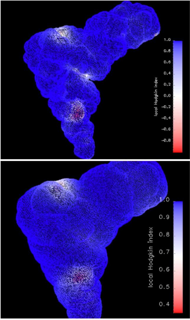
Local Hodgkin Index values obtained from the comparison of the electrostatic potential surface maps between t and t9 systems (see Table I) calculated using the n2 ionic strength scheme (see Table III). The index value is mapped onto the ion accessible surface (top figure) and a surface 6 Å beyond (bottom figure).

3.2 Comparison of nonlinear and linear PB calculations and ionic conditions

This section describes the differences in the potentials obtained for the same tRNA system but derived with different forms of the PB equation or mobile ion compositions (see Table III).

Comparisons of the potential surface maps between calculations l2/n2 and n1/n2 are presented in Figure 6, respectively. We find that the water molecules coordinating metal ions do not significantly change the differences between compared pairs of potentials - the points for t6w, t6wb and t9w systems coincide with corresponding points for t6, t6b and t9 systems, hence for clarity they are not presented in Figure 6.

Figure 6.

Hodgkin Index between: a) l2 and n2 calculations (see Table III). Indices were obtained from the comparison of electrostatic potential surface maps for various tRNA systems (for description see Table I); b) n1 and n2 calculations (see Table III). Comparisons are shown for electrostatic potential surface maps of t, t6, t6b, and t9 (see Table I). Data are presented as a function of the distance from the tRNA surface.

Comparisons of surface potentials between l2 and n2 show sensitivity to the net charge of the system (HI is presented in Figure 6a). RMSD confirms this observation and shows a monotonic decrease from ≈ 6 kT/e at a vdW surface to ≈ 0.2 kT/e 10Å beyond the tRNA surface (data not shown). The dependence on the net charge of tRNA is also distinguished in the free energy differences (defined below eq. 16) between calculations with different PB equations and ionic strengths presented in Figure 7.

Figure 7.

The differences in the electrostatic free energy, ΔG_n2n1 = G_n2 - G_n1, ΔG_l2l1 = G_l2 - G_l1 for various tRNA systems (see Table I).

By examining the similarity indices obtained from calculations with different ionic conditions, n1/n2, we obtain contradictory results. HI in Figure 6b decreases with distance from the tRNA surface meaning that the compared sets loose similarity. On the other hand, RMSD decreases with distance as well showing an increasing similarity of the compared sets (data not shown). Such an opposite result might be explained by the definition of the indices. HI is a measure of proportional difference, while RMSD is a measure of an absolute difference (regardless of the absolute values in the compared sets). Although ionic strength does not change the potentials significantly, it systematically changes the overall distribution of mobile ions. This change is captured by HI (Figure 6b). The behavior is confirmed in Figure 8, which gives no clear regions of difference at a distance of 6 Å away from the tRNA surface. Local HI is almost uniformly distributed with a mean value close to 0.9.

Figure 8.

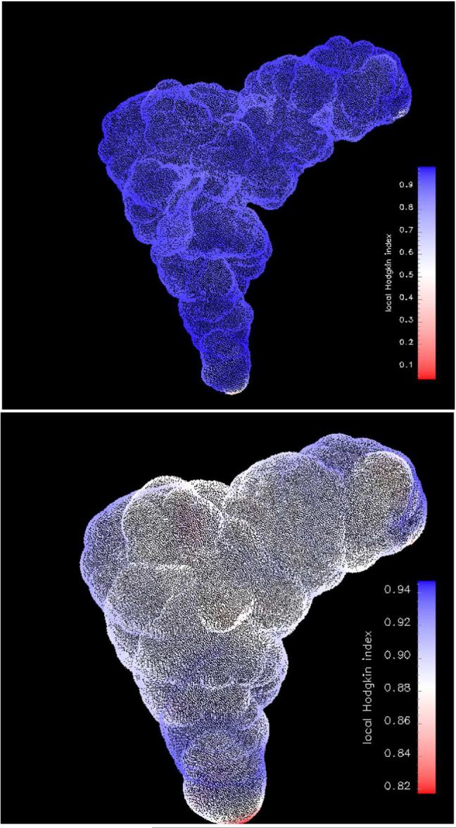
Local Hodgkin Index between n1 and n2 (see Table III) calculations for t system (see Table I). The index values are shown on the ion accessible surface (top figure) and on a surface 6 Å beyond the molecular surface (bottom figure).

The above considerations render HI the most useful of the indices (together with Tanimoto index which has quite similar definition to HI) because it can capture the overall difference between the compared sets.

3.3 Ionic concentration cutoff

To calculate the excess numbers of ions in accord with Eqs. (9) and (10), we used the distribution of Na⁺ ions around bare tRNA obtained from the conventional nonlinear PB model (t system with the n1 salt conditions, see Table III). The calculations were performed for various values of a, namely 1, 2.4 and 3.8 Å. The first one corresponds to the Pauling radius of a bare Na⁺ ion [40]. The second a value is the effective cavity radius of Na⁺ [41] which is equivalent to Pauling radius increased by the radius of a water molecule. The third a is the ion/solvent exclusion radius of a solvated Na⁺ ion, which is equivalent to the Pauling radius increased by the diameter of a water molecule. The resulting excess numbers of Na⁺ ions are shown in Table IV. For a < 3.8 Å we have $\Delta \stackrel{‒}{n}=0$ which means that inequality (7) was not violated in any region of space. In this case, the concentration cutoff is unnecessary. For a equal to 3.8Å, inequality (7) indicates an excess amount of 4.7 ions which can be reproduced with the concentration cutoff scaled with a factor α equal to 4. This factor yields an effective cutoff of $c_i^{\mathit{max}}=4\times 7.2M\simeq 29\mathrm{M}$.

Table IV.

Excess number of ions (Na⁺ or/and Mg²⁺) next to tRNA in the nonlinear PB model according to di erent criteria for the maximum concentration (Eqs. 9 and 10). a is ionic radius, α is a parameter which scales the cuto c_max (Eq. 8). n1 and n2 as in Table III.

	aNa [Å]	aMg [Å]	$\Delta \stackrel{‒}{n}=0$	Δnα=1	Δnα=2	Δnα=3	Δnα=4
n1	1.0	-	0	0.1	0	0	0
	2.4	-	0	4.6	2.0	1.1	0.7
	3.8	-	4.7	12.9	8.2	6.0	4.6
n2	3.8	-	0	0	0	0	0
	-	3.5	0	4.3	2.6	1.9	1.4
	3.5	3.5	0	6.0	4.2	2.4	1.8

The concentration cutoff with a properly calibrated value of $c_i^{\mathit{max}}$ allows to reproduce condition (7) both in terms of the overall number of excess ions and the spatial distribution of the excess concentration. Figure 9 presents excess distribution of Na⁺ ions next to a molecular surface of t system according to condition (7) (left image) and according to a simple cutoff condition with the scaling factor α = 4 (right image).

Figure 9.

Ion accessible surface of the t system from the n1 calculations. Left image: Grid points contributing to the excess number of ions $\Delta \stackrel{‒}{n}=4.7$ (eq. 10). Right image: grid points contributing to the excess number of ions Δn^α = 4.6 (eq. 9) with α = 4.

The excess numbers of ions for distributions of Na⁺ and Mg²⁺ ions resulting from the nonlinear PB model for the t system with the n2 salt conditions (Table III) was also calculated. Table IV shows the excess numbers calculated indepedently for two ionic species, using the radii of solvated ions, 3.8 Å fordglin Na⁺, and 3.5 Å for Mg²⁺. We also estimated the overall excess number of ions of both types from the sum of the two distributions and assuming a common radius of 3.5 Å for both species. Results show that neither the concentrations of the individual species nor the sum of concentrations are violating the inequality (7). We conclude that divalent and slightly smaller Mg²⁺ ions supersede monovalent Na⁺ ions, so as the total concentration of ions of both types next to the molecular surface is lower than concentration of Na⁺ in case of an Mg²⁺-free solution.

Using the modified PB model described in section 2.3 we studied the influence of the ionic concentration cutoff on the electrostatic potential of tRNA and also on electrostatic free energy differences between tRNA systems surrounded by various ionic conditions. First, we compare the HI values for electrostatic potentials obtained from the conventional PB model, and from the modified PB model with a cutoff c^max for Na⁺ ions equal to 20 and 30 M (the corresponding cutoff values for Mg²⁺ ions are 80 and 120 M). Results are presented in Figure 10a which shows that in case of n1 scheme (i.e., only Na⁺ ions) the concentration cutoff affects the potential at short range - up to 4 Å from the molecular surface. Results of the n2 ionic strength scheme (both Na⁺ and Mg²⁺) are only slightly a ected. One should note though, that in the case of n2 calculations, the concentration cutoff applied to Mg²⁺ ions was artificially high, namely it corresponded to the Mg²⁺ concentration cutoff 4 times larger than that of Na⁺.

Figure 10.

Hodgkin Index between calculations: a) with and without ionic concentration cutoff for the t system (see Table I) at various salt conditions; b) n1 and n2, both with ionic concentration cutoff. Data are presented as a function of the distance from the tRNA surface. The c^max values (20M and 30M) provided in the legend refer to Na⁺ concentration and correspond to 80M and to 120M of Mg²⁺ concentration, respectively.

In Figure 10b we show the HI for potentials obtained with the concentration cutoffs (20 and 30 M) for different ionic conditions (see Table III). This figure can be compared with Figure 6b because the latter presents corresponding results obtained from calculations without the concentration cutoff. As shown in Figure 10, at a distance 4 Å beyond the molecular surface the differences in the potentials are not really affected by the concentration cutoff. This arises because the concentration cutoff applies only to regions with absolute high potentials and such regions are located close to the tRNA surface. The effect of concentration cutoff is pronounced more strongly for highly charged systems (compare t and t9w in Figure 10b).

The energetic effect of the concentration cutoff, Eq. (14), is presented in Figure 11 (top). These calculations were performed with concentration cutoffs of Eq. (8) and with the α parameter in the range from 3 to 500. Based on previous results, we note that a physically meaningful value is α ≃ 4, or equivalently $c_{\mathrm{Na}}^{\mathit{max}}\simeq 30$ ≃ 30. The concentration cutoff influences more strongly calculations with the n1 (only Na⁺) ionic strength scheme than those with the n2 (Na⁺ and Mg²⁺) scheme (Tables I and II). As already mentioned, the introduction of divalent cations eliminates the problem of excess ions. The maximum concentration for Mg²⁺ ions is larger than the maximum concentration for Na⁺ ions, thus more Mg²⁺ ions can be packed at regions with high electrostatic potential and, hence, one obtains stronger short-length screening of the tRNA charge. This effect is weaker for the t9w system, in which explicit ions are present, reducing the net charge of the system. The plot in the bottom part of Figure 11 presents ΔΔG values for t and t9w tRNA systems. It shows that the concentration cutoff above 200 M does not strongly affect the results.

Figure 11.

Top plot: the electrostatic free energy difference ΔG due to the cutoff (see eq. 14). Bottom plot: ΔΔG as defined by eq. 15. Data are presented as a function of the Na⁺ concentration cutoff (maximal concentrations of Mg²⁺ and Cl^- ions are varied correspondingly, see text).

We also analyzed the terms contributing to the total ΔΔG, i.e. ΔΔG^fix, ΔΔG^diel, and ΔΔG^mob (see description following Eq. 2). These results showed qualitatively similar behaviour as total ΔΔGs in Figure 11, which confirmed that the concentration cutoff affects all of the contributing terms, even though it is applied only to ΔG^mob term.

The free energy change of the linearization given by Eq. 5, was also calculated. We obtained approximately 376 and 424 kJ/mol for the t system with ionic strengths 0.15 and 0.21 M, respectively (Table III). For t9w system the corresponding results were 151 and 182 kJ/mol for lower and higher ionic strengths, respectively. Again, the less charged the studied system, the smaller the difference between the linear and nonlinear results.

HI values between the potential surface maps obtained from the linear PB equation and a nonlinear one with a concentration cutoff, were calculated as a function of distance from the molecular surface. Results are presented in Figure 12 for two values of the ionic concentration cutoff applied for the mobile Na⁺ and Cl^- ions. The cutoff has only a slight influence on the similarity index. In case of analogous calculations but with additional Mg²⁺ mobile ions, we found that the resulting HIs give no difference to corresponding results obtained without the concentration cutoff of Figure 6a. This remains in agreement with previous conclusions that Mg²⁺ ions replace monovalent Na⁺ ions in the vicinity of the tRNA and suppress the effect of ionic concentration cutoff.

Figure 12.

Hodgkin Index between the l1 calculation without ionic concentration cutoff and the n1 calculation with ionic concentration cutoff. c^max labels are defined as in Figure 10.

To test the dependence of the electrostatic free energies given by Eqs 14 - 16 on the grid resolution, a set of calculations with a different grid spacing (0.3 Å instead of the standard 0.4 Å) was performed. The results were qualitatively similar to those presented in Figure 11.

4 Conclusions

Within the framework of the PB model, we investigated the electrostatic potential around the tRNA molecule, together with the influence of the ionic concentration cutoff on both the electrostatic potential and the electrostatic free energy differences. Electrostatic potentials were generated for different tRNA systems with different number of explicit bound ions and at various physiologic ionic strengths. We verified the applicability of several similarity indices - RMSD, residual function and Hodgkin index.

Not surprisingly, we found that fisrt of all the electrostatic potential depends on the total charge of the tRNA molecule. Moreover, a small change in the fixed charge distribution modifies the potential only locally, in proximity of the site of this change, so global similarity indices can hardly detect this and one needs to use local similarity indices. Changing the ionic strength changes the overall distribution of mobile ions which is captured both by HI and RF. Calculations also showed that the crystallographic water molecules can be removed without a significant change in the electrostatics around tRNA. Surface maps of local HI allowed to determine the regions of large differences in electrostatic potentials. For the compared tRNA systems, the differences are located at the structurally different regions, namely crystallographic ion sites. However, the range of these differences is not identical, showing the importance of all three Mn²⁺ ions, particularly mn1 (see Figure 1). Additionally, surface maps of local similarity indices confirmed the overall change in the distribution of mobile ions when changing the ionic conditions. With regard to global similarity indices ionic conditions, in the studied range, turned out not to be significant.

The similarity indices distinguish the forms of the PB equation (linear and nonlinear) even though the qualitative results obtained with HI and RF are rather contradictory (Figure 2). Other comparisons show that the electrostatic free energy change of adding divalent mobile ions is smaller in the case of the linear PB equation (Figure 3). The difference between the results obtained with the linear and nonlinear PB equations, measured with distance dependent similarity indices, shows sensitivity to the net charge of the system (Figure 6a).

To account for the fact that mobile ions around the solute are of finite size, we applied an ionic concentration cutoff to the electrostatic potential in the Boltzmann distribution. We showed that the cutoff is not important for bare ions but it is necessary if one assumes that ions approach each other through their solvation shells. In this case the Na⁺ concentration cutoff of around 30 M applied to the solution of the nonlinear PB equation reproduces the effect of the exact condition for the maximum concentration represented with inequality (7). When the ionic concentration cutoff is implemented self-consistently to the PB equation it changes each of the contributing parts of the global electrostatic free energy, as well as the electrostatic potential at a distance closer than 4Å from the surface of the tRNA. The cutoff effects are substantial in case of NaCl solution but are supressed upon adding small amount of MgCl₂ because the strongly charged and smaller divalent Mg²⁺ ions supersede the monovalent Na⁺ ions next to the molecular surface.

In monovalent salt and in the region up to 4Å from the tRNA surface where the cutoff is meaningful, the results obtained with a concentration cutoff resemble more the ones obtained with a linear PB equation than those obtained with a nonlinear one. The free energy change resulting from introducing the concentration cutoff in the nonlinear PB equation (Eq. 14) is not negligible only in the case of monovalent salt and for a 20-30 M cutoff (Figure 11). The free energy change resulting from linearization of the PB equation (as given in Eq. 5 is an order of magnitude higher.

These studies will form the basis for the application of the PB model to other highly charged biomolecules but of much larger size.

References

- [1].Gilson MK, Sharp KA, Honig BH. J. Comput. Chem. 1988;9:327–335. [Google Scholar]
- [2].Zhou H. J. Chem. Phys. 1994;100:3152–3162. [Google Scholar]
- [3].Baker NA, McCammon JA. In: Structural Bioinformatics. Weissig H, Bourne PE, editors. John Wiley & Sons; New York: 2003. pp. 427–440. [Google Scholar]
- [4].Baker NA. Methods in Enzymology. Vol. 383. Academic Press; San Diego, CA: 2004. pp. 94–118. [DOI] [PubMed] [Google Scholar]
- [5].Sharp KA, Honig B. J. Phys. Chem. 1990;94:7684–7692. [Google Scholar]
- [6].Sharp KA, Honig B. Ann. Rev. Biophys. Chem. 1990;19:301–332. doi: 10.1146/annurev.bb.19.060190.001505. [DOI] [PubMed] [Google Scholar]
- [7].Ray J, Manning GS. Langmuir. 1994;10:2450–2461. [Google Scholar]
- [8].Odijk T. Macromolecules. 1994;27:4998–5003. [Google Scholar]
- [9].Koculi E, Hyeon C, Thirumalai D, Woodson SA. J. Am. Chem. Soc. 2007;129:2676–2682. doi: 10.1021/ja068027r. [DOI] [PMC free article] [PubMed] [Google Scholar]
- [10].Ma C, Baker NA, Joseph S, McCammon JA. J. Am. Chem. Soc. 2002;124:1438–1442. doi: 10.1021/ja016830+. [DOI] [PubMed] [Google Scholar]
- [11].Trylska J, McCammon JA. J. Am. Chem. Soc. 2005;127:11125–11133. doi: 10.1021/ja052639e. III, C. L. B. [DOI] [PubMed] [Google Scholar]
- [12].Yang G, Trylska J, Tor Y, McCammon JA. J. Med. Chem. 2006;49:5478–5490. doi: 10.1021/jm060288o. [DOI] [PubMed] [Google Scholar]
- [13].Borukhov I, Andelman D, Orland H. Phys. Rev. Lett. 1997;79:435–438. [Google Scholar]
- [14].Borukhov I, Andelman D, Orland H. Electrochimica Acta. 2000;46:221–229. [Google Scholar]
- [15].Chu VB, Bai Y, Lipfert J, Herschlag D, Doniach S. Prepublished - Biophys. J. 2007 doi: 10.1529/biophysj.106.099168. [DOI] [PMC free article] [PubMed] [Google Scholar]
- [16].Kirkwood JG. J. Chem. Phys. 1934;2:767–781. [Google Scholar]
- [17].Levine S, Bell GM. J. Phys. Chem. 1960;64:1188–1195. [Google Scholar]
- [18].Outhwaite CW. Mol. Phys. 1974;27:561–575. [Google Scholar]
- [19].Levine S, Outhwaite CW. J. Chem. Soc., Faraday Trans. 1978;74:1670–1689. [Google Scholar]
- [20].Carnie SL, Torre GM. In: Advances in Chemical Physics. Prigogine I, Rice SA, editors. Vol. 56. John Wiley and Sons; 1984. pp. 141–253. [Google Scholar]
- [21].Vlachy V. Annu. Rev. Phys. Chem. 1999;50:145–165. doi: 10.1146/annurev.physchem.50.1.145. [DOI] [PubMed] [Google Scholar]
- [22].Gavryushov S, Zielenkiewicz P. Biophys. J. 1998;75:2732–2742. doi: 10.1016/S0006-3495(98)77717-3. [DOI] [PMC free article] [PubMed] [Google Scholar]
- [23].Zhi-Jie Tan, Shi-Jie Chen. J. Chem. Phys. 2005;122:044903. [Google Scholar]
- [24].Chin K, Sharp KA, Honig B, Pyle AM. Nat. Struct. Biol. 1999;6:1055–1061. doi: 10.1038/14940. [DOI] [PubMed] [Google Scholar]
- [25].Misra VK, Draper DE. J. Mol. Biol. 2000;299:813–825. doi: 10.1006/jmbi.2000.3769. [DOI] [PubMed] [Google Scholar]
- [26].Polozov RV, Montrel M, Ivanov VV, Melnikov Y, Sivozhelezov VS. Biochemistry. 2006;45:4481–4490. doi: 10.1021/bi0516733. [DOI] [PubMed] [Google Scholar]
- [27].Shi H, Moore PB. RNA. 2000;6:1091–1105. doi: 10.1017/s1355838200000364. [DOI] [PMC free article] [PubMed] [Google Scholar]
- [28].Carbo RL, Arnau M. Int.J.Quantum Chem. 1980;17:1185–1189. [Google Scholar]
- [29].Hodgkin EE, Richards WG. Quantum Biol.Symp. 1987;14:105–110. [Google Scholar]
- [30].Misra VK, Draper DE. Biopolymers (Nucleic Acid Sciences) 1998;48:113–135. doi: 10.1002/(SICI)1097-0282(1998)48:2<113::AID-BIP3>3.0.CO;2-Y. [DOI] [PubMed] [Google Scholar]
- [31].Baker NA, Sept D, Joseph S, Holst MJ, McCammon JA. Proc. Natl. Acad. Sci. 2001;98:10037–10041. doi: 10.1073/pnas.181342398. [DOI] [PMC free article] [PubMed] [Google Scholar]
- [32].Kilic MS, Bazant MZ, Ajdari A. Phys. Rev. E. 2007;75:021502. doi: 10.1103/PhysRevE.75.021502. [DOI] [PubMed] [Google Scholar]
- [33].Grochowski P, Trylska J. Biopolymers. 2008;89:93–113. doi: 10.1002/bip.20877. [DOI] [PubMed] [Google Scholar]
- [34].Case DA, Darden TA, Cheatham TE, III, Simmerling CL, Wang J, Duke RE, Luo R, Merz KM, Wang B, Pearlman DA, Crowley M, Brozell S, Tsui V, Gohlke H, Mongan J, Hornak V, Cui G, Beroza P, Schafmeister C, Caldwell JW, Ross WS, Kollman PA. AMBER 8. University of California; San Francisco: 2004. [Google Scholar]
- [35].Holst MJ, Saied F. J. Comp. Chem. 1995;16:337–364. [Google Scholar]
- [36].Holst M, Baker N, Wang F. J. Comput. Chem. 2000;21:1319–1342. [Google Scholar]
- [37].Beard DA, Schlick T. Biopolymers. 2001;58:106–115. doi: 10.1002/1097-0282(200101)58:1<106::AID-BIP100>3.0.CO;2-#. [DOI] [PubMed] [Google Scholar]
- [38].M.Downs G, Willett P. In: Reviews in Computational Chemistry. Boyd DB, editor. Vol. 7. Wiley-VCH; New York: 1995. [Google Scholar]
- [39].Wade RC, Gabdoulline RR, de Rienzo F. Int. J. Quant. Chem. 2001;83:122–127. [Google Scholar]
- [40].Pauling L. J. Am. Chem. Soc. 1927;49:765–790. [Google Scholar]
- [41].Marcus Y. J. Sol. Chem. 1983;4:271–275. [Google Scholar]
- [42].Alberts B, Bray D, Lewis J, Roff M, Roberts K, Watson JD. Molecular Biology of the cell. Garland Publishing Inc.; New York and London: 1994. 1983, 1989. [Google Scholar]