Prediction of protein secondary structure by mining structural fragment database

Abstract

A new method for predicting protein secondary structure from amino acid sequence has been developed. The method is based on multiple sequence alignment of the query sequence with all other sequences with known structure from the protein data bank (PDB) by using BLAST. The fragments of the alignments belonging to proteins from the PBD are then used for further analysis. We have studied various schemes of assigning weights for matching segments and calculated normalized scores to predict one of the three secondary structures: α-helix, β-sheet, or coil. We applied several artificial intelligence techniques: decision trees (DT), neural networks (NN) and support vector machines (SVM) to improve the accuracy of predictions and found that SVM gave the best performance. Preliminary data show that combining the fragment mining approach with GOR V (Kloczkowski et al, Proteins 49 (2002) 154–166) for regions of low sequence similarity improves the prediction accuracy.

1. Introduction

One of the ultimate goals of computational biology is reliable prediction of the three-dimensional structure of proteins from sequences because of significant difficulties in obtaining high resolution crystallographic data. An intermediate but useful step is to predict the secondary structure, which might simplify the complicated 3D structure prediction problem. This reduces the difficult 3D structure determination to a simpler one-dimensional problem. This reduction is possible since proteins can form local conformational patterns like α-helices and β-sheets. Many have shown that predicting secondary structure can be a first step toward predicting 3D structure [1–4].

Sometimes, secondary structure prediction can even be useful when a protein native structure is already known, for example to predict amyloid fibrils: misfolded β-sheet-rich structures, responsible for Alzheimer’s and Parkinson’s diseases [5].

Secondary structure prediction can be used to predict some aspects of protein functions; in genome analysis, it is used to help annotate sequences, classify proteins, identify domains, and recognize functional motifs [6].

First attempts at secondary structure prediction were based mainly on single amino acid propensities. In order to improve prediction accuracies, some researchers began including evolutionary information in the prediction procedure [7,8]. These attempts consist of folding evolutionary propensities into the prediction by introducing a measure of sequence variability.

Enlarged databases, new searching models and algorithms make it feasible to extend family divergence, even when the structures of some of the protein family members are unknown (e.g. large-scale searches with PSI-BLAST [9] or Hidden Markov Models [10,11]). By using divergent profiles, the prediction accuracy reached 0.76 in Q₃ (the fraction of correctly predicted residues in one of the three states: helix, strand, and other, see definition in methods). It is believed that enlarged databases and extended searching techniques contributed significantly to the increase in the accuracy of the secondary structure prediction.

There exist several popular and historically important prediction methods, including empirical statistical methods [12], information theory [13–16], nearest neighbor [17], hidden Markov models [18], and artificial intelligence (AI) approaches [19].

As one of the AI approaches, neural networks simulate the operations of synaptic connections among neurons. As the neurons are layered to process different levels of signals, the neural networks accept the original input (which might be a sequence segment, having been modified by a weighting factor), combine more information, integrate all to an output, send the output to the next level of processor, and so on. During this process, the network adjusts the weights and biases continuously, according to the known information, i.e. the network is trained on a set of homologous sequences of known structures for the secondary structure prediction problem. The more layers it has, the more information it distinguishes. The PHD [19] is one representative method, with the most recent versions reporting accuracy of prediction up to 0.77.

In the field of ab initio protein structure prediction, the Rosetta algorithm, a computational technique developed by Baker and his colleagues at the University of Washington, was quite successful in predicting the three-dimensional structure of a folded protein from its linear sequence of amino acids during the fourth (2000) and the fifth (2002) Critical Assessment of Techniques for Protein Structure Prediction (CASP4, CASP5), and most recently during CASP6 (2004).

Based upon the assumption that the distribution of structures sampled by an isolated chain segment can be approximated by the distribution of conformations of that sequence segment in known structures, Rosetta predicts local structures by searching all possible conformations. The popular view is that folding to the native structure occurs when conformations and relative orientations of the segments allow burial of the hydrophobic residues and pairing of β-strands without steric clashes [20].

It is commonly believed that similarities between the sequences of two proteins infer similarities between their structures, especially when the sequence identity is greater than about 25%. Most protein sequence folds into a unique three-dimensional structure, yet sometimes highly dissimilar sequences can assume similar structures. From an evolutionary point of view, the structure can be more conserved than sequence.

The sequence similarity of very distant homologues is difficult to identify. But the conservation of some special motifs can possibly be captured using special methods. Those special motifs are more important than general matches found in alignments of close homologues due to their uniqueness. The problem of such detection is usually confounded by the use of structure-independent sequence substitution matrices.

Since a similar sequence implies a similar structure and conserved local motifs may assume a similar shape, we attempt to find a local alignment method to obtain structure information to predict the secondary structure of query sequences. For this study, we assembled a set of segments obtained through local sequence alignment and use this information for predictions. We applied BLAST on query sequences against a structure database in which all the information of proteins is available (PDB or DSSP), and then use these results to introduce evolutionary information into predictions. We applied various weighting procedures to the matches based on the sequence similarity scores. Finally, we calculated the normalized scores for each position and for each secondary structure at that position. Note that since the scores of being E, H or C are sometimes close or even equal, so that choosing the highest score is either not possible or not fully justifiable. Furthermore, the predicted secondary structure element is not physically meaningful in all cases, such as helices having only two residues, or mixtures of strand (E) and helix (H) residues. Therefore, instead of predicting the secondary structure with the highest score, we incorporated artificial intelligence (AI) approaches for the final secondary structure assignment.

2. Methods

In the prediction and evaluation part, for each query sequence from the dataset, we assign weights to the matching segments obtained from BLAST, calculate normalized scores for each residue, predict the secondary structure for that residue according to the normalized scores, and finally, calculate Q₃ (an accuracy measure [16]) and Matthews’ correlation coefficients [21]. In the weight assignment part, several parameters are considered, including different substitution matrices, similarity/identity cutoffs, degree of exposure of residues to solvent, and protein classification and sizes. Two strategies are applied to predict the secondary structure according to the normalized scores of residues. One method is to choose the highest-score structure class as the prediction, and the other is to use AI (artificial intelligence) approaches to choose a classification based on training.

Fig. 1 shows the flowchart of our approach.

Fig. 1.

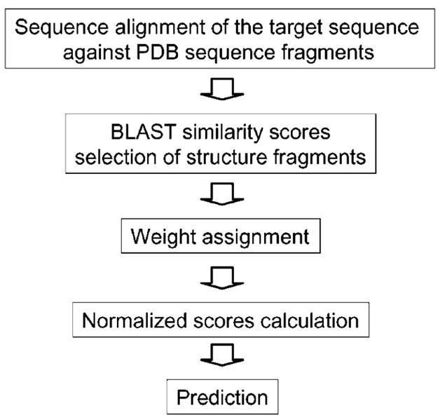
The secondary structure prediction scheme.

The 513 non-redundant domains collected by Cuff and Barton [22,23] have been selected as the query test sequences (CB513). Local sequence alignment using BLAST has been applied with blastcl3 on CB513 sequences using different parameters. We use different substitution matrices, including BLOSUM-45, -62, and -80, PAM-30 and -70.

2.1. Secondary structure elements interpretation

We follow a three-state identification of secondary structures, namely, helix (H), extended (β-sheet) (E), and coil (C). Because it provides a consistent set of secondary structure assignments, we have utilized a reduced version of DSSP [24] (Database of Secondary Structure in Proteins) classification that uses eight types of secondary structure assignment: H (α-helix), E (extended β-strand), G (3₁₀ helix), I (π-helix), B (bridge, a single residue β-strand), T (β-turn), S (bend), and C (coil). For our translation, we follow the strategy of CASP [25] (Critical Assessment of Techniques for Protein Structure Prediction), and reduce the DSSP alphabet in the following manner: helices (H, G, and I) in the DSSP code are assigned the letter H in the three-letter secondary structure code; whereas strands (E) and bridges (B) in the DSSP code are translated into sheets (E). Other elements of the DSSP structure (T, S, C) are translated into coil (C).

2.2. Weight assignment for matches of segments

We define identity scores and their powers (id^c, where c is a positive real number) as the weights of matching segments. Here id is a fraction, representing the ratio of the number of exact matches of residues to the total number of residues in the matching segment. Weights are adjusted when different parameters are considered. This procedure will be illustrated in the parameter section.

2.3. Calculation of normalized scores for each residue

The prediction is position-based (residue by residue for the query sequences). At each position, the predicted secondary structure is determined by the actual secondary structures of segments matching at that position. Each match is assigned a weight according to the similarity or identity score of the alignment from BLAST. At each position, the weights are normalized, and the normalized scores for the position being in each of secondary structure states are calculated. Our procedure of normalized score calculation is illustrated in the following example (Fig. 2).

Fig. 2.

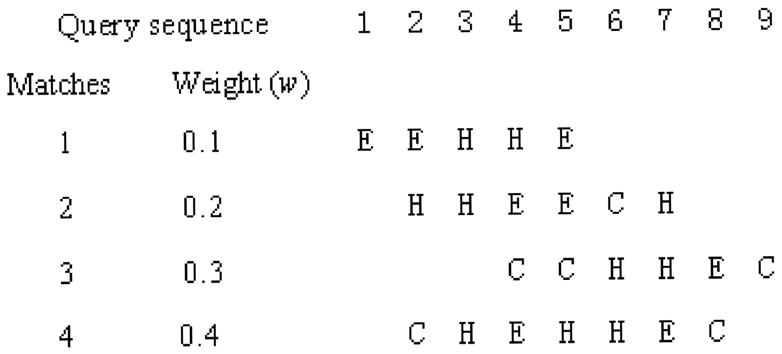
An example showing a query sequence and its matching segments (sequences not shown). The query sequence residues are represented with their sequence position numbers. The matching segments are expressed as secondary structure elements. The weights are shown for each segment.

Define s(H, i) as the normalized score for position i to be in the state H.

$$s(\text{H},i)=\frac{\sum w(\text{H},i)}{\sum w(\text{H},i)+\sum w(\text{E},i)+\sum w(\text{C},i)}$$ (1)

where w(H, i) is the weight for one matching segment with residue at the ith position in a helix. w(E, i) and w(C, i) are similarly defined.

For the example above, if we show few cases:

$$\begin{array}{l}s(\text{H},2)=0.2/(0.1+0.2+0.4)\\ s(\text{H},4)=0.1/(0.1+0.2+0.3+0.4)\\ s(\text{E},4)=(0.2+0.4)/(0.1+0.2+0.3+0.4)\end{array}$$ (2)

2.4. Parameters adjusted for weight assignments

We have used two different types of substitution matrices: PAM and BLOSUM. PAM (Percent Accepted Mutation) matrix was introduced by Dayhoff [26] to quantify the amount of evolutionary change in a protein sequence, i.e. how often different amino acids replace other amino acids in evolution based on a database of 1572 changes in 71 groups of closely related proteins. BLOSUM (Blocks Substitution Matrix) was introduced by Henikoff [27] to obtain a better measure of differences between two proteins, specifically for distantly related proteins. It is a substitution matrix in which scores for each position are derived from observations of the frequencies of substitutions in blocks of local alignments in related proteins. The blocks were constructed by PROTOMAT from 504 non-redundant groups of proteins catalogued in Prosite 8.0 [28] keyed to Swiss-Prot. We also have used BLOSUM-45, -62, -80 and PAM-30, -70 in BLAST alignments in our calculations.

Because we are testing the concept of fragment assembly for secondary structure prediction, we choose to limit the extent of similarity or identity to be included. Different cutoffs of similarity or identity scores of matches are set. Cutoffs include 99, 90, 80, 70, and 60%. The matches with similarity or identity scores higher than a cut-off are eliminated from matching lists of segments, which are used to calculate normalized scores of residues.

In order to include approximate tertiary information in the secondary structure calculations, we calculated the degree of exposure to solvent for residues in the 13,432 sequences in PDB (out of 21,754 sequences available by 7/21/2003). Naccess software (http://wolf.bms.umist.ac.uk/naccess/) has been used to calculate the solvent accessibility of residues for each protein in this data set. A residue indexed file is thus constructed that includes the solvent accessibility status of each residue. This residue file is used to differentiate buried and exposed residues by assigning different weights. If the relative accessibility of a residue is less than 5.0, it is regarded as a buried residue; if the relative accessibility of a residue is greater than 40.0, it is regarded as an exposed residue; the rest are regarded as intermediate residues. Buried residues are weighted more heavily.

2.4. Prediction based on normalized scores of residues

The secondary structure element having the highest score is chosen as the final predicted result for a given residue. For a specific position of a query sequence, we have three normalized scores for the residue for each secondary structure state (s(H, i), s(E, i), and s(C, i)). In this prediction scheme, we always choose the highest score among these three scores to determine the prediction for that residue.

We also apply AI techniques to modify the final secondary structure in the decision step. Instead of assigning the secondary structure for a specific position according to the highest normalized score of the secondary structure at that position, we applied artificial intelligence approaches to choose the most appropriate normalized score according to learning results from training sets. We used decision trees (DT), neural networks (NN), and support vector machines (SVM) and compared their predictions. The main idea of these AI approaches is to gather information from a training set and use it to predict for a new test set. In our case, the ratio of the number of training and test sequences is 4:1. We first formed a file that contains all the normalized scores for all the query sequences from the benchmark dataset, then randomly partitioned these scores into training and test sets, and finally applied AI approaches for the prediction.

2.5. Measures for prediction evaluation

The most common parameter used to measure prediction accuracy is Q₃, which is the fraction of all correctly predicted residues within the three state (H, E, C) classes. An accuracy matrix [A_ij] of size 3×3 (i and j stand for the three states H, E, C) is introduced. The ij-th element A_ij of the accuracy matrix is the number of residues predicted to be in state j, which, according to the PDB data, is actually in state i. Obviously, the diagonal entries of [A_ij] represent the number of correctly predicted residues. Q₃ is therefore, defined as:

$$Q_3=\frac{{\sum }_{i=1}^3{A}_{ii}}{N}$$ (3)

where N is the total number of residues in the query sequence, and defined as the total number of all entries of [A_ij]:

$$N=\sum _{i=1}^3\sum _{j=1}^3{A}_{ij}$$ (4)

Another measure of accuracy of prediction that we calculate is Matthews correlation coefficient for helix (C_α), strand (C_β) and coil (C_c) states.

Matthews correlation coefficient for the helix state (C_α) is defined as:

$$C_{\alpha }=\frac{{\text{TP}}_{\alpha }{\text{TN}}_{\alpha }-{\text{FN}}_{\alpha }{\text{FP}}_{\alpha }}{\sqrt{([{\text{TN}}_{\alpha }+{\text{FN}}_{\alpha }][{\text{TN}}_{\alpha }+{\text{FP}}_{\alpha }][{\text{TP}}_{\alpha }+{\text{FN}}_{\alpha }][{\text{TP}}_{\alpha }+{\text{FP}}_{\alpha }])}}$$ (5)

where TP, TN, FN, and FP are the numbers of true positives, true negatives, false negatives, and false positives, respectively.

3. Results and discussion

3.1. Basic method—the weights of matches are defined to be the powers of identity scores of matches

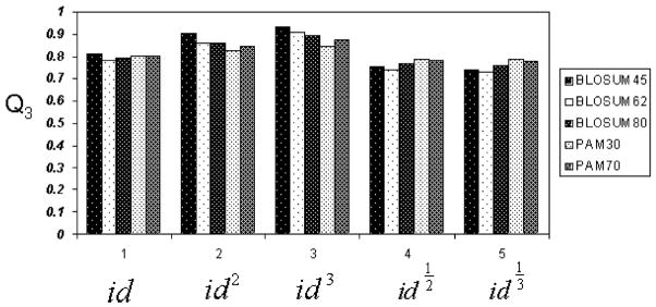
We tried different combinations of matrices and identity powers. The best result comes from using BLOSUM 45 and id³ as the weight assignment method. Fig. 3 shows the basic average prediction accuracies (Q₃) using the different substitution matrices.

Fig. 3.

Basic CB513 prediction accuracy, with bars from left to right designating BLOSUM45, BLOSUM62, BLOSUM80, PAM30, and PAM70 substitution matrices.

3.2. Different identity score cut-offs

3.2.1. All ‘good’ matches are filtered out

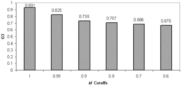
In the following calculations, we use the basic prediction method, and observe the influence of matches at various identity levels by using several identity cut-offs. If the identity score of a match is greater than the cut-off, the match is eliminated from consideration. In this part, we focus mainly on predictions using BLOSUM 45, since it gives better results at different identity cut-off levels. Note that when we use BLOSUM 45 at cut-off levels 0.99 and 0.90, the Q₃ values become 0.825 and 0.735, respectively.

Fig. 4 summarizes the tendency of changes with the drops of cut-offs.

Fig. 4.

Prediction accuracies under different identity cut-offs for weights of id³ and BLOSUM 45 substitution matrix.

3.2.2. Perfect matches filtered out, but most strong reasonable matches kept

Matches with the highest identity scores (greater than id cut-off) are filtered out, but the ‘reasonable’ high-id matches are kept. We define the ‘reasonable’ high-id matches to be those matches that have relatively high identity scores (greater than id cut-off), but are not too short (>5 residues), and are not as long as the query sequence (less than 90 or 95% the length of the query sequence).

The prediction accuracy Q₃’s are compared in the following three cases. All results are obtained using BLOSUM45 with id cut-off set to 0.90.

In case 1, all high-id matches (matches with identity scores higher than identity cut-off) are filtered out. This case is used as a control. In case 2, sequences with identity scores greater than id cut-off (0.90 here), lengths longer than five residues, and lengths less than 90% of query sequence are kept. In case 3, sequences with identity scores greater than 90%, lengths longer than five residues, and lengths below 95% of the query sequence are kept. Table 1 gives the accuracies for the above three cases. We observe that id³ gives the highest accuracy in each case.

Table 1.

Prediction accuracies under identity cut-off 90 in three cases

Matrix	id Cut-off	High id matches processing	id1/3	id1/2	id	id2	id3
BLOSUM45	0.90	Case 1 (all filtered)	0.675	0.680	0.697	0.725	0.735
		Case 2	0.677	0.683	0.701	0.730	0.740
		Case 3	0.678	0.683	0.702	0.731	0.742

3.2.3. Effect of exposure of residues to solvent

Here, we show the results when the weights of matches are defined as id³, id cut-off is set to be 0.99, and the BLOSUM 45 matrix is applied. Accordingly, we make the following linear changes to the weights of residues: if a residue is buried, its weight is multiplied by an integer (2); if it is intermediate, we multiply the original weight by 1.5; if exposed, the weight is one. Table 2 gives the Q₃ results. As can be seen, the differentiation of buried and exposed residues does not have a substantial effect on Q₃.

Table 2.

Prediction accuracies (Q₃) with accessibility of residues considered. wt stands for weight, SA for solvent accessibility

Residue status definition	Q3
Control (status not applied)	0.825
wt=2 if SA≤5	0.828
wt=2 if SA≤20	0.829

3.2.4. Accuracies for proteins of different sizes

For these calculations, the dataset is divided into four groups according to sequence sizes: tiny (n≤100 residues, 154 sequences), small (100<n≤200 residues, 216 sequences), large (200<n≤300 residues, 84 sequences), and giant (n>300 residues, 58 sequences). We only considered the case of the BLOSUM 45 matrix, with weight function id³. No optimization was applied. Table 3 shows the prediction accuracies for proteins of different sizes. The accuracies vary from 0.911 for the ‘tiny’ group to 0.948 for the ‘large’ group. Relatively little change is observed across those different categories.

Table 3.

The accuracies of predictions for proteins of different lengths

Groups	CB513	Tiny	Small	Large	Giant
Q3	0.931	0.911	0.936	0.948	0.940

3.2.5. Application of artificial intelligence (AI) approaches

We use AI approaches to determine the final secondary structure prediction based on the normalized scores of some secondary structure elements. The prediction accuracies are measured using Q₃. We consider some popular AI approaches, including decision trees (DT), neural networks (NN), and support vector machines (SVM).

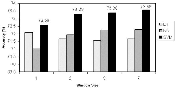
In these calculations, the substitution matrix BLOSUM 45 is used. All matches which are better than 90% are discarded. We randomly partitioned the query dataset into training and testing sets at a ratio of 4:1. Previously, when manually assigning a secondary structure state to a residue according to the highest normalized score of that residue, we obtain the best result of prediction accuracy of Q₃=0.720 for the test set sequences. Fig. 5 shows a comparison among AI approaches for different window sizes (note that our prediction accuracy using the previous method for the test set is exactly the same 0.720). Little improvement is observed in prediction accuracy among decision trees, neural networks and support vector machines.

Fig. 5.

Normalized score based prediction using AI approaches with different window sizes.

3.2.6. Correlation coefficient (CC) of prediction

We calculate average Matthews correlation coefficient for the helix state (C_α), strand (C_β) and coil (C_c) for our prediction, when BLOSUM 45 is applied, identity cut-off 0.99 is set, and the weight is defined as identity score cubed. Table 4 gives the result of correlation coefficient for (C_α), strand (C_β) and coil (C_c) for the 513 sequences. The results shown are either averaged over the number of sequences (sequence average) or over the number of amino acids (AA average).

Table 4.

Correlation coefficients for α-helix, β-strand and coil

Id cut-off		Cα	Cβ	Cc
0.99	Sequence average	0.682	0.614	0.688
	AA average	0.810	0.780	0.739
0.90	Sequence average	0.549	0.472	0.552
	AA average	0.625	0.589	0.553

3.2.7. The parameters corresponding to the case of the highest prediction accuracy

When the weights are defined as the identity score powers, the best accuracy is 0.931. It is obvious that 0.931 is over-estimated, since in a real application, a new query sequence would not likely have a perfect match in alignment against any database. So we filter out some good matches with identity scores higher than a cut-off. The best prediction accuracy for cut-off 0.99 is 0.825, and for 0.90 is 0.735. If some optimization methods (either separate or combined) are applied, we can expect minor improvements in the accuracies. Actually we have seen such a tendency from these optimization methods. We notice that perfect matches play an important role in the accuracy of the prediction. Even a 0.01 cut-off decrease leads to a sharp drop in the prediction accuracy.

Overall, using AI approaches to determine the final prediction according to previously obtained normalized scores yields slightly better results.

3.2.8. Combination of the present approach with GOR V

The GOR [13] (Garnier–Osguthorpe–Robson) method is one of the earliest methods to predict the secondary structure of proteins based on the amino acid frequencies combined with information theory and Bayesian statistics. In the first version of GOR, a data set of 26 proteins was used to derive singlet statistics. Throughout the years, the method has been enhanced continuously: (1) the size of the database was enlarged to 75 proteins in GOR II [14], (2) doublets, additionally to singlets, were used to derive more meaningful statistics in GOR III [29], (3) the protein data set was increased to 267 proteins in GOR IV [15], and finally (4) evolutionary information was added in GOR V [16] based on a database 513 non-redundant proteins. The GOR V server is publicly available at http://gor.bb.iastate.edu/. With these improvements, the accuracy of the GOR method (Q₃) using full jackknife testing reached 73.5% in its final version.

Since GOR predictions do not use any sequence similarity information, they have a higher chance to perform well for low sequence similarities compared to other prediction methods based on database searches. This advantage provided by GOR is harnessed to increase the accuracy of the fragment mining method in the following manner. First, the fragments are identified according to their sequence similarity to the target sequence. Then, the fragments above a minimum similarity cut-off are selected to predict the protein secondary structure using the fragment mining. Since high sequence similarity suggests similar 3D protein structures, the minimum similarity cut-off is taken as 40%. Above this sequence similarity, the fragment mining method is expected to perform well due to strong sequence-structure correlation.

Since a minimum cut-off is enforced, the fragment mining cannot assign a secondary structure to every residue. Therefore, the rest of the assignments are predicted using GOR V method.

Although biological databases are frequently expanded, the sequence alignments obtained using similarity searches may not always contain a perfect match, but instead have a set of matches with varying sequence similarities. In order to test the accuracy of our combined method at different levels of sequence similarities, we defined a maximum sequence similarity cut-off value above which matches are not included in the fragment mining. Therefore, in our combined method, only fragments with sequence similarities between maximum and minimum similarity cut-off values are used for mining predictions; for the rest of the target sequence, the GOR V method is used.

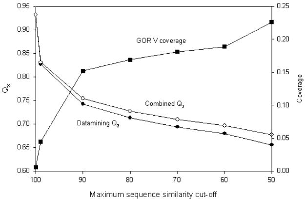
Fig. 6 shows the prediction accuracies for the fragment mining method and the combined method, averaged over 513 proteins. Coverage shows the fraction of target sequence residues predicted by GOR. The minimum sequence similarity is kept constant at 40%. As expected, the fragment mining method performs exceptionally well at high sequence similarities. When the maximum cut-off is reduced to 90%, the fragment mining performs with 74.2% accuracy, which is slightly larger than the average GOR V accuracy of 73.5% for the same protein data set. When combined with GOR V method, the overall accuracy increases by an additional 1.2%. The increase in the overall accuracy is consistently observed for each maximum similarity cut-off value employed in this study. Above 50% maximum cut-off, the fragment mining method scores more than 65% accuracy, and the combined method, more than 67.7%. These results show that combining the fragment mining with GOR can be exploited to increase the secondary structure prediction accuracy for low sequence similarities.

Fig. 6.

Q₃ as a function of sequence similarity cut-off for fragment datamining method, GOR V and the combination of these two methods. The fraction of target sequence residues predicted by GOR in the combined method (coverage) is also shown.

4. Conclusion

The present study shows prediction accuracy comparable to currently popular methods. We find that our method works almost equally well for sequences of different sizes in CB513. Additionally, our method yields comparable prediction accuracies for different folds and secondary structures (all-α, all-β, α + β and α/β) of proteins in the query dataset. The accuracy for all beta sequences is only 1.5% less than for all-α sequences. We use some AI approaches in the last step of our prediction, to determine the final secondary structure element according to the normalized score file, and gain 3–4% improvement in accuracy based on the method of choosing the highest normalized score.

Finally, the accuracy of the prediction can be further improved by combining it with the GOR V method for cases when sequence similarity with fragments from the database is below a certain threshold.

References

- 1.Chen CC, Singh JP, Altman RB. Bioinformatics. 1999;15:53–65. doi: 10.1093/bioinformatics/15.1.53. [DOI] [PubMed] [Google Scholar]
- 2.Eyrich VA, Standley DM, Friesner RA. J Mol Biol. 1999;288(4):725–42. doi: 10.1006/jmbi.1999.2702. [DOI] [PubMed] [Google Scholar]
- 3.Lomize AL, Pogozheva ID, Mosberg HI. Proteins. 1999;(Suppl 3):199–203. doi: 10.1002/(sici)1097-0134(1999)37:3+<199::aid-prot25>3.3.co;2-p. [DOI] [PubMed] [Google Scholar]
- 4.Ortiz AR, Kolinski A, Rotkiewicz P, Ilkowski B, Skolnick J. Proteins. 1999;(Suppl 3):177–85. doi: 10.1002/(sici)1097-0134(1999)37:3+<177::aid-prot22>3.3.co;2-5. [DOI] [PubMed] [Google Scholar]
- 5.Yoon S, Welsh WJ. Protein Sci. 2004;13(8):2149–60. doi: 10.1110/ps.04790604. [DOI] [PMC free article] [PubMed] [Google Scholar]
- 6.Rost B, Eyrich VA. Proteins. 2001;(Suppl 5):192–9. doi: 10.1002/prot.10051. [DOI] [PubMed] [Google Scholar]
- 7.Dickerson RE, Timkovich R, Almassy RJ. J Mol Biol. 1976;100:473–91. doi: 10.1016/s0022-2836(76)80041-1. [DOI] [PubMed] [Google Scholar]
- 8.Zvelebil MJ, Barton GJ, Taylor WR, Sternberg MJ. J Mol Biol. 1987;195(4):957–61. doi: 10.1016/0022-2836(87)90501-8. [DOI] [PubMed] [Google Scholar]
- 9.Altschul SF, Madden TL, Schaffer AA, Zhang JH, Zhang Z, Miller W, et al. Nucl Acids Res. 1997;25(17):3389–402. doi: 10.1093/nar/25.17.3389. [DOI] [PMC free article] [PubMed] [Google Scholar]
- 10.Eddy SR. Bioinformatics. 1998;14:755–63. doi: 10.1093/bioinformatics/14.9.755. [DOI] [PubMed] [Google Scholar]
- 11.Karplus K, Barrett C, Hughey R. Bioinformatics. 1998;14:846–56. doi: 10.1093/bioinformatics/14.10.846. [DOI] [PubMed] [Google Scholar]
- 12.Chou PY, Fasman GD. Biochemistry. 1974;13:222–45. doi: 10.1021/bi00699a002. [DOI] [PubMed] [Google Scholar]
- 13.Garnier J, Osguthorpe DJ, Robson B. J Mol Biol. 1978;120:97–120. doi: 10.1016/0022-2836(78)90297-8. [DOI] [PubMed] [Google Scholar]
- 14.Garnier J, Robson B. The GOR method for predicting secondary structures in proteins. In: Gasman GD, editor. Prediction of protein structure and the principles of protein conformation. New York: Plenum press; 1989. pp. 417–65. [Google Scholar]
- 15.Garnier J, Gilbrat JF, Robson B. Methods Enzymol. 1996;266:540–53. doi: 10.1016/s0076-6879(96)66034-0. [DOI] [PubMed] [Google Scholar]
- 16.Kloczkowski A, Ting KL, Jernigan RL, Garnier J. Proteins. 2002;49(2):154–66. doi: 10.1002/prot.10181. [DOI] [PubMed] [Google Scholar]
- 17.Salamov AA, Solovyev VV. J Mol Biol. 1997;268(1):31–6. doi: 10.1006/jmbi.1997.0958. [DOI] [PubMed] [Google Scholar]
- 18.Bystroff C, Thorsson V, Baker D. J Mol Biol. 2000;301:173–90. doi: 10.1006/jmbi.2000.3837. [DOI] [PubMed] [Google Scholar]
- 19.Rost B, Sander C. Proteins. 1994;19(1):55–72. doi: 10.1002/prot.340190108. [DOI] [PubMed] [Google Scholar]
- 20.Bonneau R, Strauss CEM, Baker D. Proteins. 2001;43:1–11. doi: 10.1002/1097-0134(20010401)43:1<1::aid-prot1012>3.0.co;2-a. [DOI] [PubMed] [Google Scholar]
- 21.Matthews BB. Biochim Biophys Acta. 2004;405:442–51. doi: 10.1016/0005-2795(75)90109-9. [DOI] [PubMed] [Google Scholar]
- 22.Cuff JA, Barton GJ. Proteins. 1999;34(4):508–19. doi: 10.1002/(sici)1097-0134(19990301)34:4<508::aid-prot10>3.0.co;2-4. [DOI] [PubMed] [Google Scholar]
- 23.Cuff JA, Barton GJ. Proteins. 2000;40(3):502–11. doi: 10.1002/1097-0134(20000815)40:3<502::aid-prot170>3.0.co;2-q. [DOI] [PubMed] [Google Scholar]
- 24.Kabsch W, Sander C. Biopolymers. 1983;22:2577–637. doi: 10.1002/bip.360221211. [DOI] [PubMed] [Google Scholar]
- 25.Moult J, Petersen JT, Judson R, Fidelis K. Proteins. 1995;23:II–V. doi: 10.1002/prot.340230303. [DOI] [PubMed] [Google Scholar]
- 26.Dayhoff MO, Schwartz RM, Orcutt BC. Atlas Protein Seq Struct. 1978;(Suppl 3):345–52. [Google Scholar]
- 27.Henikoff S, Henikoff JG. Proc Natl Acad Sci USA. 1992;89:10915–9. doi: 10.1073/pnas.89.22.10915. [DOI] [PMC free article] [PubMed] [Google Scholar]
- 28.Bairoch A. Nucl Acids Res. 1991;25:2241–5. doi: 10.1093/nar/19.suppl.2241. [DOI] [PMC free article] [PubMed] [Google Scholar]
- 29.Gibrat JF, Garnier J, Robson B. J Mol Biol. 1987;198:425–43. doi: 10.1016/0022-2836(87)90292-0. [DOI] [PubMed] [Google Scholar]