Object-oriented Bayesian networks for paternity cases with allelic dependencies

Abstract

This study extends the current use of Bayesian networks by incorporating the effects of allelic dependencies in paternity calculations. The use of object-oriented networks greatly simplify the process of building and interpreting forensic identification models, allowing researchers to solve new, more complex problems. We explore two paternity examples: the most common scenario where DNA evidence is available from the alleged father, the mother and the child; a more complex casewhere DNA is not available from the alleged father, but is available from the alleged father’s brother. Object-oriented networks are built, using HUGIN, for each example which incorporate the effects of allelic dependence caused by evolutionary relatedness.

1. Introduction

Several researchers are using Bayesian networks to aid in the sometimes laborious calculations that are associated with the evaluation of forensic evidence (see [1] for a comprehensive review). The majority of this work makes the assumption that no allelic dependencies are occurring within the population studied. While in the majority of cases this may be a reasonable approximation, there are some cases in which dependencies caused by relatedness have a large impact [2–4]. We show that existing Bayesian networks are easily extended to handle this additional complexity. As a result, more forensic scientists will be able to take into account evolutionary relatedness when evaluating DNA evidence.

1.1. Allelic dependencies and paternity calculations

A body of evidence can be evaluated by calculating a likelihood ratio [5]:

$$\text{LR}=\frac{Pr(E\mid H_{\text{p}})}{Pr(E\mid H_{\text{d}})},$$ (1)

where E denotes the evidence, H_p and H_d denote the plaintiff’s and defendant’s hypotheses, respectively. In paternity cases, the likelihood ratio is termed the paternity index, or PI. Letting PF represent the putative (alleged) father, M the mother, and C the child, one set of hypotheses are

• H_p: PF is the father of C,

• H_d: Some other man is the father of C.

If G_X denotes the genotype of person X, the PI can be simplified (details in [6] Chapter 6) to the ratio of two conditional probabilities:

$$\text{PI}=\frac{Pr(G_{\text{C}}\mid G_{\text{M}},G_{\text{PF}},H_{\text{p}})}{Pr(G_{\text{C}}\mid G_{\text{M}},G_{\text{PF}},H_{\text{d}})}.$$ (2)

When allelic dependencies are ignored, the probability in the denominator of Eq. (2) is simply the relative frequency of the paternal allele in the suspected population of the culprit [7]. Essentially, this treats each human population as large and randomly mating, ignoring possible subpopulations. However, people in these subpopulations could tend to mate within their subpopulation, leading to allelic dependencies between those individuals. It has become standard practice in many laboratories to make some type of adjustment in DNA calculations to account for these allelic dependences [8].

A relatively simple method was proposed in [9], and endorsed in Recommendation 4.2 of [10]. This method requires probability calculations to take into account all observed alleles, whether taken from the suspect or some other person. For example, suppose we are considering a paternity case in which we have the genotypes for the mother, child, putative father, as well as both of the mother’s parents. In this case, Balding and Nichols propose that the probability of observing the paternal allele varies based on the observed genotypes of all others involved. The actual formula and a discussion of the required assumptions appear in Section 2. For further discussion on the necessity and merit of Balding and Nichols’ method see [11,3,12].

1.2. Bayesian networks in forensics

Likelihood ratios can be calculated rather simply using Bayesian networks [13]. A Bayesian network (BN) is a graphical and numerical representation which enables us to reason about uncertainty. Contrary to the name, BNs are not dependent upon Bayesian reasoning. In fact, the methods and assumptions used in this research are not Bayesian in nature, we appeal only to Bayes’ Theorem and probability calculus. BNs are simply a tool to make the implications of complex probability calculations clear, without requiring an understanding of the complexity involved [14]. They provide an automated way to calculate likelihood ratios in cases where the calculations are quite laborious to perform analytically. Several software packages exist which make the construction of these networks relatively simple (see Appendix B of [15] for a comprehensive list).

BNs are playing an increasingly important role in forensic science by “enabling the scientist to understand the fundamental issues in a case and to discuss them with colleagues and advocates “[16]. This is evident by the publication of a new text devoted solely to the use of forensic BNs [1] and various articles considering an array of forensic problems [16–24]. A recent advancement in BN design is the application of the object-oriented programming paradigm [25,26], resulting in hierarchical representations, particularly well-suited for forensic DNA casework [27,28]. We use this technology here, making use of the object-oriented modeling capabilities of the BN software program HUGIN.¹

A description of a simple forensic network accounting for allelic dependence is described in Section 5.12 of [1]. To our knowledge, this is the only attempt to incorporate the effects of evolutionary relatedness into Bayesian networks used to calculate forensic match probabilities. While their approach is similar in spirit to the networks presented here (they also make use of Balding and Nichols’ method), it is described only for biallelic loci, and is used to compute only the classic suspect-culprit match probabilities. The networks we present are designed to handle paternity cases where the number of observed (or unobserved) individuals can be quite large. In addition, we discuss how to adapt the network if relaxation of the assumptions of Balding and Nichols’ method is necessary.

2. Allele dependency calculations

2.1. Assumptions

Balding and Nichols’ method for calculating match probabilities is meant to be used when the individuals involved belong to one subpopulation for which allele proportions are not available (as is typically the case). It should be noted that a common criticism of Balding and Nichols’ method is that which subpopulation can never actually be known. We can suspect, or assume that all individuals involved may come from the same subpopulation, but which subpopulation is it? In fact, which subpopulation is irrelevant. We have accounted for not knowing the exact subpopulation by way of revised match probability formulae which hold for any (or a randomly chosen) subpopulation. An insightful discussion of this and other criticisms of Balding and Nichols’ approach is provided in Section 3.3.3 of [29].

We must be careful to assert that the assumption that all individuals concerned belong to the same subpopulation is an important one. In fact, the Bayesian networks presented here will not produce valid results if this is not the case. However, minor modifications can be made to handle cases where the individuals concerned are assigned to distinct subpopulations, as will be discussed in Section 5.

Balding and Nichols’ method for calculating match probabilities requires a measure of background relatedness among the alleles under consideration. This term, denoted here by θ, is commonly referred to as the inbreeding or coancestry coefficient [5]. It is usually not possible to specify an exact θ value for a given case, as estimation requires data from more than one subpopulation. In case work, a conservative estimate is typically used, assumed to be common across loci and we will employ this method here. Ideally, uncertainty in this estimate should be discussed when reporting likelihood ratio values.

We also assume the population allele frequencies are in fact known without error. In forensic casework, this is rarely the case and allele proportion estimates are used from databases covering a large, heterogeneous population [11]. Extensions of this work to allow for uncertainties in allele frequencies and the coancestry coefficient will also be discussed in Section 5. To obtain an overall PI we employ successive multiplication of individual PI’s obtained for each loci. This equates to an assumption of independence across loci which we feel comfortable with, as most loci used for identification are unlinked.

2.2. Method

Let p_i denote the (known) frequency of allele A_i in the population. The number of observed A_i alleles in the subpopulation is denoted by n_i, whereas n denotes the total number of alleles observed in the subpopulation. The probability of observing A_i given n_i alleles of that type have already been observed is denoted by P_{n, ni} (A_i), and its value can

$$\frac{n_i\theta +p_i(1-\theta )}{1+(n-1)\theta }.$$ (3)

where θ represents the coancestry coefficient.

To illustrate, suppose there are two possible alleles (A₁ and A₂), and we have observed two A₁ alleles. From Eq. (3), the probability of observing another A₁ allele is

$$P_{2,2}(A_1)=\frac{2\theta +p_1(1-\theta )}{1+\theta }.$$ (4)

Setting θ = 0.03 and p₁ = 0.10, the probability of observing another A₁ increases 50% from 0.10 to 0.1524. If no A₁ alleles have already been observed, the value decreases to 0.0942. A major advantage of Balding and Nichols’ method is its simplicity. It allows us to enter formulas into HUGIN for most nodes, as opposed to having to enter in each number by hand. The next section demonstrates how this method can be employed by an object-oriented Bayesian network.

3. Example one: a simple paternity case

In paternity cases, there are typically genotype data on three individuals; mother, child, and putative father. A BN for this case was first presented in [17] and reimplemented using object-oriented techniques in [28] resulting in the object-oriented Bayesian network (OOBN) appearing in Fig. 1.

Fig. 1.

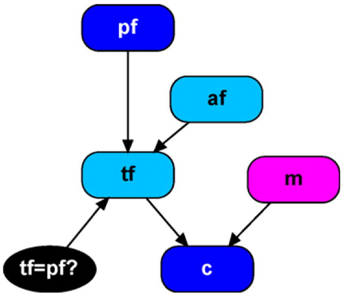
Simple disputed paternity network.

Rather than describe the entire network in detail, the reader is referred to Section 4 of [28] where all nodes and network classes are described. Here, a brief summary of the notation is given, then we explain the variations needed to account for allelic dependencies. Table 1 provides descriptions for each node in Fig. 1. A founder is any individual, either observed or unobserved, required to complete the necessary pedigree for a given case. In this example, the putative father and mother are observed founders as we have their genotype data, whereas the potential alternative father is an unobserved founder.

Table 1.

Node descriptions for Fig. 1

Node	Node type	Description
pf	Observed founder	Putative father
af	Unobserved founder	Alternative father
tf	Query	True father
m	Observed founder	Mother
c	Observed child	Child
tf=pf?	Hypothesis	Is the putative father the true father?

Throughout, we use the term allele to refer to the particular form of a gene. A gene such as vWA has several different allelic forms and it is an allele that is transmitted from parent to child. As the distinction between gene and allele was not made in [28], the node labeling here will differ. Another important difference between the treatment here, and that of [28] is that we restrict allele nodes to have a maximum of five states. We still permit loci with any number of alleles, we are simply making use of the fact that the mother and putative father could have at most four distinct alleles between them. Thus, we use the following numerical states for all allele nodes: 1 = generic label for first allele observed; 2 = label for the second distinct allele observed; 3 = label for the third distinct allele; 4 = label for the fourth distinct allele; 99 = label representing a pooling of all other non-observed alleles. In the case where we do not observe four distinct alleles, we simply assign probability zero to the superfluous states. To illustrate, suppose we observe four A₁ alleles. We then assign A₁ the generic label of 1 and we set the probability of an allele node taking on state 1 to be population allele frequency for A₁. We then set the probability of having states 2–4 equal to zero, and set the probability of state 99 equal to 1 minus the probability of state 1. These state definitions ensure our networks are generalizable for any loci with any number of alleles. They also serve to constrain the size of conditional probability tables (thus reducing computational complexity) when using loci with many allelic states.

Note that because of this simplification our networks here cannot handle the additional complications of mutations and silent alleles in the same way as they are addressed in [28]. In Section 5, we will address this distinction between the allele node definitions in more detail.

The new network for the simple paternity case which incorporates allelic dependencies appears in Fig. 2. For reference, Appendix A contains a tabular description of the entire network structure, in object-oriented programming terms. In addition, an enlarged network illustration is included, which shows the details of how information is passed among the modules. The following sections describe in detail four network classes that have been introduced: allele counter, update counts, unobserved founder, parameters. The remaining network classes (founder, allele, genotype, query, child and meiosis) are taken directly from [28], noting that our allele node is equivalent to their gene node.

Fig. 2.

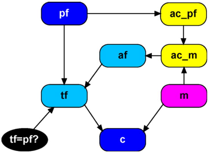
Simple disputed paternity network with allelic dependencies.

3.1. Allele counter and update counts

The first modification is to add two instances of the allele counter network class and they are labeled ac_pf and ac_m in Fig. 2. The internal structure of these modules appears in Fig. 3. This module counts how many of each allele is observed, supplying the network with the appropriate values for n_i as required by Eq. (3). The input variables a1 and a2 (input nodes are marked by an outer grey band accompanied by a dotted outline) represent the two alleles observed from the specified founder. For example, suppose we are within the ac_pf module. The input alleles are exact replicas of the putative father’s observed alleles. The input variables n_A1_in- n_A4_in represent the current counts for each allele. That is, they are numeric variables that can potentially take on any value from 0,…, n where n is the total number of alleles observed. If no initial values are passed in to the module (as is the case for ac_pf) the default state is 0 with probability one.

Fig. 3.

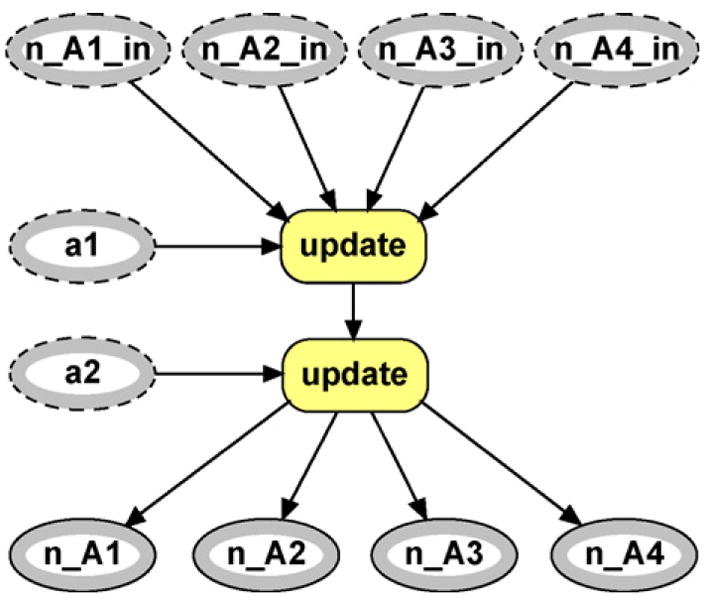
Allele counter module.

The first input allele and the input counting nodes are passed to another module labeled update which is an instance of the update counts network class which is shown in Fig. 4. This module takes existing counts as inputs and increases the appropriate count based on which allele is observed. In this first instance, the initial counts are set to zero as mentioned earlier within the allele counter class. The output nodes (marked by an outer grey band accompanied by a solid outline) will be updated according to the allele observed. For example, if the observed allele ais ‘3’ then the output node n_A3_out will take on the value 1 + n_A3_in, which in this case is 1 (since all input nodes are initialized to zero). All other output nodes will take on the values of their input nodes, in this case 0.

Fig. 4.

Update counts module.

The output nodes from the first update module are then passed to the next update module as input nodes, along with a2, and the counts are then updated with the second observed allele. For example if we again observe a ‘3’ allele, then the output node n_A3_out will take on the value 1 + n_A3_in, which is 2 since we have now observed two ‘3’ alleles. This updating concludes by passing the final counts to the output variables of the allele counter module, labeled n_A1,…, n_A4.

These counting nodes then become the input nodes for the next allele counter module, labeled ac_m. This module will update the counts in exactly the same fashion as above, but now according to the genotype observed for the mother. Once the final counts for all observed alleles are tallied, they are then passed on to the unobserved founder module so that the allele frequencies for af can be calculated using Eq. (3).

It is important to emphasize that the ordering of the counting nodes is arbitrary. The likelihood ratio is unaffected if first we count the mother’s alleles and then the putative father’s. This arises as the allele counts for all observed individuals are tallied before making use of them (via Eq. (3)) when determining the alleged father’s allele frequencies.

3.2. Founder and unobserved founder

The structure of the founder module is left unchanged from [28] and it is shown in Fig. 5. The new unobserved founder module appears in Fig. 6. The first difference between the founder network class and the unobserved founder class is that there are now input nodes corresponding to the allele counter module’s output nodes. In addition, p_in and m_in instances of the allele network class have been removed. This is due to the fact that the allele frequencies for p and m are no longer simply the population allele frequencies as specified in the allele class. They are now calculated based on Eq. (3), which necessitates the introduction of the new module shown in Fig. 6, parameters (labeled par).

Fig. 5.

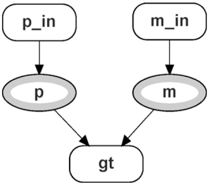
Founder module.

Fig. 6.

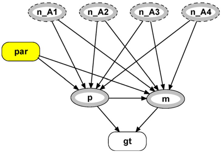
Unobserved founder module.

3.3. Parameters

Several parameter values employed by Eq. (3) are stored within the parameters module. There is no structure to this module per se, as it is just a collection of independent nodes representing θ, p_i, and n (shown in Fig. 7). Population allele frequencies are represented in Fig. 7 by the nodes p1, p2, p3, p4. These are numeric nodes with only one state (thus required to have probability 1) which is the value of that allele’s frequency in the population. Housing these nodes within the parameters module means that when reusing the network for other loci or other examples the allele frequencies need to be updated in only one place within the network.

Fig. 7.

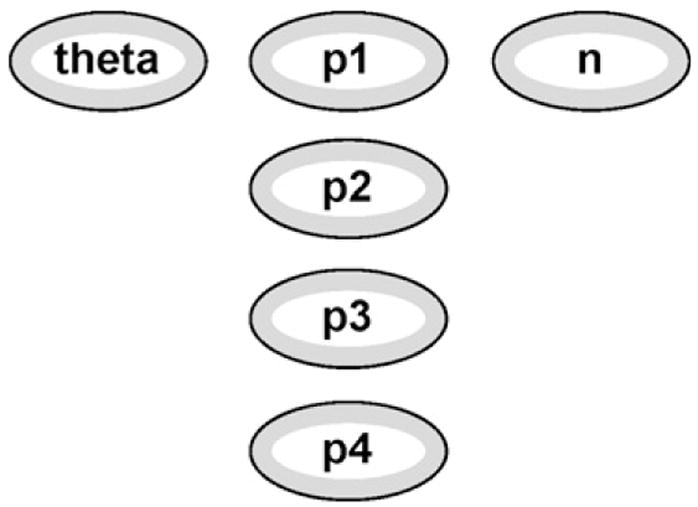
Parameters module.

The node theta is also numeric, taking on one state that corresponds to the coancestry coefficient appropriate for the given case. Finally, n is a numeric node specifying the total number of alleles we observe in the network (n from Eq. (3)). In this simple paternity case, we will observe n = 4alleles, two from the mother and two from the putative father. Ideally, the value of this node would be determined at run-time as the sum of the input counting nodes. This would unnecessarily complicate the representation of the network. Thus for illustration purposes, we have the user set it as a constant.

Each node in the parameters module will serve as input nodes for both p and m (nodes within the unobserved founder module). It is important to note here one of the limitations of the object-oriented framework within HUGIN: links are not allowed to cross into more than one level of nested modules. Consider the input variables n_A1,…, n_A4 from the unobserved founder module. It would be more sensible to house these nodes within the parameters module as they are parameters utilized by Eq. (3), and as they determine explicitly the value for n. However, this would require a link from the outer main network to cross through the unobserved founder module and into the parameter module, which is not permitted with this version of HUGIN.

Returning to the unobserved founder module, we have described the function of the n_Ai and par nodes. Let us now consider the probability tables associated with p and m. These nodes represent the paternal and maternal alleles of the unobserved founder. The node p has five states and a formula can be defined for each state, using the expression feature of HUGIN. The formulas for the first four states are P_4,n1 (A₁), P_4,n2 (A₂), P_4,n3 (A₃), and P_4,n4 (A₄) as defined by Eq. (3). The formula for state 99 is simply one minus the probabilities obtained for the other alleles.

There is nothing inherent in our network that requires the input counting nodes ( n_Ai) to add up to the number of alleles we have observed. Thus, their sum could potentially add up to a value greater than n. To ensure that HUGIN accurately calculates paternity index values, we must perform a check when specifying the probabilities for this node. If the input counting nodes sum to less than or equal to it n, then the formula we describe above will hold (as will always be the case). Otherwise, we (arbitrarily) specify a uniform distribution for the probabilities.

As mentioned, this is a superficial check, indeed a cumbersome ‘work-around’ dictated by structural limitations of HUGIN, since at no time will we observe any more than n alleles. An ideal solution computationally would be to store these values in an 1 × 4 array (the 4 is due to there being four distinct alleles possible, not n = 4 observed alleles) where the index represents the allele, and the value is the count of that allele at any given time. Unfortunately, this type of data structure does not exist within HUGIN. One could, however, make use of HUGIN’s API facility to maintain these counts and feed them into the appropriate nodes at run time. This would greatly simplify the representation, as the allele counter and update counts modules become unnecessary.

The conditional probability table for m is complicated by the additional dependence it will have on the node p. The value of n must be increased to five, and n_i must be updated according to which paternal allele is assigned. It should be noted that the m and p labels are selected solely for descriptive purposes. We are not implying that the paternal allele somehow ‘comes before’ the maternal one. Quite simply, one allele must be assigned first so that the allele frequencies of the other can be updated accordingly. It is helpful at this point to designate the p node as a model node for m within HUGIN. This allows the specification of different formulas for each state of p. For example, when p is in state 1 the formula for the probability that m is also 1 is P_{5, n1+1} (A₁). The same superficial check for the counting nodes described earlier is also employed here to ensure accurate results.

3.4. Paternity index calculations

Once the network is created, HUGIN can calculate the paternity index for various combinations of evidence. For example, consider the case where the mother’s genotype is A₁A₃, the putative father’s genotype is A₂A₄, and the child’s genotype is A₁A₂. First we must specify the prior odds of paternity as one in the tf=pf? node by entering a probability of 0.50 for the two alternatives, true and false. This ensures that the posterior odds do in fact equal the likelihood ratio. Then we compile the network and submit the evidence by entering the appropriate gtmin and gtmax values for pf (2, 4), m (1, 3), and c (1, 2). The posterior probabilities for the tf=pf? node calculated by HUGIN appear in Fig. 8. If we then divide the percentages (81.10 by 18.90) we obtain the paternity index value, 4.29. Evett and Weir [6] show the following is the PI formula for this case,

Fig. 8.

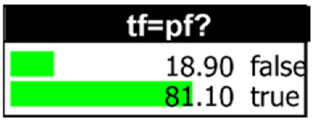
Posterior probabilities for tf=pf? .

$$\text{PI}=\frac{1+3\theta }{2[\theta +(1-\theta )p_2]}.$$ (5)

When θ = 0.03 and p₂ = 0.1, this formula gives PI = 4.29 which corresponds to HUGIN’s result.

4. Example two: Paternity case with missing father

Here we consider the more complex situation that can occur when forensic scientists do not have access to the putative father’s DNA. Instead, suppose they have a sample from a relative of the putative father. In particular, consider the case when DNA is available from a brother of the putative father. An object-oriented network depicting this situation is provided in Fig. 9. In this example we have three unobserved founder nodes, gf, gm, afrepresenting the parents of the putative father, and the alternative father. The node pf is changed to an (unobserved) child node as his parents now appear in our model. The node b represents the putative father’s brother and is an (observed) child node. All of the other nodes in the network remain unchanged from the presentation in the previous example.

Fig. 9.

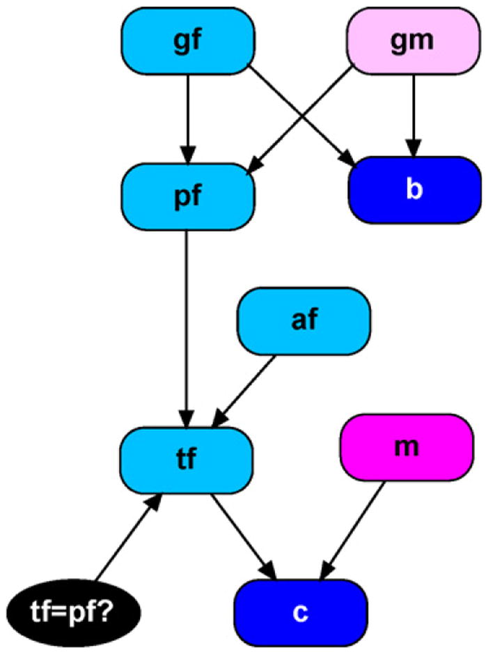
Missing putative father paternity network.

Incorporating allelic dependencies requires allele counter nodes to be added to this network, similar to those added in the previous example. First, we add ac_gf which counts the alleles observed in the grandfather’s genotype. This information is then be passed to the unobserved founder node gm, as the updated counts are needed to calculate appropriate allele frequencies. Next, we add ac_gm to include the grandmother’s alleles in the counts. Finally, ac_m is added to count the alleles observed by the mother. These new counts, tallying the alleles observed at gf, gm, and m are then passed to the alternative father, so that his allele frequencies are calculated according to Eq. (3) within the unobserved founder module. A representation of this new network appears in Fig. 10.

Fig. 10.

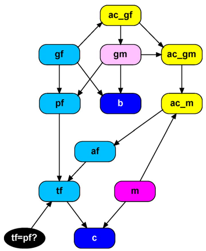
Missing putative father paternity network with allelic dependencies.

As there are now up to six alleles observed, each counting node in the network must have seven states, corresponding to the counts 0, 1,…, 6. This has greatly increased the complexity of the network, and as a result the GUI interface of HUGIN is no longer able to compile the network due to lack of memory. This seems reasonable, as the size of the combined conditional probability tables (CPT) for the first example was 23,414, whereas the CPT size for the network in Fig. 10 is now 1,564,221. It can however handle this example if we limit our data to biallelic loci. A discussion of how to forge ahead when faced with the complexities introduced by adding many unobserved founders is discussed in Section 5.

4.1. Biallelic missing father case

The network shown in Fig. 10 is easily modified to allow for only two alleles. The state space for every allele node in the network is reduced, now having only two states, either 1 or 2. In addition, the allele counter module is now responsible for tallying just two alleles, as opposed to all 4 alleles as illustrated in Fig. 3. Similarly, the update module shown in Fig. 4 is reduced to only five nodes, n_A1_in, n_A2_in, g, n_A1_out, and n_A2_out. The n_A3 and n_A4 nodes are removed from the unobserved founder module shown in Fig. 6. Finally, within the parameter module, the nodes p3and p4 are removed.

The resulting network is easily compiled in HUGIN and can be used to report the likelihood ratios for a given set of observations. This scenario was examined very early on by [30] and it later appeared in [6]. The likelihood ratio in this case is sometimes referred to as the Avuncular Index (AI), as opposed to the paternity index. The plaintiff’s new hypothesis is that tested man is a paternal uncle of the child. The defense hypothesis contends that the tested man is unrelated to the child. A simple mathematical relationship between the paternity index and the avuncular index is given by Eq. (6)[30],

$$\text{AI}=\left(\frac{1}{2}\right)\text{PI}+\frac{1}{2}.$$ (6)

Suppose we observe the mother’s genotype as A₁A₁, the brother’s genotype as A₁A₂, and the child’s genotype as A₁A₁. observed genotypes from the putative father, mother and child. If instead of observing A₁A₂ for the brother, we in fact observed it as the putative father’s genotype, the paternity index would be 2.91 [6], assuming θ = 0.03, p₁ = 0.10 and p₂=0.90. Thus, according to Eq. (6), we should obtain the AI shown in Eq. (7),

$$\text{AI}=\left(\frac{1}{2}\right)\text{(2}\text{.91)}+\frac{1}{2}=\mathrm{1.96.}$$ (7)

This result is obtained from HUGIN using our biallelic version of the network shown in Fig. 10. Once the observed data is entered, HUGIN displays posterior percentages for the hypothesis node tf=pf? as 66.18 for “true” and 33.82 for “false,” verifying the AI of 1.96.

5. Discussion

The networks presented in this paper provide graphical representations for various paternity cases, and also provide a computational alternative to sometimes laborious hand calculations. Unfortunately, additional functionality must be afforded before Bayesian networks are to remain valuable tools to the forensic scientist. The most likely scenarios in which Bayesian networks would prove invaluable are very complex cases with several observed and unobserved founders in a pedigree. These are the cases where hand calculation is nearly impossible and a computational tool is required. Unfortunately these are also the cases where the methods as proposed here break down. Additional research is needed into the use of HUGIN’s Application Programming Interface which is a promising solution to many of the problems encountered here. For example, additional data structures can be exploited when HUGIN is used in conjunction with other programming languages. This would be especially useful when tallying the number of observed genes, as required by Balding and Nichols’ method.

Another disadvantage of the methods presented here are the limiting assumptions. Specifically, assuming the population allele frequencies and θ values are known is particularly disconcerting. As mentioned earlier, this is rarely the case. An area for future research is to investigate relaxing these assumptions, and allowing for uncertainty in their values. The hierarchical nature of Bayesian networks and the programming interface provided by HUGIN will prove especially useful in this research, as Monte Carlo simulation techniques could be used to incorporate uncertainty in these estimates.

As mentioned earlier, the networks here differ from those presented in [28] in the specification of the state space for allele nodes. In [28], the number of states was dictated by the locus being used in the analysis. For example, they compute the likelihood ratios for various cases using the vWA locus which has a total of 11 alleles, thus their gene nodes all have a 11 states. Due to the additional complexity introduced by accounting for allelic dependence we decided here to reduce the number of states to the smallest possible number, while still ensuring the networks were generalizable to all loci. Unfortunately, this means that the modifications presented in [28] to handle silent alleles and mutation do not directly apply to the networks presented here. However, if the additional complexity introduced by multiple allelic states can be handled more efficiently with the API, then this will no longer be an issue. In addition, a simple line of code could alter the number of allelic states for every gene node in the network, thus automating the process of switching between different loci.

As a final note, it may be the case that the individuals involved may not belong to the same subpopulation. If it is reasonable to consider the subpopulations as independent, a simple extension to the methods proposed here could be employed. One could introduce separate counting nodes for each subpopulation under consideration. For example, if the putative father and the (potential) alternative father are believed to from a distinct subpopulation from that of the mother, then her allele counts would be handled by another counting mechanism specifically for her subpopulation. Thus observing her alleles would not affect the allele frequencies for the subpopulation of the alternative father and would then be ignored. It is possible to allow for dependence among subpopulations; the reader is referred to [31].

6. Conclusion

Bayesian Networks have become a useful tool for DNA evidence evaluation. They allow scientists to point and click their way to solutions to at times very laborious probability calculations. HUGIN and its promising application programming interface make these networks relatively simple to create and easy to use for the programmer. Here, we have presented an extension of an already established graphical tool to further empower the forensic scientist. The networks presented here are in no way ideal, perfect solutions to the problem. Instead, they should be viewed as a stepping stone to more complex and robust methods that are sure to follow.

Before the power of Bayesian networks can be fully utilized by the forensic scientist, a purpose-built software program must be created, designed to meet their needs. Specifically, this software must be able to appropriately handle a diverse range of scenarios that can arise in forensic identification cases including mixtures, mutations, silent alleles, and indeed population structure. The research presented here, and continued research in this area will perfect these representations, ensuring correct implementation by any future software engineers.

Appendix A

See Table A.1 and Fig. A.1.

Table A.1.

Module and node descriptions for the OOBN shown in Fig. 2

Class name	Class description	Input	Output	Class members
Main	Computes paternity index for simple paternity case	N/A	N/A	Founder ( pf, m), Unobserved Founder ( af), Query ( tf), Child ( c), Allele Counter ( ac_pf, ac_m)
Founder	Represents the genotype of an observed individual	None	p m	Allele ( pin, min), Genotype ( gt)
Allele	Represents one allele	None	allele	None
Genotype	Obtains the paternal and maternal alleles of an individual and converts them observable alleles by assigning max and min	p m	gtmin gtmax	None
Unobserved founder	Represents the genotypes of an unobserved individual assigning allele frequencies according to Eq. (3)	n_A1 n_A2 n_A3 n_A4	p m	Parameters ( par), Counts ( c), Genotype ( gt)
Parameters	Maintains the values of n, pi, and θ needed to calculate allele frequencies for unobserved founders	None	theta p1 p2 p3 p4 n	None
Counts	Ensures that the allele counts do not add up to a number larger than the total number of observed alleles	n_A1_in n_A2_in n_A3_in n_A4_in	n_A1_out n_A2_out n_A3_out n_A4_out	None
Query	Assigns alleles to true father, depending on value of pf=tf?	pfp pfm afp afm	tfp tfm pf=tf?	None
Child	Assigns alleles to child in line with maternal and paternal genotypes	fp fm mp mm	p m	Meiosis ( fmeiosis, mmeiosis), Genotype ( gt)
Meiosis	Mimics Mendelian inheritance	p m	c	None
Allele counter	Updates allele counting nodes by counting observed genes	a1 a2	n_A1 n_A2 n_A3 n_A4	Update Counts ( update×2)
Update counts	Increases counts according to allele ( a)	n_A1 n_A2 n_A3 n_A4 a	n_A1_out n_A2_out n_A3_out n_A4_out	None

Fig. A.1.

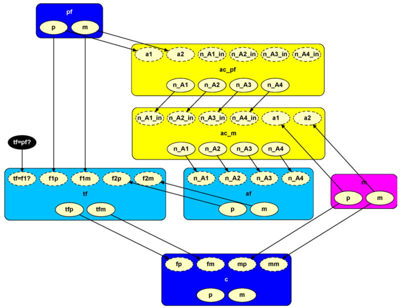
Expanded simple paternity Network for incorporating allelic dependence.

References

- 1.Taroni F, Aitken C, Garbolino P, Biedermann A. Bayesian Networks and Probabilistic Inference in Forensic Science. John Wiley and Sons; Chichester: 2006. [Google Scholar]
- 2.Weir BS. Effects of inbreeding on forensic calculations. Annu Rev Genet. 1994;28:597–621. doi: 10.1146/annurev.ge.28.120194.003121. [DOI] [PubMed] [Google Scholar]
- 3.Curran JM, Buckleton JS, Triggs CM. What is the magnitude of the subpopulation effect? Forensic Sci Intl. 2003;135(1):1–8. doi: 10.1016/s0379-0738(03)00171-3. [DOI] [PubMed] [Google Scholar]
- 4.Curran JM, Buckleton JS. The appropriate use of subpopulation corrections for differences in endogamous communities. Forensic Sci Intl. 2007;168(2–3):106–111. doi: 10.1016/j.forsciint.2006.06.073. [DOI] [PubMed] [Google Scholar]
- 5.Curran JM, Triggs CM, Buckleton JS, Weir BS. Interpreting DNA mixtures in structured populations. J Forensic Sci. 1999;44(5):987–995. [PubMed] [Google Scholar]
- 6.Evett IW, Weir BS. Interpreting DNA Evidence. Sinauer; Sunderland, MA: 1998. [Google Scholar]
- 7.Essen-Möller E. Die beweiskraft der ähnlichkeit im vaterschaftsnachweis: Theoretische grundlagen. Mitteilungen der Anthropologischen Gesellschaft. 1938;68:9–53. [Google Scholar]
- 8.Gill P, Foreman L, Buckleton JS, Triggs CM, Allen H. A comparison of adjustment methods to test the robustness of an STR DNA database comprised of 24 European populations. Forensic Sci Intl. 2003;131:184–196. doi: 10.1016/s0379-0738(02)00423-1. [DOI] [PubMed] [Google Scholar]
- 9.Balding DJ, Nichols RA. DNA profile match probability calculation—how to allow for population stratification, relatedness, database selection and single bands. Forensic Sci Intl. 1994;64(2–3):125–140. doi: 10.1016/0379-0738(94)90222-4. [DOI] [PubMed] [Google Scholar]
- 10.National Research Council. The Evaluation of Forensic DNA Evidence. National Academy Press; Washington, DC: 1996. [Google Scholar]
- 11.Balding DJ, Greenhalgh M, Nichols RA. Popullation genetics of STR loci in Caucasians. Int J Legal Med. 1996;108:300–305. doi: 10.1007/BF02432124. [DOI] [PubMed] [Google Scholar]
- 12.Buckleton JS, Curran JM, Walsh SJ. How reliable is the subpopulation model in DNA testimony. Forensic Sci Intl. 2006;157:144–148. doi: 10.1016/j.forsciint.2005.04.004. [DOI] [PubMed] [Google Scholar]
- 13.Cowell RG, Dawid AP, Lauritzen SL, Spiegelhalter DJ. Probabilistic Networks and Expert Systems. Springer-Verlag; Berlin-Heidelberg-New York: 1999. [Google Scholar]
- 14.Fenton N, Neil M. The jury observation fallacy and the use of Bayesian networks to present probabilistic legal arguments. Math Today. 2000;36(6):180–187. [Google Scholar]
- 15.Korb K, Nicholson A. Bayesian Artificial Intelligence. Chapman & Hall CRC Press; Boca Raton, FL: 2004. Appendix B available at http://www.csse.monash.edu.au/bai/book/appendix_b.pdf. [Google Scholar]
- 16.Evett IW, Gill PD, Jackson G, Whitaker J, Champod C. Interpreting small quantities of DNA: the hierarchy of propositions and the use of Bayesian networks. J Forensic Sci. 2002;47(3):520–530. [PubMed] [Google Scholar]
- 17.Dawid AP, Mortera J, Pascali VL, Boxel DV. Probabilistic expert systems for forensic inference from genetic markers. Scand J Stat. 2002;29:577–595. [Google Scholar]
- 18.Mortera J. Analysis of DNA mixtures using Bayesian networks. In: Green PJ, Hjort NL, Richardson S, editors. Highly Structured Stochastic System. Oxford University Press; 2003. pp. 39–44. [Google Scholar]
- 19.Aitken C, Taroni F, Garbolino P. A graphical model for the evaluation of cross-transfer evidence in DNA profiles. Theor Popul Biol. 2003;63:179–190. doi: 10.1016/s0040-5809(03)00004-2. [DOI] [PubMed] [Google Scholar]
- 20.Cowell RG. FINEX: A probabilistic expert system for forensic identification. Forensic Sci Int. 2003;134:196–206. doi: 10.1016/s0379-0738(03)00164-6. [DOI] [PubMed] [Google Scholar]
- 21.Taroni F, Biedermann A, Garbolino P, Aitken C. A general approach to Bayesian networks for the interpretation of evidence. Forensic Sci Int. 2004;139(1):5–13. doi: 10.1016/j.forsciint.2003.08.004. [DOI] [PubMed] [Google Scholar]
- 22.Biedermann A, Taroni F, Delemont O, Semadeni C, Davison A. The evaluation of evidence in the forensic investigation of fire incidents. Part 1: an approach using Bayesian networks. Forensic Sci Int. 2005;147(1):49–57. doi: 10.1016/j.forsciint.2004.04.014. [DOI] [PubMed] [Google Scholar]
- 23.Taroni F, Bozza S, Biedermann A. Two items of evidence, no putative source: an inference problem in forensic intelligence. J Forensic Sci. 2006;51(6):1350–1361. doi: 10.1111/j.1556-4029.2006.00272.x. [DOI] [PubMed] [Google Scholar]
- 24.Cavallini D, Corradi F. Forensic identification of relatives of individuals included in a database of DNA profiles. Biometrika. 2006;93(3):525–536. [Google Scholar]
- 25.Koller D, Pfeffer A. Object-oriented Bayesian networks. Proceedings of the 13th Annual Conference on Uncertainty in Artificial Intelligence (UAI-97); Morgan Kaufmann, San Francisco, CA. 1997. pp. 302–331. [Google Scholar]
- 26.Laskey K, Mahoney S. Network fragments: representing knowledge for constructing probabilistic models. Proceedings of the 13th Annual Conference on Uncertainty in Artificial Intelligence (UAI-97); Morgan Kaufmann, San Francisco, CA. 1997. p. 334. [Google Scholar]
- 27.Dawid AP. In: Bishop CM, Frey BJ, editors. An object-oriented Bayesian network for estimating mutation rates; Ninth International Workshop on Artificial Intelligence and Statistics; Key West, Florida. 2003. [Google Scholar]
- 28.Dawid AP, Mortera J, Vicard P. Object-oriented Bayesian networks for Q1 complex forensic DNA profiling problems. Forensic Sci Int. doi: 10.1016/j.forsciint.2006.08.028. in press. [DOI] [PubMed] [Google Scholar]
- 29.Buckleton JS. Population genetic models. In: Buckleton JS, Triggs CM, Walsh SJ, editors. Forensic DNA Evidence Interpretation. CRC Press; Boca Raton, FL: 2005. pp. 65–122. [Google Scholar]
- 30.Morris JW, Garber RA, d’Autremont J, Brenner CH. The avuncular index and the incest index. Adv Forensic Haemogenet. 1988;1:607–611. [Google Scholar]
- 31.Gary J, Beecham W, Weir BS. Confidence interval of the likelihood ratio Q2 associated with mixed stain dna evidence. doi: 10.1111/j.1556-4029.2010.01600.x. submitted for publication. [DOI] [PMC free article] [PubMed] [Google Scholar]