Determination of binding constants by affinity capillary electrophoresis, electrospray ionization mass spectrometry and phase-distribution methods

Abstract

Many methods for determining intermolecular interactions have been described in the literature in the past several decades. Chief among them are methods based on spectroscopic changes, particularly those based on absorption or nuclear magnetic resonance (NMR) [especially proton NMR (¹H NMR)]. Recently, there have been put forward several new methods that are particularly adaptable, use very small quantities of material, and do not place severe requirements on the spectroscopic properties of the binding partners. This review covers new developments in affinity capillary electrophoresis, electrospray ionization mass spectrometry (ESI-MS) and phasetransfer methods.

1. Introduction

Non-covalent intermolecular associations are omnipresent in chemical and biochemical systems. Cyclodextrin-drug inclusion, and protein-drug, peptide-peptide, carbohydrate-drug and antigen-antibody binding are a few examples. Binding constants provide a fundamental measure of the affinity of a solute to a ligand; hence the determination of binding constants has been an important step in describing and understanding molecular interactions.

Many techniques have been developed to measure binding constants. They can be categorized into two groups: separation-based; and, non-separation-based methods [1].

Separation-based methods physically separate the free solute and the bound solute, and evaluate their concentrations. Depending on how the separation is achieved, they can be further classified as heterogeneous or homogeneous. Chromatography [2], dialysis [3], ultrafiltration [4], surface-plasmon resonance (SPR) [5] are heterogeneous methods. The free solute is separated from the bound one on the surface of a solid substrate. Affinity capillary electrophoresis (ACE) [6-9] and electrospray ionization mass spectrometry (ESI-MS) [10] are homogeneous methods. The separation occurs either in solution or in the gas phase.

Non-separation-based methods monitor the change in specific physicochemical properties of the solute or ligand upon complexation. This category includes: spectroscopy (e.g., ultraviolet-visible (UV-Vis) [11-13], infrared (IR) [14], fluorescence [13,14], and nuclear magnetic resonance (NMR) [15]); electrochemical methods (e.g., conductimetry [15], potentiometry [16], and polarography [17]); and, phase-solubility [18] and hydrolysis kinetics [19,20].

Connors [21] thoroughly reviewed many of the above methods 20 years ago, hence this selective review will emphasize ACE, ESI-MS, and phase-distribution methods recently.

2. Affinity capillary electrophoresis

ACE refers to the separation by CE of substances that participate in specific or non-specific affinity interactions during CE [22]. In the past two decades, ACE has been one of the most rapidly growing analytical techniques for studying a variety of non-covalent interactions and determining binding constants and stoichiometries.

There have been specialized and general reviews of ACE [6,9,22-49] Most of them covered progress and innovation in ACE during a certain period with respect to biological-based molecular interactions. Other topics include combinatorial library screening [28], chiral additive evaluation [40], and cyclodextrin-drug inclusion [35,40]. Detection-sensitivity improvement [31] and miniaturization [48] are also continuing foci for technological innovations within ACE. There have been several reviews of the theoretical aspect of ACE [9,23,24,26,31,37,46,47], including a discussion of the advantages and the limitations of various ACE methods [24,26,31,46].

ACE may be classified in three modes:

In dynamic equilibrium ACE, the binding-equilibrium relaxation time is short with respect to the separation time. In this mode, the complex is in equilibrium with unbound (or free) solute and ligand.

In pre-equilibrated ACE, solute and ligand are first combined off-column, allowed to equilibrate, then introduced into the separation capillary. In this mode, the complex is long-lived compared to the separation time. The complex and free solute (or ligand) present as separate peaks (if a small volume of the equilibrated solution is injected).

In between are found so-called kinetic methods. In this mode, the relaxation time of the equilibrium is similar to the separation time. The analysis by Horvath's group of the effect of the timescale of a unimolecular reaction (cis-trans isomerization) on the CE separation is relevant to understanding the differences between these modes of ACE [50,51].

2.1. Dynamic-equilibrium ACE (rapid kinetics)

Related methods include mobility-shift ACE, Hummel-Dreyer (HD), vacancy ACE (VACE) [52,53], and vacancy-peak (VP) methods. We discuss below details of experimental design and data analysis for each method. Except for VACE, the methods were primarily developed for high-performance liquid chromatography (HPLC) and transferred to CE. These methods can be subdivided according the way the binding constants are determined from the change of the electrophoretic mobility of the species (mobility-shift ACE and VACE) or from the solute (free and bound) concentration evaluated by the peak area (HD and VP).

Dynamic-equilibrium ACE methods assume that the equilibrium between the solute and the ligand is established very quickly in the capillary. Most studies also assume that the stoichiometry of the binding between the target and the ligand is 1:1 to establish a simple model (see below). Complex formation by the solute (S) and the ligand (L) with the binding constant (K_1:1) is described by the following equation:

$$S+L\stackrel{K_{1:1}}{\rightleftharpoons }SL$$ (1)

Hence the binding constant is:

$$K_{1:1}=\frac{\left[SL\right]}{\left[S\right]\cdot \left[L\right]}$$ (2)

where [S], [L], and [SL] are the concentrations of the free solute, free ligand, and solute-ligand complex.

In mobility-shift ACE, a capillary is filled with buffer containing L in varying concentrations and a small amount of S is injected. Two peaks may appear in the electropherogram, as shown in Fig. 1.1a. The positive peak corresponds to the injected S (both free and bound). The migration time of this peak is monitored for the calculation of μ_i, the apparent electrophoretic mobility of S, expressed as:

$${\mu }_i=\frac{\left[S\right]}{\left[S\right]+\left[SL\right]}{\mu }_f+\frac{\left[SL\right]}{\left[S\right]+\left[SL\right]}{\mu }_c$$ (3)

where μ_f and μ_c are the electrophoretic mobilities of the free solute and solute-ligand complex, respectively.

Figure 1.

Simulated electropherograms of the methods: (A) mobility-shift ACE (HD); (B) VP (VACE) (adapted from [24], with permission from Elsevier).

Similarly, in VACE, the capillary is filled with a buffer containing both S and L. The concentration of either S or L is fixed and the concentration of the other component is varied. The presence of S and L in the capillary causes a large background response in the detector. After a small plug of neat buffer is injected, the voltage is switched on and two negative peaks (Fig. 1.1b) will appear in the electropherogram corresponding to free S and L caused by the decrease in their local concentrations. The change in mobility of the vacancy peak is treated as the solute peak in ACE. From Equation 2, Equation 3 can be written as:

$${\mu }_i=\frac{{\mu }_f+{\mu }_c{K}_{1:1}\left[L\right]}{1+K_{1:1}\left[L\right]}$$ (4)

Equation 4 can be converted into:

$$\left({\mu }_i-{\mu }_f\right)=\frac{\left({\mu }_c-{\mu }_f\right)K_{1:1}\left[L\right]}{1+K_{1:1}\left[L\right]}$$ (5)

Electrophoresis under conditions where such an equilibrium exists can be simulated [54]. For example, concentration-distance profiles can lead to an understanding of the underlying processes. Note that these simulations are based on mass balance, not charge balance. As long as the analytes are sufficiently dilute, this is acceptable. For an accurate assessment of behavior in the more general case, consideration of charge balance is needed [55,56].

Evaluation of experimental data is easier when Equation 5 is rearranged into a linear form, such as double reciprocal plot:

$$\frac{1}{\left({\mu }_i-{\mu }_f\right)}=\frac{1}{\left({\mu }_c-{\mu }_f\right)K_{1:1}}\cdot \frac{1}{\left[L\right]}+\frac{1}{\left({\mu }_c-{\mu }_f\right)}$$ (6)

If the solute has a much smaller concentration than the ligand, then [L] can be approximated 1 by [L_tot], which is the total concentration of the ligand. Hence by plotting $\frac{1}{\left({\mu }_i-{\mu }_f\right)}$ versus $\frac{1}{\left[L_{tot}\right]}$, the y intercept will give the value of$\frac{1}{\left({\mu }_c-{\mu }_f\right)}$, and K_1:1 = intercept / slope.

Equation 5 can be converted into other linear forms, such as the y-reciprocal plot:

$$\frac{\left[L\right]}{\left({\mu }_i-{\mu }_f\right)}=\frac{1}{\left({\mu }_c-{\mu }_f\right)}\cdot \left[L\right]+\frac{1}{\left({\mu }_c-{\mu }_f\right)\cdot K_{1:1}}$$ (7)

and the x-reciprocal plot:

$$\frac{\left({\mu }_i-{\mu }_f\right)}{\left[L\right]}=-K_{1:1}\cdot \left({\mu }_i-{\mu }_f\right)+K_{1:1}\left({\mu }_c-{\mu }_f\right)$$ (8)

All these linearization methods have different statistical weights of data points, which are shown in Table 1.

Table 1.

Equations used in affinity capillary electrophoresis (ACE) and variances in the transformed y for different calculation methods (adapted from [52,53])

Calculation methods	Equations	$${\sigma }_{y^{\prime }}^2$$
${\sigma }_{y\prime }^2$ is the variance of the transformed y; ${\sigma }_y^2$ is the variance in (μi − μf); the weight for each point is equal to $1∕{\sigma }_{y\prime }^2$
Non-linear regression	$$\left({\mu }_i-{\mu }_f\right)=\frac{\left({\mu }_c-{\mu }_f\right)K_{1:1}\left[L\right]}{1+K_{1:1}\left[L\right]}$$	$${\sigma }_y^2$$
Double reciprocal	$$\frac{1}{\left({\mu }_i-{\mu }_f\right)}=\frac{1}{\left({\mu }_c-{\mu }_f\right)K_{1:1}}\cdot \frac{1}{\left[L\right]}+\frac{1}{\left({\mu }_c-{\mu }_f\right)}$$	$$\frac{{\sigma }_y^2}{({\mu }_i-{\mu }_f{)}^4}$$
y-reciprocal	$$\frac{\left[L\right]}{\left({\mu }_i-{\mu }_f\right)}=\frac{1}{\left({\mu }_c-{\mu }_f\right)}\cdot \left[L\right]+\frac{1}{\left({\mu }_c-{\mu }_f\right)\cdot K_{1:1}}$$	$$\frac{[L{]}^2\cdot {\sigma }_y^2}{({\mu }_i-{\mu }_f{)}^4}$$
x-reciprocal	$$\frac{\left({\mu }_i-{\mu }_f\right)}{\left[L\right]}=-K_{1:1}\cdot \left({\mu }_i-{\mu }_f\right)+K_{1:1}\cdot \left({\mu }_c-{\mu }_f\right)$$	$${\left(K_{1:1}+\frac{1}{\left[L\right]}\right)}^2\cdot {\sigma }_y^2$$

However, generally, non-linear regression is more accurate and precise for the estimation of binding constants than linear regressions following algebraic manipulation (e.g., inverse plots) [57,58]. Bowser and Chen considered how to derive accurate values of K from data [59,60]. In all cases, it is necessary to use a range of concentrations over which “bound” and “free” concentrations change significantly. Also, the sensitivity of the analysis to binding influences the results. When one of the mobilities is altered significantly by binding, the resulting binding constant is more accurate. While non-linear regression is preferred for the best determination of K_1:1, one linearization, the x-reciprocal plot, can reveal the presence of complexes other than the 1:1 [61]. Detailed discussions of these important aspects of deriving an equilibrium constant from data are available [9,26,58-60]. It has recently been shown that an experimental design approach can be used to determine efficiently what conditions lead to accurate binding constants [62].

An alternate approach is to determine the equilibrium constant based on the concentrations of free and bound solute, as determined by their peak (or VP) area in HD and VP methods.

In the HD method, a capillary is filled with buffer containing S and a small amount of L dissolved in the run buffer is injected. Similarly, two peaks may appear in the electropherogram, as shown in Fig. 1.1a. The negative peak is caused by the local deficiency of S in the buffer, and the peak area is directly related to the concentration of S bound to L. Through either internal or external calibration [23], [SL] can be determined and [S] can also be obtained. For example, in an internal calibration, a series of samples with a fixed L concentration and increasing S concentrations are injected, and, by plotting the peak area versus the S concentration, the x-intercept gives the value of [SL] [23]. Since the L concentration is much less than the S concentration, the stoichiometry can be estimated by dividing [SL] by [L_tot]. This is one of the specific advantages of the HD method.

In the VP method, the experimental protocol is the same as for VACE, outlined above. The VP method uses the area of the VP corresponding to free S to construct the binding isotherm, and an internal calibration process is needed to determine [S]. [23]. Given [SL], [S], and [L_tot], and, since Equation 2 can be rearranged to:

$$\frac{\left[SL\right]}{\left[S\right]}=-K_{1:1}\left[SL\right]+K_{1:1}\left[L_{tot}\right]$$ (9)

the binding constant can be determined by plotting $\frac{\left[SL\right]}{\left[S\right]}$ versus [L^tot].

2.2. Pre-equilibrated (slow kinetics)

Similar to HD and VP methods, methods for pre-equilibrated sample mixtures (slow kinetics) give the equilibrium concentrations of the solute and the ligand from the electropherogram. Hence the binding constant can be determined according to Equation 2.

In the frontal analysis (FA) method, the capillary is filled with buffer and a large sample plug of pre-equilibrated S and L is injected. Depending on the dimensions of the capillaries, the sample volume is typically 20-200 nL (i.e. 5-20% of the total capillary volume) [46]. It is assumed that SL and L have approximately the same mobility and that the mobility of S differs significantly. Another assumption is that the dissociation rate of the complex is slow enough that it can be neglected. Upon application of the electrical field, free S begins to separate from the mixture. Two plateaus will be detected, as shown in Fig. 2. Plateau (a) corresponds to free S and plateau (b) corresponds to S + SL. Hence the concentration of free S can be determined from its plateau height through external calibration.

Figure 2.

Frontal analysis with capillary electrophoresis. Compounds: (·), solute; (○), ligand; (◉), soluteligand complex. A: Signal height reflecting the free solute concentration. B: Signal height reflecting the complex concentration (adapted from [9], with permission from Wiley and the author).

Frontal analysis-continuous CE (FACCE) differs from FA in the sample-introduction step. The capillary inlet is immersed in the sample vial during CE; hence continuous sample introduction is achieved. Apparently, FACCE requires free S to migrate faster than SL. As in the FA method, the plateau height corresponding to free S can be correlated to its concentration.

Affinity-probe CE (APCE) is a related pre-equilibration method. In this technique, a (fluorescently) labeled tag is used on one of the binding partners, typically the lower molecular-weight partner. This permits extension of ACE methods to more complex samples and lower concentrations because of the use of a label, resulting in access to a wider range of binding constants [63].

Even more selectivity is attained from using fluorescence anisotropy detection [64], in which a significant anisotropy clearly signals the ‘bound’ form of the relatively low-molecular-weight labeled compound. Another advantage, as long as a label is being used, is control of the charge in the labeled ligand to improve separation selectivity [65].

2.3. Kinetic methods (intermediate kinetics)

In the methods described so far, the characteristic equilibration time for the reaction is either much shorter than the residence time or greater than the residence time [51]. In kinetic CE, the timescales for separation and chemical relaxation are more similar. Considering the kinetics of the complex formation of S and L, Equation 1 can be rewritten as:

$$S+L\underset{k_{\mathrm{off}}}{\overset{k_{\mathrm{on}}}{\rightleftharpoons }}SL$$ (10)

where k_on and k_off are rate constants of complex formation and dissociation, respectively. Hence according to Equation 2:

$$K_{1:1}=k_{on}∕k_{off}$$ (11)

Early work by Whitesides [66] and Heegaard [67] showed the value of analyzing the peak shape when it is perturbed by a slow equilibrium. In Whitesides [66], both the change in electrophoretic mobility and the shape (but not the area) of the peak were used for the determination of k_on and k_off, and thus K_1:1.

Recently, Krylov has developed a series of kinetic CE methods by applying different experimental settings and data analysis approaches. Based on various initial and boundary conditions - the way interacting species enter and exit the capillary - a number of kinetic CE methods have been designed. A thorough review of these methods was given in 2007 [68]. Here, we briefly describe one of the approaches with simple mathematics [i.e. non-equilibrium CE of equilibrium mixtures (NECEEM)].

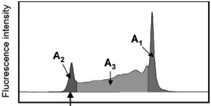
In NECEEM, a buffer is used as the background electrolyte. A short plug of the equilibrium mixture of S and L is injected into the inlet of the capillary, and complex SL continuously dissociates during CE. If the separation of S, L, and SL is efficient, re-association of S and L can be neglected. Hence the resulting electropherogram contains three peaks, as shown in Fig. 3, representing S, L, and SL, and two exponential “smears” of S and L, which occur from the dissociation of SL. Fig. 4 shows an experimental NECEEM electropherogram for the interaction between fluorescently-labeled ssDNA and SSB protein. The dissociation constant and rate, K_d and k_off, respectively, can be calculated as:

$$K_d=1∕K_{1:1}=\frac{\left[S{]}_0\right(1+A_1∕\left(A_2+A_3\right))-[L{]}_0}{1+\left(A_2+A_3\right)∕A_1}$$ (12)

$$k_{off}=\ln \left(\frac{A_2+A_3}{A_1}\right)∕t_{SL}$$ (13)

where A₁ is the peak area corresponding to L, A₂ is the peak area corresponding to SL, which was still intact at the time it passed through the detector, A₃ is the area of the exponential smear left by L dissociated from SL during the separation, and, finally, t_SL is the migration time of the complex. [S]₀ and [L]₀ are total concentrations of S and L in the equilibrium mixture.

Figure 3.

Simulated NECEEM electropherogram. A₁ is the peak area of L that was free in the equilibrium mixture (for NECEEM); A₂ is the peak area of intact SL at the time of its passing the detector; A₃ is the peak area of L dissociated from SL during the separation; and, t_L, t_SL, and t_S are migration times from the capillary inlet to the detector of L, SL, and S, respectively (adapted from [68], with permission from Wiley and the author).

Figure 4.

Experimental NECEEM electropherogram for the interaction between fluorescently-labeled ssDNA and SSB protein (reprinted from [68], with permission from Wiley and the author).

For NECEEM, as well as other kinetic CE methods, it is important to distinguish accurately the boundaries of the peaks. Two approaches have been proposed: a control experiment; and, mathematical modeling [68].

The boundary between A₁ and A₃ can be found by comparing the peaks of free L in the presence and absence of S [69]. However, experimental errors in the 10% range are inevitable [68].

In the mathematical approach, various parameters, including k_off, v_L, v_SL, D_L, D_SL and A₁ / (A₂ + A₃), are adjusted in regression analysis to minimize the deviation between experimental and simulated traces using the least-squares method [70]. Here v_L and v_SL are the electrophoretic velocities of L and SL, respectively; D_L and D_SL are the diffusion coefficients of L and SL, respectively. This modeling approach clearly requires effort. Nevertheless, compared to conventional ACE methods, NECEEM only needs a single run to determine the binding constants. A disadvantage of having the results derived from a single injection is the lack of an estimate for the error. Also, it is unwise to test models at only a single set of initial concentrations, so multiple measurements may be justified.

The availability of other methods based on various initial and boundary conditions makes kinetic CE a multi-method toolbox for not only measuring binding parameters but also testing hypotheses about interaction mechanisms [71]. Conceptually, experimental electropherograms are first obtained by multiple kinetic CE methods. A hypothetical model of interactions between S and L is suggested and electropherograms based on the hypothesis are simulated. The experimental kinetic CE electropherograms are compared with simulated ones to obtain the best fits. If the quality of the fit is unsatisfactory, a new hypothesis must be developed for the interaction. The procedure is repeated until a satisfactory hypothesis is found. The best fits for the accepted hypothesis lead to the determination of stoichiometric and kinetic parameters of the interaction [71].

2.4. Comparison of ACE methods

As a homogeneous, separation-based approach, ACE does not require immobilization of the ligand on a solid support with the risk of altering binding properties. Other advantages of ACE include low consumption of sample and reagent, and study of interactions near physiologically relevant conditions with respect to pH, ionic strength, and temperature. There are a number of experimental approaches for the determination of binding constants with ACE. Each exhibits specific ranges of applicability, advantages and limitations, so they can often be considered complementary rather than competitive.

Mobility-shift ACE has specific advantages compared to other approaches:

1. the injected sample need not be highly purified; and,

2. binding constants of several samples can be determined simultaneously.

However, the fluctuation of the electroosmotic flow (EOF) may adversely influence the observed electrophoretic mobility, so careful control or correction of EOF is needed. If the EOF is changing because of changes in zeta potential, coating of the capillary inner wall may be used to control EOF and to avoid solute adsorption on the inner wall of the capillary that may cause peak broadening and inaccurate mobility measurement. Alternatively, the mobility ratio (M) can be used to estimate binding constants [72]:

$$M={\mu }_{net}∕{\mu }_{eof}=(\mu +{\mu }_{eof})∕{\mu }_{eof}$$ (14)

where μ, μ_net, and μ_eo are the observed mobility, net mobility and electroosmotic mobility, respectively.

$$\frac{\Delta M}{\left[L\right]}=K_{1:1}\Delta M^{\max }-K_{1:1}\Delta M$$ (15)

where ΔM is the change in migration ratio as a function of [L], and ΔM^max is the maximum change in migration ratio that can be achieved with the saturation of L for complexation. This analysis method is independent of the capillary length, the applied voltage, and the EO mobility. If the EOF is changing because the buffer viscosity is changing, then a correction for the viscosity change is required, as the change in viscosity will not only alter the electroosmotic mobility, but also affect the solute and ligand electrophoretic mobilities [73].

In addition, the accuracy of mobility-shift analysis depends on the stability of the complex relative to the separation time. The complex-dissociation half-time, expressed as ln2/k_off, must be less than 1% of the peak-appearance time [74]. When the on and off rates are too slow to ensure establishment of a dynamic equilibrium, broadened, split, undetectable peaks may be observed [67]. This rule holds true for other dynamic equilibrium approaches (i.e. HD, VP, and VACE).

For methods that use the change in peak area or plateau height for the determination of the concentrations of free and bound solute, and thus the binding constant, special care must be taken to assure that the total-solute concentration is known accurately, since the bound-solute concentration is usually calculated as the difference between the total and free concentrations of the solute. It is therefore assumed that no solute is lost due to capillary-wall adsorption or any other non-specific phenomena (e.g., precipitation) [75] and that the concentration in the sample corresponds to the concentration during CE (i.e. no stacking occurs), or at least any loss is corrected based on a standard curve obtained under identical conditions [46]. These requirements are more restrictive than those applied for mobility-shift ACE.

In contrast with dynamic equilibrium ACE, FA and FACCE usually require the complex to be quite stable, so that a subsequent quantitation of the free S plateau height reflects the free S concentration in the sample. For molecular interactions characterized by relatively rapid binding kinetics, the validity of using these two approaches should be verified. This may be accomplished by inspection of both ascending and descending solute boundaries [76], which is possible in FA but not FACCE. These two methods are suitable for measuring K_1:1 values in the range 10³−10⁸/M [77]. For weak interactions, the height difference between the two frontal zones may be too small. In this case, mobility-shift ACE may be preferred for the determination of binding constant. If K_1:1 is too large, the plateau height for free S may be too small to be measured [37].

An attractive feature of FA and FACCE is that they are insensitive to changes or fluctuations in migration times, EOF and applied voltage [78]. Low detection limit is also an advantage of these two methods.

Compared to FA, FACCE requires greater sample consumption (e.g., 500 nL) [79] but is supposedly advantageous since continuous sampling may avoid perturbation of the binding equilibrium [80]. Moreover, FACCE usually provides a broader plateau than FA, and that may be easier for quantitation [46].

One of the requirements for FA and FACCE is that the mobilities of L and SL must be equal; otherwise, the free S plateau does not reflect the true free-solute concentration at equilibrium [24,76]. This may potentially limit application of FA and FACCE. The mobility requirements for other ACE methods (i.e. mobility-shift ACE, HD, VP and VACE) have been thoroughly discussed, as has various approaches to studying multiple equilibriums [24].

Kinetic CE methods can determine K_1:1, k_off, and k_on from a single CE experiment when 1:1 binding stoichiometry has been verified. One of the most attractive features of kinetic CE is that it is a multi-method tool based on various initial and boundary conditions; hence some proposed affinity mechanisms for a specific approach can be validated by a series of comparison studies. A potential problem of kinetic CE is the difficulty in distinguishing the equilibrium fractions of corresponding components, which may lead to uncertainty in the estimate of the binding parameters [46]. The applications of kinetic CE methods to higher order equilibriums are also expected.

There are certainly some inherent limitations to all ACE methods for evaluating binding constants. For instance, it may be difficult to evaluate the association of two or more neutral molecules. In addition, with a few exceptions [73,81], applications of ACE have not been extended to interaction studies in non-aqueous solvents [9].

3. Electrospray ionization mass spectrometry

ESI-MS provides a soft ionization procedure that allows the transfer of weakly-bound complexes from solution to the gas phase for mass analysis, so it has frequently been used to study the binding behavior of a wide variety of non-covalent complexes [82-84]. Specificity, sensitivity, and speed are advantages of ESI-MS [85]. Moreover, ESI-MS can provide stoichiometric information of the complex directly and detect multiple components simultaneously.

Since one of the earliest reviews that discussed the potential of using ESI-MS to study non-covalent complexes [86], many reports have reviewed the application of ESI-MS in various binding studies (e.g., binding of drugs, metals, and proteins to DNA [87], protein complexes [88], host-guest interactions [82]), most of which focused on the determination of the identity of complexes, but not the quantitative aspects of their formation.

To determine the binding constant of a complex quantitatively through ESI-MS, one of the most frequently used approaches is titration. Generally, the solute concentration in the solution is kept constant while the ligand concentration is varied over a range of about two orders of magnitude [85]. The gas-phase-ion intensities of the free and bound solute are monitored, and can be fitted to association models for calculation of binding constants.

We consider a 1:1 system:

$$K_{1:1}=\frac{\left[SL\right]}{\left[S\right]\cdot \left[L\right]}=\frac{\left[SL\right]}{\left[S\right]\cdot \left(\left[L_{tot}\right]-\left[SL\right]\right)}$$ (16)

where [L_tot] is the total concentration of the ligand.

Since:

$$\left[SL\right]=\left[S_{tot}\right]\cdot \frac{\left[SL\right]}{\left[S\right]+\left[SL\right]}$$ (17)

Equation 16 can be converted into:

$$K_{1:1}=\frac{\left[SL\right]}{\left[S\right]}\cdot \frac{1}{\left[L_{tot}\right]-\left[S_{tot}\right]\cdot \frac{1}{\frac{\left[S\right]}{\left[SL\right]}+1}}$$ (18)

Define:

$$\frac{\left[S\right]}{\left[SL\right]}=\frac{i_S∕f_S}{i_{SL}∕f_{SL}}=\frac{i_S}{i_{SL}}\cdot \frac{f_{SL}}{f_S}=IF$$ (19)

where i_S and i_SL are the ion intensities of the free and bound solute, respectively; f_S and f_SL are the response factors of the free and bound solute, respectively. Hence Equation 18 can be converted into:

$$\left(IF{)}^2{K}_{1:1}\right[L_{tot}]+IF(K_{1:1}\left[L_{tot}\right]-K_{1:1}\left[S_{tot}\right]-1)-1=0$$ (20)

Equation 20 can be further converted into various forms, for determining K_1:1.

The ratio of ion intensities (I) can be obtained from the mass spectrum for each concentration point. However, there is no valid method that is suitable for determining the response factor of the complex (f_SL) and thus the ratio of response factors (F). It is often assumed that the response factors of the free and bound solutes are similar, and then F can be approximated to unity. However, different molecular species may undergo different vaporization and ionization efficiencies. Response factors may also change with pH, further complicating quantitation [89]. This represents one of the biggest disadvantages of the ESI-MS method for binding-constant determination [90]. The influence of response factors has been discussed in detail [91]. In addition, ESI is not an instantaneous process, so changes can occur when non-covalent complexes are transferred from solution phase to gas phase. For instance, when the kinetics of dissociation is on the same timescale as the evaporation process, evaporation of the droplet can cause displacement of the complexation equilibrium towards association [84]. However, the evaporation process is rapid enough to be a factor for fast reactions only [92]. A recent experimental measurement confirmed that droplet shrinking does not influence monomer-dimer equilibrium of a fluorescent dye. Control experiments demonstrated that dye concentrations increased in droplets as their size decreased [93].

Recent studies on biological [94] and inorganic [89] systems concluded that the ESI-MS approach was useful for quantitative measurements of binding constants. However, a close reading shows that confidence in a quantitative result is warranted only if there is already available a considerable amount of information on the system.

The limitations of the ESI-MS method described above can be improved partly by competition approaches. Basically, a reference compound is mixed with the solute for complexation with the ligand. The reference should have a similar structure to the solute and its binding behavior with the ligand should be known. The binding constant between solute and ligand can therefore be indirectly obtained by comparing the two binding systems [85]. In other cases, stable complexes with similar structures can be added as internal standards for the estimation of response factors [95]. From a practical point of view, ESI-MS should be used to determine relative binding affinities (selectivities) rather than absolute values.

4. Phase-distribution methods

Phase-distribution methods monitor the dependence of the solute-distribution coefficient between two phases on the ligand concentration in one phase to determine the solute-ligand binding constant. Usually, one of the phases is aqueous and the other is organic. The binding equilibrium can be studied in either phase. This method has been applied to measure binding constants for the complex formation of caffeine/benzoic acid [18], solute/cyclodextrin [2,96-103], metal ion/anion [104], and drug/chiral selector [105].

Equation 1 describes the formation of 1:1 complex. For consecutive complexation:

$$\mathrm{S}-{\mathrm{L}}_{i-1}+\mathrm{L}\stackrel{K_{1:i}}{\rightleftharpoons }\mathrm{S}-{\mathrm{L}}_i$$ (21)

The binding constant (K_1:i) is defined as:

$$K_{1:i}=\frac{[S\cdot L_i]}{[S\cdot L_{i-1}]\left[L\right]}$$ (22)

The distribution of the free solute between phase 1 and phase 2 is determined by partition ratio D₀:

$$D_0=\frac{[S{]}_1}{[S{]}_2}$$ (23)

where [S]₁ and [S]₂ are the free-solute concentrations in phase 1 and phase 2, respectively. When the ligand is added to phase 1, the solute-distribution coefficient is:

$$D=\frac{[S{]}_1+\sum _{i=1}^n[S\cdot L_i{]}_1}{[S{]}_2}$$ (24)

where n is the stoichiometry, [S-L_i] (i = 1 to n) is the concentration of solute-ligand complex in phase 1 in various forms. Dividing Equation 25 by Equation 24:

$$\frac{D}{D_0}=1+\sum _{i=1}^n\frac{[S\cdot L_i]}{\left[S\right]}$$ (25)

From Equation 23, one obtains:

$$[S\cdot L_i]=\left[S\right][L{]}^i\underset{j=1}{\overset{i}{\Pi }}{K}_{1:j}$$ (26)

Here:

$$K_{1:j}=\frac{[S\cdot L_j]}{[S\cdot L_{j-1}]\left[L\right]}$$ (27)

Inserting Equation 27 into Equation 26:

$$\frac{D}{D_0}=1+\sum _{i=1}^n\left([L{]}^i\underset{j=1}{\overset{i}{\Pi }}{K}_{1:j}\right)$$ (28)

Plotting D/D₀ versus [L], the stoichiometry and the binding constants can be obtained from polynomial fitting analyses. A similar, but algebraically more complex, approach is required if the ligand exists in various states of protonation.

The phase-distribution method provides an option for measuring binding constants for complex formation. Advantages of this method include relatively low sample requirement, availability to measure binding constants under physiological conditions (e.g., pH, temperature and ionic strength) and the potential to utilize high-throughput screening technologies [105,106].

However, there are several disadvantages that have to be taken into consideration. The mutual solubility of the two phases may interfere and complicate the binding equilibrium. It is even possible that some organic solvent may function as a competitor to bind the ligand (e.g., octanol/cyclodextrin) [103], which should be carefully investigated to prevent misinterpretation of the calculated binding parameters [2]. In addition, all species present in phase 1 (e.g., free solute, free ligand and complexes) may partition to the second phase. The model described above assumes the partitioning of only the free solute, so it has been over-simplified.

Octanol has been the most frequently used solvent as the organic phase in phase-distribution studies. In this case, entrainment and emulsion can be severe problems when very hydrophobic compounds are studied [107].

4.1. High-throughput phase-distribution method based on solid-phase microextraction

One of the most important strategies in the pharmaceutical field is to reduce the time and the labor needed for research and development of new drugs. This has led to the movement of pharmaceutical and biotechnology companies toward high-throughput screening (HTS) of small-molecule compounds for their discovery programs [108]. More compounds have become available for further investigations. Consequently, high-throughput technologies are demanded in the post-synthetic stages in the research and development process.

Recently, a high-throughput phase-distribution method was introduced for the determination of octanol/water partitioning [109], chirally discriminating binding [105] and drug-cyclodextrin binding [110]. Taking the last study as an example of the approach, as shown in Fig. 5, drug substances were prepared in plasticized poly(vinyl) chloride (PVC) films (plasticizer: dioctyl sebacate (DOS)) in a high-throughput manner; buffer solution containing a particular cyclodextrin was then added, and the amount of drug extracted to the aqueous phase was determined by HPLC for the calculation of drug-cyclodextrin binding constant. This method used solid-phase microextraction (SPME), and had certain advantages compared with other phase-distribution methods (e.g., better reproducibility, shorter equilibration time, and easier automation) [111]. In addition, entrainment and emulsion problems could be eliminated. The same approach was also used to determine drug-chiral selector binding constants [105] and octanol-water partition coefficients [110]. With respect to the latter, for a set of reference compounds, the partition coefficients of the solutes in the PVC-DOS/water system were equal to those in octanol/water, so the technique provides a direct measure of log P_ow.

Figure 5.

General procedure of the high-throughput phase-distribution method to determine the binding constant of drug to cyclodextrin.

5. Conclusions

Some general conclusions are warranted. All the methods described have the advantage of using very little material. The phase-distribution method, especially in its high-throughput form, is advantageous in many regards. Of the three methods described above, it is the least dependent on models for deriving information from data. The analytical method used for quantitation is not defined by the approach - any suitable method can be used. Under many circumstances, all three methods can function with impurities. The phase-distribution method would not be appropriate, for the most part, for studies of protein-protein or metal-polar ligand binding, as the typical phases are aqueous and non-aqueous.

ACE methods are useful for cases where at least one of the binding partners is detectable with good mass-detection limits. There is a powerful ability to derive kinetic information as well as thermodynamic information when the timescales are appropriate. While not model-free, data analysis is straightforward. Further, a preliminary ACE result can be subjected to additional scrutiny by a second ACE approach that is particularly sensitive to a parameter (e.g., stoichiometry) that comes out of the preliminary analysis.

The power of the MS approaches lies in the ability to see all or many of the components of the mixture. This advantage is moderated somewhat by the presence of multiple-charge states (requiring deconvolution), assumptions about fragmentation reactions and, when proteins are involved, alterations in charge state brought about by changes in the structure of one of the partners.

In the future, it is possible to envision higher throughput for phase-distribution methods. Microplates with 1536 wells are available. Furthermore, diffusional relaxation is exceptionally well understood, so acquiring data before the system reaches equilibrium should provide information about the equilibrium. Throughput is the strength of the high-throughput phase-distribution approach.

ACE methods will grow. One may predict that the coupling of ACE methods with MS, so far used rarely and only for model studies [112,113], will increase. In complex, multi-component equilibriums, the qualitative identification power of MS will be more important the more partners there are in the complex.

As for the ESI-MS approach, there is a long way to go. Studies that focus on understanding the chemistry in the droplets produced by the spray using non-MS observations of the droplets (e.g., a fine study is [93]) will lay the foundation for relating ionization efficiency to instrumental and chemical conditions. Despite the difficulty of determining binding constants quantitatively by ESI-MS, the technique is nonetheless critical for the qualitative understanding of the distribution of the binding partners among several different forms in solution (bound/free, monomer/dimer, analyses of three-component systems, (A, B and C) to find A·B, A·C, B·C, A·B·C, and similar non-covalent complexes with other stoichiometries).

References

- [1].Klotz IM. Ligand-Receptor Energetics: A Guide for the Perplexed. John Wiley & Sons; New York, USA: 1997. [Google Scholar]
- [2].Masson M, Sigurdardottir BV, Matthiasson K, Loftsson T. Chem. Pharm. Bull. 2005;53:958. doi: 10.1248/cpb.53.958. [DOI] [PubMed] [Google Scholar]
- [3].Sideris EE, Georgiou CA, Koupparis MA, Macheras PE. Anal. Chim. Acta. 1994;289:87. [Google Scholar]
- [4].Kokugan T, Yudiarto A, Takashima T, Dewi E. J. Chem. Eng. Jpn. 1998;31:640. [Google Scholar]
- [5].Wikstroem A, Deinum J. Anal. Biochem. 2007;362:98. doi: 10.1016/j.ab.2006.12.009. [DOI] [PubMed] [Google Scholar]
- [6].Schou C, Heegaard NHH. Electrophoresis. 2006;27:44. doi: 10.1002/elps.200500516. [DOI] [PMC free article] [PubMed] [Google Scholar]
- [7].Schipper BR, Ramstad T. J. Pharm. Sci. 2005;94:1528. doi: 10.1002/jps.20380. [DOI] [PubMed] [Google Scholar]
- [8].Karakasyan C, Taverna M, Millot M-C. J. Chromatogr. 2004;A 1032:159. doi: 10.1016/j.chroma.2003.11.021. [DOI] [PubMed] [Google Scholar]
- [9].Rundlett KL, Armstrong DW. Electrophoresis. 2001;22:1419. doi: 10.1002/1522-2683(200105)22:7<1419::AID-ELPS1419>3.0.CO;2-V. [DOI] [PubMed] [Google Scholar]
- [10].Beni S, Szakacs Z, Csernak O, Barcza L, Noszal B. Eur. J. Pharm. Sci. 2007;30:167. doi: 10.1016/j.ejps.2006.10.008. [DOI] [PubMed] [Google Scholar]
- [11].Archontaki HA, Vertzoni MV, Athanassiou-Malaki MH. J. Pharm. Biomed. Anal. 2002;28:761. doi: 10.1016/s0731-7085(01)00679-3. [DOI] [PubMed] [Google Scholar]
- [12].Koopmans C, Ritter H. J. Am. Chem. Soc. 2007;129:3502. doi: 10.1021/ja068959v. [DOI] [PubMed] [Google Scholar]
- [13].Fini P, Catucci L, Castagnolo M, Cosma P, Pluchinotta V, Agostiano A. J. Incl. Phenom. Macrocycl. Chem. 2007;57:663. [Google Scholar]
- [14].Tang J, Luan F, Chen X. Biorg. Med. Chem. 2006;14:3210. doi: 10.1016/j.bmc.2005.12.034. [DOI] [PubMed] [Google Scholar]
- [15].Sheehy PM, Ramstad T. J. Pharm. Biomed. Anal. 2005;39:877. doi: 10.1016/j.jpba.2005.03.046. [DOI] [PubMed] [Google Scholar]
- [16].Kahle C, Holzgrabe U. Chirality. 2004;16:509. doi: 10.1002/chir.20068. [DOI] [PubMed] [Google Scholar]
- [17].Khan F, Khan F. J. Chin. Chem. Soc. 2005;52:569. [Google Scholar]
- [18].Higuchi T, Zuck DA. J. Am. Pharm. Assoc. (1912-1977) 1952;41:10. doi: 10.1002/jps.3030410106. [DOI] [PubMed] [Google Scholar]
- [19].Loukas YL. Pharm. Sci. 1997;3:343. [Google Scholar]
- [20].Loukas YL, Vraka V, Gregoriadis G. Int. J. Pharm. 1996;144:225. [Google Scholar]
- [21].Connors KA. Binding Constants. John Wiley & Sons., Inc.; New York, USA: 1987. [Google Scholar]
- [22].Heegaard NHH. J. Mol. Recogn. 1998;11:141. doi: 10.1002/(SICI)1099-1352(199812)11:1/6<141::AID-JMR410>3.0.CO;2-D. [DOI] [PubMed] [Google Scholar]
- [23].Busch MHA, Carels LB, Boelens HFM, Kraak JC, Poppe H. J. Chromatogr. 1997;A 777:311. doi: 10.1016/s0021-9673(97)00369-5. [DOI] [PubMed] [Google Scholar]
- [24].Busch MHA, Kraak JC, Poppe H. J. Chromatogr. 1997;A 777:329. [Google Scholar]
- [25].Rippel G, Corstjens H, Billiet HAH, Frank J. Electrophoresis. 1997;18:2175. doi: 10.1002/elps.1150181208. [DOI] [PubMed] [Google Scholar]
- [26].Rundlett KL, Armstrong DW. Electrophoresis. 1997;18:2194. doi: 10.1002/elps.1150181210. [DOI] [PubMed] [Google Scholar]
- [27].Shimura K, Kasai K-I. Anal. Biochem. 1997;251:1. doi: 10.1006/abio.1997.2212. [DOI] [PubMed] [Google Scholar]
- [28].Chu Y-H, Zang X, Tu J. J. Chin. Chem. Soc. 1998;45:713. [Google Scholar]
- [29].Colton IJ, Carbeck JD, Rao J, Whitesides GM. Electrophoresis. 1998;19:367. doi: 10.1002/elps.1150190303. [DOI] [PubMed] [Google Scholar]
- [30].Gao J, Mrksich M, Mammen M, Whitesides GM. Chem. Anal. 1998;146:947. [Google Scholar]
- [31].Guijt-Van Duijn RM, Frank J, Van Dedem GWK, Baltussen E. Electrophoresis. 2000;21:3905. doi: 10.1002/1522-2683(200012)21:18<3905::AID-ELPS3905>3.0.CO;2-4. [DOI] [PubMed] [Google Scholar]
- [32].Heegaard NHH, Kennedy RT. Electrophoresis. 1999;20:3122. doi: 10.1002/(SICI)1522-2683(19991001)20:15/16<3122::AID-ELPS3122>3.0.CO;2-M. [DOI] [PubMed] [Google Scholar]
- [33].Heegaard NHH, Nilsson S, Guzman NA. J. Chromatogr. 1998;B 715:29. doi: 10.1016/s0378-4347(98)00258-8. [DOI] [PubMed] [Google Scholar]
- [34].Heegaard NHH, Shimura K. In: Quantitative Analysis of Biospecific Interactions. Lundahl P, Greijer E, Lundqvist A, editors. Harwood Academic; New York, USA: 1998. pp. 15–34. [Google Scholar]
- [35].Larsen KL, Zimmermann W. J. Chromatogr. 1999;A 836:3. [Google Scholar]
- [36].Oravcova J, Lindner W. In: Quantitative Analysis of Biospecific Interactions. Lundahl P, Greijer E, Lundqvist A, editors. Harwood Academic; New York, USA: 1998. pp. 191–226. [Google Scholar]
- [37].Tanaka Y, Terabe S. J. Chromatogr. 2002;B 768:81. doi: 10.1016/s0378-4347(01)00488-1. [DOI] [PubMed] [Google Scholar]
- [38].Tseng W-L, Chang H-T, Hsu S-M, Chen R-J, Lin S. Electrophoresis. 2002;23:836. doi: 10.1002/1522-2683(200203)23:6<836::AID-ELPS836>3.0.CO;2-J. [DOI] [PubMed] [Google Scholar]
- [39].Vollmerhaus PJ, Tempels FWA, Kettenes-Van den Bosch JJ, Heck AJR. Electrophoresis. 2002;23:868. doi: 10.1002/1522-2683(200203)23:6<868::AID-ELPS868>3.0.CO;2-#. [DOI] [PubMed] [Google Scholar]
- [40].Blaschke G, Chankvetadze B. Drugs Pharm. Sci. 2003;128:175. [Google Scholar]
- [41].Berezovski M, Sergey N. Krylov. Anal Chem. 2005;77:1526. doi: 10.1021/ac048577c. [DOI] [PubMed] [Google Scholar]
- [42].Galbusera C, Chen DDY. Curr. Opin. Biotechnol. 2003;14:126. doi: 10.1016/s0958-1669(02)00020-4. [DOI] [PubMed] [Google Scholar]
- [43].Gayton-Ely M, Pappas TJ, Holland LA. Anal. Bioanal. Chem. 2005;382:570. doi: 10.1007/s00216-004-3033-z. [DOI] [PubMed] [Google Scholar]
- [44].Heegaard NHH. Electrophoresis. 2003;24:3879. doi: 10.1002/elps.200305668. [DOI] [PubMed] [Google Scholar]
- [45].Jia Z. Curr. Pharm. Anal. 2005;1:41. [Google Scholar]
- [46].Oestergaard J, Heegaard NHH. Electrophoresis. 2006;27:2590. doi: 10.1002/elps.200600047. [DOI] [PubMed] [Google Scholar]
- [47].Ruettinger H-H. Drugs Pharm. Sci. 2003;128:23. [Google Scholar]
- [48].Vlckova M, Stettler A, Schwarz M. J. Liq. Chromatogr. Rel. Technol. 2006;29:1047. [Google Scholar]
- [49].Zavaleta J, Chinchilla D, Brown A, Ramirez A, Calderon V, Sogomonyan T, Gomez FA. Curr. Anal. Chem. 2006;2:35. [Google Scholar]
- [50].Anurag CH, Rathore S. Electrophoresis. 1997;18:2935. doi: 10.1002/elps.1150181535. [DOI] [PubMed] [Google Scholar]
- [51].Ma S, Kalman F, Kalman A, Thunecke F, Horvath C. J. Chromatogr. 1995;A 716:167. doi: 10.1016/0021-9673(95)00555-2. [DOI] [PubMed] [Google Scholar]
- [52].Erim FB, Kraak JC. J. Chromatogr. 1998;B 710:205. doi: 10.1016/s0378-4347(98)00127-3. [DOI] [PubMed] [Google Scholar]
- [53].Busch MHA, Boelens HFM, Kraak JC, Poppe H. J. Chromatogr. 1997;A 775:313. [Google Scholar]
- [54].Fang N, Sun Y, Zheng J, Chen DDY. Electrophoresis. 2007;28:3214. doi: 10.1002/elps.200600662. [DOI] [PubMed] [Google Scholar]
- [55].Gas B, Hruska V, Dittmann M, Bek F, Witt K. J. Sep. Sci. 2007;30:1435. doi: 10.1002/jssc.200600502. [DOI] [PubMed] [Google Scholar]
- [56].Hruska V, Jaros M, Gas B. Electrophoresis. 2006;27:984. doi: 10.1002/elps.200500756. [DOI] [PubMed] [Google Scholar]
- [57].Rao J, Colton IJ, Whitesides GM. J. Am. Chem. Soc. 1997;119:9336. [Google Scholar]
- [58].Rundlett KL, Armstrong DW. J. Chromatogr. 1996;A 721:173. [Google Scholar]
- [59].Bowser MT, Chen DDY. J. Phys. Chem. 1998;A 102:8063. [Google Scholar]
- [60].Bowser MT, Chen DDY. J. Phys. Chem. 1999;A 103:197. [Google Scholar]
- [61].Bowser MT, Chen DDY. Anal. Chem. 1998;70:3261. doi: 10.1021/ac9713114. [DOI] [PubMed] [Google Scholar]
- [62].Hanrahan G, Montes RE, Pao A, Johnson A, Gomez FA. Electrophoresis. 2007;28:2853. doi: 10.1002/elps.200600523. [DOI] [PubMed] [Google Scholar]
- [63].Whelan RJ, Sunahara RK, Neubig RR, Kennedy RT. Anal. Chem. 2004;76:7380. doi: 10.1021/ac0489566. [DOI] [PubMed] [Google Scholar]
- [64].Yang P, Whelan RJ, Jameson EE, Kurzer JH, Argetsinger LS, Carter-Su C, Kabir A, Malik A, Kennedy RT. Anal. Chem. 2005;77:2482. doi: 10.1021/ac048307u. [DOI] [PubMed] [Google Scholar]
- [65].Yang P, Whelan RJ, Mao Y, Lee AW-M, Carter-Su C, Kennedy RT. Anal. Chem. 2007;79:1690. doi: 10.1021/ac061936e. [DOI] [PubMed] [Google Scholar]
- [66].Avila LZ, Chu YH, Blossey EC, Whitesides GM. J. Med. Chem. 1993;36:126. doi: 10.1021/jm00053a016. [DOI] [PubMed] [Google Scholar]
- [67].Heegaard NHH. J. Chromatogr. 1994;A 680:405. doi: 10.1016/0021-9673(94)85136-0. [DOI] [PubMed] [Google Scholar]
- [68].Sergey NK. Electrophoresis. 2007;28:69. [Google Scholar]
- [69].Berezovski M, Nutiu R, Li Y, Sergey NK. Anal. Chem. 2003;75:1382. doi: 10.1021/ac026214b. [DOI] [PubMed] [Google Scholar]
- [70].Okhonin V, Krylova SM, Sergey NK. Anal. Chem. 2004;76:1507–1512. doi: 10.1021/ac035259p. [DOI] [PubMed] [Google Scholar]
- [71].Petrov A, Okhonin V, Berezovski M, Sergey NK. J. Am. Chem. Soc. 2005;127:17104. doi: 10.1021/ja056232l. [DOI] [PubMed] [Google Scholar]
- [72].Kawaoka J, Gomez FA. J. Chromatogr. 1998;B 715:203. doi: 10.1016/s0378-4347(98)00161-3. [DOI] [PubMed] [Google Scholar]
- [73].Bowser MT, Sternberg ED, Chen DDY. Electrophoresis. 1997;18:82. doi: 10.1002/elps.1150180117. [DOI] [PubMed] [Google Scholar]
- [74].Horejsi V, Ticha M. J. Chromatogr. 1986;376:49. [Google Scholar]
- [75].Tao L, Kennedy RT. Electrophoresis. 1997;18:112. doi: 10.1002/elps.1150180121. [DOI] [PubMed] [Google Scholar]
- [76].Winzor DJ. Anal. Biochem. 2006;349:285. doi: 10.1016/j.ab.2005.11.028. [DOI] [PubMed] [Google Scholar]
- [77].McDonnell PA, Caldwell GW, Masucci JA. Electrophoresis. 1998;19:448. doi: 10.1002/elps.1150190315. [DOI] [PubMed] [Google Scholar]
- [78].Oestergaard J, Hansen SH, Jensen H, Thomsen AE. Electrophoresis. 2005;26:4050. doi: 10.1002/elps.200500287. [DOI] [PubMed] [Google Scholar]
- [79].Gao JY, Dubin PL, Muhoberac BB. Anal. Chem. 1997;69:2945. doi: 10.1021/ac970026h. [DOI] [PubMed] [Google Scholar]
- [80].Hattori T, Kimura K, Seyrek E, Dubin PL. Anal Biochem. 2001;295:158. doi: 10.1006/abio.2001.5129. [DOI] [PubMed] [Google Scholar]
- [81].Peddicord MB, Weber SG. Electrophoresis. 2002;23:431. doi: 10.1002/1522-2683(200202)23:3<431::AID-ELPS431>3.0.CO;2-O. [DOI] [PubMed] [Google Scholar]
- [82].Brodbelt JS. Int. J. Mass Spectrom. 2000;200:57. [Google Scholar]
- [83].Di Marco VB, Bombi GG. Mass Spectrom. Rev. 2006;25:347. doi: 10.1002/mas.20070. [DOI] [PubMed] [Google Scholar]
- [84].Di Tullio A, Reale S, De Angelis F. J. Mass Spectrom. 2005;40:845. doi: 10.1002/jms.896. [DOI] [PubMed] [Google Scholar]
- [85].Daniel JM, Friess SD, Rajagopalan S, Wendt S, Zenobi R. Int. J. Mass Spectrom. 2002;216:1. [Google Scholar]
- [86].Loo JA. Mass Spectrom. Rev. 1997;16:1. doi: 10.1002/(SICI)1098-2787(1997)16:1<1::AID-MAS1>3.0.CO;2-L. [DOI] [PubMed] [Google Scholar]
- [87].Beck JL, Colgrave ML, Ralph SF, Sheil MM. Mass Spectrom. Rev. 2001;20:61. doi: 10.1002/mas.1003. [DOI] [PubMed] [Google Scholar]
- [88].Heck AJR, van den Heuvel RHH. Mass Spectrom. Rev. 2004;23:368. doi: 10.1002/mas.10081. [DOI] [PubMed] [Google Scholar]
- [89].Di Marco VB, Bombi GG, Ranaldo M, Traldi P. Rapid Commun. Mass Spectrom. 2007;21:3825. doi: 10.1002/rcm.3292. [DOI] [PubMed] [Google Scholar]
- [90].Raji MA, Frycak P, Beall M, Sakrout M, Ahn JM, Bao Y, Armstrong DW, Schug KA. Int. J. Mass Spectrom. 2007;262:232. [Google Scholar]
- [91].Gabelica V, Galic N, Rosu F, Houssier C, De Pauw E. J. Mass Spectrom. 2003;38:491. doi: 10.1002/jms.459. [DOI] [PubMed] [Google Scholar]
- [92].Peschke M, Verkerk UH, Kebarle P. J. Am. Soc. Mass. Spectrom. 2004;15:1424. doi: 10.1016/j.jasms.2004.05.005. [DOI] [PubMed] [Google Scholar]
- [93].Wortmann A, Kistler-Momotova A, Zenobi R, Heine MC, Wilhelm O, Pratsinis SE. J. Am. Soc. Mass. Spectrom. 2007;18:385. doi: 10.1016/j.jasms.2006.10.010. [DOI] [PubMed] [Google Scholar]
- [94].Mathur S, Badertscher M, Scott M, Zenobi R. Phys. Chem. Chem. Phys. 2007;9:6187. doi: 10.1039/b707946j. [DOI] [PubMed] [Google Scholar]
- [95].Spasojevic I, Boukhalfa H, Stevens RD, Crumbliss AL. Inorg. Chem. 2001;40:49. doi: 10.1021/ic991390x. [DOI] [PubMed] [Google Scholar]
- [96].Eli W, Chen W, Xue Q. J. Inclusion Phenom. Macrocycl. Chem. 2000;38:37. [Google Scholar]
- [97].Andreaus J, Draxler J, Marr R, Hermetter A. J. Colloid Interface Sci. 1997;193:8. doi: 10.1006/jcis.1997.5045. [DOI] [PubMed] [Google Scholar]
- [98].Andreaus J, Draxler J, Marr R, Lohner H. J. Colloid Interface Sci. 1997;185:306. doi: 10.1006/jcis.1996.4556. [DOI] [PubMed] [Google Scholar]
- [99].Tachibana M, Furusawa M, Kiba N. J. Inclusion Phenom. Mol. Recognit. Chem. 1995;22:313. [Google Scholar]
- [100].Menges RA, Armstrong DW. Anal. Chim. Acta. 1991;255:157. [Google Scholar]
- [101].Nakai Y, Yamamoto K, Terada K, Horibe H. Chem. Pharm. Bull. 1982;30:1796. doi: 10.1248/cpb.31.3745. [DOI] [PubMed] [Google Scholar]
- [102].Nakai Y, Yamamoto K, Terada K, Horibe H. J. Inclusion Phenom. 1984;2:523. [Google Scholar]
- [103].Nakajima T, Sunagawa M, Hirohashi T. Chem. Pharm. Bull. 1984;32:401. [Google Scholar]
- [104].Xia Y, Friese JI, Moore DA, Rao L. J. Radioanal. Nucl. Chem. 2006;268:445. [Google Scholar]
- [105].Chen Z, Yang Y, Werner S, Wipf P, Weber SG. J. Am. Chem. Soc. 2006;128:2208. doi: 10.1021/ja058004x. [DOI] [PMC free article] [PubMed] [Google Scholar]
- [106].Chen Z, Lu D, Weber SG. J. Pharm. Sci. 2008 doi: 10.1002/jps.21396. DOI: 10.1002/jps.21396. [Published ?] [DOI] [PMC free article] [PubMed] [Google Scholar]
- [107].Poole SK, Poole CF. J. Chromatogr. 2003;B 797:3. [Google Scholar]
- [108].Eldridge GR, Vervoort HC, Lee CM, Cremin PA, Williams CT, Hart SM, Goering MG, O'Neil-Johnson M, Zeng L. Anal. Chem. 2002;74:3963. doi: 10.1021/ac025534s. [DOI] [PubMed] [Google Scholar]
- [109].Chen Z, Weber SG. Anal. Chem. 2007;79:1043. doi: 10.1021/ac061649a. [DOI] [PMC free article] [PubMed] [Google Scholar]
- [110].Ahmadzadeh H, Dovichi NJ, Krylov S. Meth. Mol. Biol. 2004;276:15. doi: 10.1385/1-59259-798-X:015. [DOI] [PubMed] [Google Scholar]
- [111].Krishnan TR, Ibraham I. J. Pharm. Biomed. Anal. 1994;12:287. doi: 10.1016/0731-7085(94)90001-9. [DOI] [PubMed] [Google Scholar]
- [112].Machour N, Place J, Tron F, Charlionet R, Mouchard L, Morin C, Desbene A, Desbene P-L. Electrophoresis. 2005;26:1466. doi: 10.1002/elps.200410213. [DOI] [PubMed] [Google Scholar]
- [113].Lynen F, Zhao Y, Becu C, Borremans F, Sandra P. Electrophoresis. 1999;20:2462. doi: 10.1002/(SICI)1522-2683(19990801)20:12<2462::AID-ELPS2462>3.0.CO;2-5. [DOI] [PubMed] [Google Scholar]