Mapping all-atom models onto one-bead Coarse Grained Models: general properties and applications to a minimal polypeptide model

Abstract

In the one and two beads Coarse Grained (CG) models for proteins, the two conformational dihedrals ϕ and ψ that describe the backbone geometry are no longer present as explicit internal coordinates, thus the information contained in the Ramachandran plot cannot be used directly. We derive an analytical mapping between these dihedrals and the internal variable describing the backbone conformation in the one(two) beads CG models, namely the pseudo-bond angle and pseudo-dihedral between subsequent Cαs. This is used to derive a new density plot that contains the same information as the Ramachandran plot and can be used with the one(two) beads CG models. The use of this mapping is then illustrated with a new one bead polypeptide model that accounts for transitions between α-helices and β-sheets.

1 Introduction

Coarse Grained (CG) models for proteins have become more and more popular in the last two decades, due to the necessity of simulating systems on the size scale of hundreds of nanometers and on the time scale of microseconds[1,2]. The seminal concept can be traced back to the seventies[3,4]: these simplified models for proteins are based on united-atom representations using one to six interacting centers (beads) for each amino acid. Four-to-six beads models represent explicitly the backbone atoms (Cα, N(H) and C(O)) with additional “beads” for the side chain and for the backbone carbonylic oxygen and the backbone hydrogen[5,6,7], and use the ϕ and ψ dihedrals formed by the backbone atoms C-N-Cα-C and N-Cα-C-N respectively as internal variables. Conversely, in one(two) bead(s) models only the Cα (and additional beads for the side chain) is (are) explicitly present (see fig. 1).

Figure 1.

Schematic representation of the coarse graining procedure. The internal coordinates (ϕ, ψ ω) and θ, α and the angles defining the CG geometry (τ, γ1; γ2) are reported.

The two-dimensional density plot of ϕ and ψ referring to a given Cα is called the Ramachandran map. This map is more dense in specific regions of the ϕ, ψ plane, each pertaining to a particular secondary structure. Other regions are “forbidden” due to the steric hindrance of the backbone atoms. Thus, the Ramachandran plot is a simple and immediate tool to check the reliability of a model protein. But, while this check can be directly done in four(-six) bead models, this is no longer possible in the one(two) beads models. In fact, in these models, the ϕ and ψ are no longer explicit internal variables and the description of the backbone geometry relies on different internal variables, i.e. the Cα-Cα-Cα angle θ and the Cα-Cα-Cα-Cα dihedral α (see fig. 1). So far, the problem of how to transfer the information contained in the Ramachandran plot to these simplified models has not been given any consideration. This is quite surprising, given the fact that one and two beads models have recently undergone rapid developments becoming more accurate and sophisticated [8,9,10,11,12,13,14,15].

In this paper we derive an analytical correspondence of the all-atom internal back-bone coordinates (ϕ,ψ) to the CG internal backbone coordinates (α, θ) that allows one to explicitly map the Ramachandran plot onto a new θ, α conformational density plot. The Force Field (FF) of the recent one and two beads CG models, are reconsidered on the basis of the θ, α map. As an illustration of these concepts, a new one-bead model for polypeptides is presented that accounts for helix to sheet secondary structure transitions.

2 Coarse Graining and mapping of the internal backbone coordinates

The procedure leading from an all-atom model to a one(two)bead CG model is schematically described in fig. 1. The bond length and the backbone bond-angle NH-Cα-CO display only small variation from the average values (τ = 111deg), and the peptide bond geometry is planar (ω = 180)¹, implying that the dihedral angles ϕ and ψ are basically the only free internal variables. In the CG description, the backbone conformation is determined by the bond angle between three subsequent Cαs and the dihedral between four subsequent Cαs. The bond angle with vertex Cα_i, (θ_i) depends only on the two adjacent dihedrals ϕ_i and ψ _i, whereas the dihedral between Cα_i−1 and Cα_i+2, namely α_i,i+1, depends on the four dihedrals ϕ_i,ψ_i,ϕ_i+1,ψ_i+1. Both θ and α depend parametrically on τ and on the two angles between the bonds Cα-Cα and Cα-CO or Cα-NH, which for trans conformation assume the almost constant values of γ1 = 20.7deg and γ1 = 14:7deg respectively (see fig. 1 for the definition of angles and dihedrals). The angle θ as a function of ϕ, ψ is given by the following formula²

$$\begin{array}{l}\text{cos}({\theta }_i)=\text{cos}(\tau )[\text{cos}\mathrm{\gamma }1\text{cos}\mathrm{\gamma }2-\text{sin}\mathrm{\gamma }1\text{sin}\mathrm{\gamma }2\text{cos}({\varphi }_i)\cos ({\psi }_i)]\\ -\text{sin}\mathrm{\gamma }1\text{sin}\mathrm{\gamma }2\text{sin}({\varphi }_i)\text{sin}({\psi }_i)+\text{sin}(\tau )[\cos ({\psi }_i)\text{sin}\mathrm{\gamma }1\text{cos}\mathrm{\gamma }2+\text{cos}({\varphi }_i)\text{cos}\mathrm{\gamma }1\text{sin}\mathrm{\gamma }2]\end{array}$$ (1)

For (ϕ,ψ) = (180, 180), (0; 0), (180, 0) and (0, 180) one has θ = τ + (γ1 +γ2), θ = τ −(γ1+γ2), θ = τ +(γ1−γ2) and θ = τ −(γ1−γ2) respectively. The first corresponds to the completely extended conformation, the others are planar but sterically forbidden or weakly allowed conformations (see below). The exact formula giving α explicitly as a function of the ϕ,ψ dihedrals is very complex, however a precision of a few percent can already be obtained at the linear order in γ1 and γ 2 (see the Supporting Information)

$${\alpha }_{i,i+1}=180+{\psi }_i+{\varphi }_{i+1}+\mathrm{\gamma }1\text{sin}({\psi }_{i+1})+\mathrm{\gamma }2\text{sin}({\varphi }_i)$$ (2)

This formula (with γ1 = γ2) was previously reported by Levitt[3].

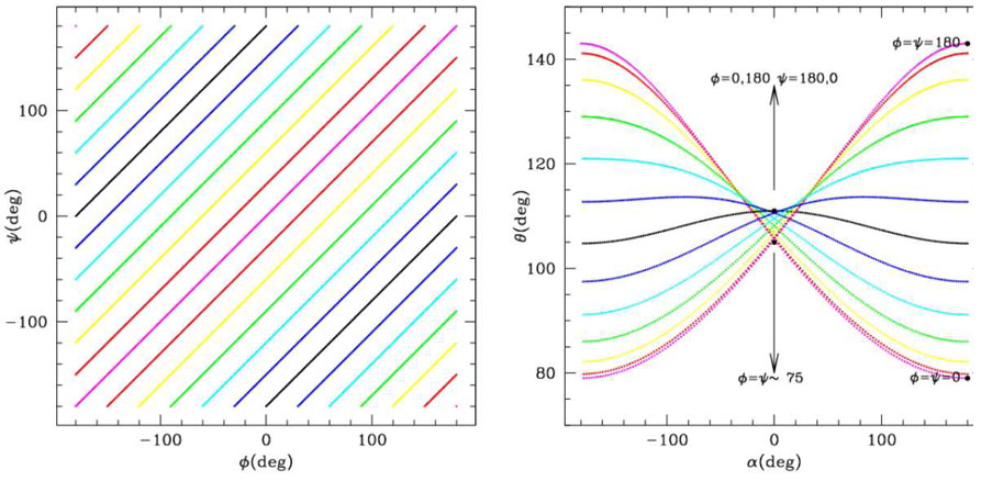
In order to make general considerations, we restrict ourselves to the case γ1 = γ2. Furthermore, we assume that the geometrical properties are uniform along the chain (or, equivalently, we consider cases of well defined secondary structure), so that we can put ϕ_i = ϕ_i+1 and ψ_i = ψ_i+1 and drop the dependence on the index i+1 in eqn (2). In these conditions, the map (ϕ,ψ) → (α, θ) is symmetric under the exchange ϕ ↔ ψ Thus the upper triangle in the (ϕ,ψ) plane is superimposed upon folding along the main diagonal (in magenta) over the lower triangle and mapped onto the same region in the α, θ plane. The periodicity and the additional symmetry θ (ϕ,ψ) = θ (− ϕ, −ψ) = θ (ϕ+180, ψ +180) determine the peculiar “butteryfly” shape of the image of the ϕ, ψ plane in the α, θ plane reported in fig. 2. In the general case when γ1 ≠γ2 the ϕ ↔ ψ symmetry is slightly broken and one has two slightly different “butterfly” images superimposed. It is to be noted that as the whole α axis is spanned, the θ angle can assume only values ranging between τ −γ1 −γ2 and τ + γ1 + γ2, corresponding to the planar-contracted (forbidden) configuration (ϕ = ψ = 0) and the planar extended configuration (ϕ = ψ = 180). As the angle α approaches the value 0, the allowed range for θ becomes smaller. Ring structures correspond to α = 0: the maximum value for θ is τ = 111 + |γ2 − γ1|, obtained for ϕ = 180deg,ψ = 0deg corresponding roughly to a six membered ring, while the minimum value for θ is ~ 105deg, obtained for ϕ = ψ ≃ ±75deg, corresponding roughly to a five membered ring.

Figure 2.

Mapping of the ϕ, ψ plane onto the θ, α plane. Left: lines ϕ−ψ =cost are represented in different colors. Right: The same lines are mapped onto the α, θ plane. The region that they define is the image of the whole ϕ, ψ plane onto the α, θ plane through the (ϕ, ψ) → (α, θ) map. Some relevant points are reported.

3 Conversion of the Ramachandran plot into the α, θ plot

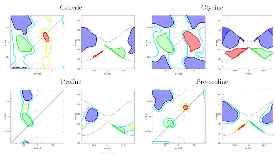
We use the above relationships to convert the Ramachandran plot into a conformational density plot in the α, θ plane. The conversion for the generic Ramachandran plot, the Ramachandran plot of Glycine, Proline and pre-proline residues are reported in fig. 3. We observe that the symmetry-induced folding of the ϕ,ψ plane along the diagonal produces some peculiarities of the α,θ conformational maps. For instance, the forbidden region around ϕ = ψ = 0 (simplified as a circle in fig. 3) is folded onto itself and mapped onto a flat region around α = ±180deg, θ = τ − γ1 − γ2 =≃ 75deg. Conversely, the forbidden region around ϕ = 0,ψ = ±180deg is folded on a weakly allowed region (ϕ = ±180, ψ = 0), implying that the corresponding region in the α, θ plane (represented as a small circle around α = 0, θ ≃ τ) is not strictly forbidden. The effect of the folding along the ϕ, ψ diagonal can be also seen on the core regions of the right handed (green) and left handed (red) regions, that are cut by the folding line. These assume peculiar folded and stretched shapes squeezed against the limits of the “butterfly” image. The same happens to the sheet region (blue) in the glycine plot. However, despite the folding and deformation of the Ramachandran plot, the core regions of the different secondary structures remain separate in the α, θ plane. This is important, since it implies that passing from the ϕ, ψ to the α, θ system of internal coordinates still allows an unambiguous description of the backbone conformation in each secondary structure. This was previously assumed in one and two beads CG models but never directly investigated.

Figure 3.

Mapping of the Ramachandran plot onto the α, θ plane for different aminoacid types. The “core regions” are in green (right handed helices), red (left handed helices), blue (sheets). The allowed regions (yellow and cyan) are omitted in the Generic and Glycine α, θ plot for clarity. Forbidden regions are enclosed in the dotted lines. The contours of the “butterfly” image are reported as black lines in the α, θ plane. The input data for the Ramachandran plot are taken from the Protein Data Bank[18].

In Table 1 the typical ϕ, ψ values for the main secondary structures are reported, as well as the corresponding α, θ values. We observe that right and left handed helices have the same value of θ and opposite values of α. Conversely, the θ variable is more effcient in separating the helices from the sheet structures, expecially in the glycine where both structures span almost the same α interval.

Table 1.

Numerical values of the internal angles and dihedral coordinates in the all-atom and CG representation. Typical values for secondary structures are reported. Data for ϕ and ψ were taken from textbooks[19, 20], the corresponding structures were built with the biopolymer module of Insight (MSI/Accelrys) and from those structures the θ and α angles were measured.

structure	ϕ	ψ	θ	α
extended	180	180	146	180
βsheet anti-parallel	−139	135	131	179
βsheet parallel ideal	−120	120	121	178
βsheet parallel	−120	113	119	177
fat ribbon	−78	59	92	163
α helix	−57	−47	92	52
3–10 helix	−49	−29	85	81
π helix	−57	−70	99	27
6-membered ring ideal	180	0	115	0
5-membered ring ideal	−75	−75	105	0
5-membered ring	−60	−105	108	0
α helix left handed	57	47	92	−52
collagen triple helix	−51	153	117	−77
polypro-polygly left helix	−79	150	121	−109

4 Using the α, θ plot to analyze the Force Fields

The potential of mean force V (q_i) is related to the equilibrium probability distribution of the internal coordinate q_i through the relationship P(q_i) α exp(−V (q_i)/kT). Although it is well known that V (q_i) is only an approximation of the potential energy term U(q_i)[21], comparing an approximate probability distribution p(α, θ) = exp(U(θ, α)/kT) to the α, θ plot can still give useful indications.

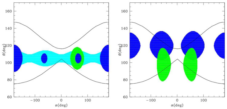
Very sophisticated U(θ, α) are included in the numerical FF derived by Bahar, Jernigan et al.[11, 12] and in the UNRES FF by Sheraga et al. [14, 16], which is analytical but involves a very large number of parameters. Here we analyze the FF with simpler analytical terms. Usually these include a quite accurate dihedral energy term U ^α, with terms in sin(nα) and cos(nα) with n up to 6 [3, 10], although it was shown that the terms in cos(α) and cos(3α) are the most relevant[8,9,13]. In fact, these were included also in the most recent versions of the Gō models[17]. Conversely, the bond angle term U(θ) is usually treated as harmonic. In order to include the dependence of the equilibrium θ on the secondary structure, different strategies have been adopted. An explicit correlation θ(α) was assumed by Levitt [3], that reduced the dimensionality of the α, θ plot to a line. More realistic α, θ plots can be obtained with an approach like that of Head-Gordon[8], that uses an accurate dihedral term depending on the aminoacid type, reproducing the pattern typical of the helices, sheets or turns depending on the aminoacid type (whose helix-sheet-turn propensity must be known a priori), while an harmonic bond angle term is used with an equilibrium θ₀ = 105deg that is an average of the typical helix and sheet value (see fig. 4, left). Alternatively, angle and dihedral energy terms typical for the β sheet were used, and additional terms depending on the second and third neighbour distance along the chain were used to tune the α-helix propensity, like in Mukherjee et al[13] (see fig. 4, right). As can be seen from the plots, these FFs may give a quite accurate pattern of the density plot (at least for the dihedral angle) for given secondary structures, but they are not very appropriate in describing situations when the propensity for a given secondary structure is not very well defined. For instance, they are inadequate to describe the α θ plot for glycine.

Figure 4.

Typical α, θ density maps for two different kinds of FF. Left: Head-Gordon-like FF; right: Mukherjee-like FF. Green=helix, blue=sheet, cyan=turn.

5 A new Force Field with an accurate bond angle interaction

We recently proposed a different approach[15] including an accurate bond angle term U^θ. We use a quartic double well potential for the bond angle potential

$$U^{\theta }=\frac{1}{2}{k}_{\alpha }{(\theta -{\theta }_{\alpha })}^2+\frac{1}{3}\mathit{\text{k}}\prime {(\theta -{\theta }_{\alpha })}^3+\frac{1}{4}\mathit{\text{k}}″{(\theta -{\theta }_{\alpha })}^4$$

where θ_α ≃ 90deg corresponds to the first minimum (typical of the alpha helix). The other parameters are related to the position of the second minimum θ_β, to the relative stability $\mathrm{\Delta }{U}^{\theta }=U_{\beta }^{\theta }-U_{\alpha }^{\theta }$ and to the (left and right) barriers $\mathrm{\Delta }{U}_{\alpha }^{\theta },\mathrm{\Delta }{U}_{\beta }^{\theta }$ via the following relations:

$$\begin{array}{l}\mathrm{\Delta }={\theta }_{\beta }-{\theta }_{\alpha }\mathit{\text{k}}\prime =-\frac{k_{\beta }+2k_{\alpha }}{\mathrm{\Delta }}\mathit{\text{k}}″=\frac{k_{\alpha }+k_{\beta }}{{\mathrm{\Delta }}^2}\\ \mathrm{\Delta }{U}^{\theta }=\frac{{\mathrm{\Delta }}^2}{12}(k_{\beta }-k_{\alpha })\mathrm{\Delta }{U}_{\alpha }^{\theta }=\frac{{\mathrm{\Delta }}^2}{12}\frac{k_{\alpha }^3}{{(k_{\alpha }+k_{\beta })}^3}(k_{\alpha }+2k_{\beta })\mathrm{\Delta }{U}_{\beta }^{\theta }=\frac{{\mathrm{\Delta }}^2}{12}\frac{k_{\beta }^3}{{(k_{\alpha }+k_{\beta })}^3}(k_{\beta }+2k_{\alpha })\end{array}$$

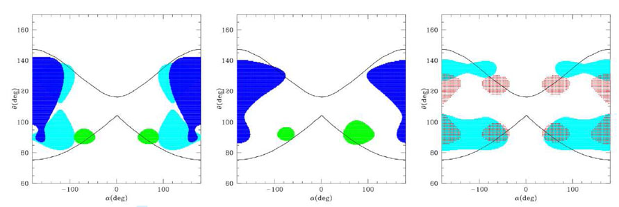
The dihedral term was taken as a harmonic (or harmonic cosine) with equilibrium value depending on the a priori known secondary structure. The (amino acid-dependent) parameters were derived through a statistical analysis of crystallographic structures, using the Boltzmann inversion[15]. The α, θ plots for helix-propense (green), sheet-propense (blue) and glycine-like amino acids are reported in fig. 5 (left). The accuracy of these maps is especially evident in the glycine-like pattern, where our force field reproduces the small separation between the helix-like and sheet-like regions, and in the sheet pattern (blue) where the peculiar shape with a small protuberance towards the θ = 90deg present in the “Generic” map of fig. 3 is reproduced. This FF has proven successful in reproducing the flap opening dynamics in the HIV-1 protease, which depends on a very peculiar motion of the glycine rich apt tips, and its dependence on the mutations in this region[15,22].

Figure 5.

α, θ density maps for the FF in the present work. Left: version with harmonic cosine dihedral potential; Center and right: version with cosine sum dihedral potential. Different maps are obtained giving different weights to the terms, in order to reproduce the map for sheet (blue), helix (green), glycine (cyan) and a generic model (red).

Here we propose a further improvement of the potential. We combine our double-well U^θ with a cosine-sum U^α similar to the potential of Head-Gordon et al[8]

$$U^{\alpha }=A(1+\text{cos}(\alpha ))+B(1+\text{cos}(3\alpha ))+C(1+\text{cos}(\alpha +\pi /4))+D(1+\text{cos}(2\alpha ))$$

whose terms have the following meaning. The first has a minimum at α = 180deg corresponding roughly to the sheet or extended structures. The second has additional minima at α = ±60deg, corresponding to helical structures. The third has a single minimum at α = 135deg and introduces an asymmetry that favors the right handed helices with respect to the left handed. The fourth has minima at α = ±90deg and can enforce the helix propensity. By giving different weights to the helix-like or sheet-like terms in U^α and U^θ and tuning the asymmetry term, one can reproduce quite realistic density plots. In fig. 5, center, density plots for helix-like (green) and for sheet-like (blue) structures are reported. In fig. 5, right, we report the density plot for glycine (cyan), obtained using approximately the same weight for the helix and sheet terms and no asymmetry. Finally, in red we report an hypothetical “generic” potential as simple as possible, including only the first and second terms in U^α. This does not resemble closely any of the “experimental” density plots, but contains all the secondary structures with approximately the same weight, including also the very uncommon polyproline helix (located at ~ 100, ~ 120) and its right handed counterpart.

6 Applications: α-helix to β-sheet transition in a minimal polypeptide model

We now illustrate the above concepts with a simple polypeptide model. We do not aim here to describe any specific poly-aminoacid type, an accurate amino acid type dependent parameterization will be the matter of a further paper. However this model could apply to a sheet-former, like poly-valine. In addition to the U^α and U^θ we used a Morse non-bonded interaction potential

$$U^{nb}=\in [{(1-\text{exp}(-\alpha (r-\sigma )))}^2-1]$$

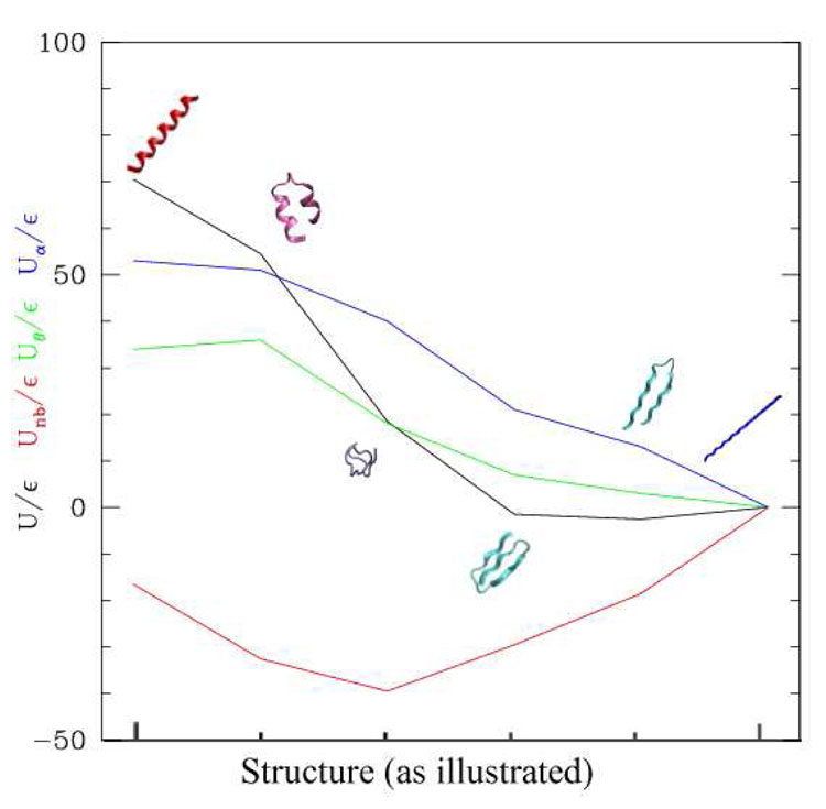
where σ = 6:1 Å is the bead diameter, α = 0:7 is the well width parameter and ∈ is taken as an energy unit. Since the helices, sheets and random coils are characterised by a different number of non-bonded contacts, the relative stability of the different secondary structures depends on a delicate balance between ∈ and ΔU^α;θ = ΔU^α + ΔU^θ. We chose the parameters in such a way that ΔU^α;θ = − 5∈ favours the sheet conformation. The energy barriers separating the helix from the sheet were set at $\mathrm{\Delta }{U}_{\alpha }^{\alpha }=6\in \text{and}\mathrm{\Delta }{U}_{\theta }^{\alpha }=7\in$ and a slight asymmetry towards the right handed helix was added to the dihedral potential (see fig. 6 for the values of the parameters). The Cα-Cα bonds were constrained at the value 3:79 Å. We performed two simulated annealing runs on a 20-mer, starting from the αhelical and from the extended configuration, respectively. The DL_POLY code was used[23] for the simulation. The results are reported in fig. 6–fig. 8.

Figure 6.

Relative stability and energy terms of the conformations explored during the simulations. Black: total potential energy, red = non bonded energy, green: bond angle energy, blue: dihedral energy. All energies are expressed in units of ∈. The extended conformation is taken as the zero-level. Parameters of the dihedral and bond angle terms: A = 2∈, B = 4∈, C = 0:5∈, D = 0, $\delta U_{\alpha }^{\theta }=7\in ,\delta U_{\alpha }^{\theta }=9\in$. Representative structures extracted from the simulations are reported: red=α-helix, pink=“broken-helix”, violet=random coil, cyan=β-hairpin and three-fold β-sheet.

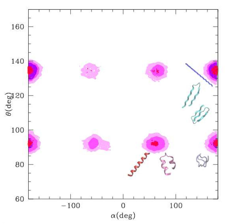
Figure 8.

α, θ plot evaluated along the trajectories of the two simulations. Violet: simulation starting from the extended conformation. Pink-magenta-red: simulation starting from the α helix at increasing density values. The representative structures of the populated regions are reported.

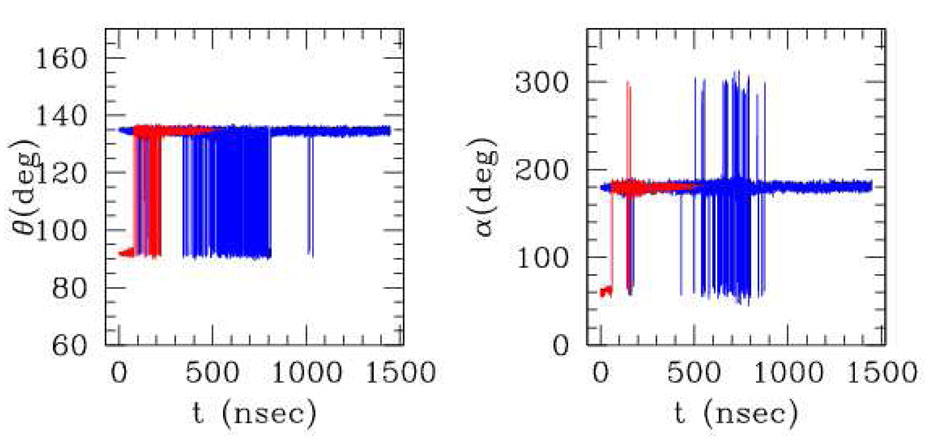
Fig. 7 reports the representative angles and dihedrals along the simulation. In the simulation starting from the α-helix (red) the transition to a globular random coil structure occurs after about 100 nsec at the temperature kT = 0:6∈, after passing through a metastable “broken helix” conformation (see fig6). As the temperature is raised up to kT =~ ∈, the system explores globular structures and finally, upon cooling down, it stabilizes in a three-fold β-sheet, i.e. a β-sheet with two β-turns located approximately at the 8th and 14th residue along the chain (see fig6). In the simulation starting from the extended structure (blue), the system tends to contract to a globule after about 100 nsec, then again stabilizes to a three-fold beta sheet. As the temperature is raised up to kT ≃ 2∈ (between 500 and 1000 nsec), the system melts into a globular state. During cooling down, it explores for long time intervals also the β-hairpin structures (β-sheets with one β-turn approximately in the middle of the chain), before definitely stabilizing in the three-fold β-sheet. Remarkably, the structures we find as (meta)stable states were also observed in simulations performed with more sophisticated models[24,25].

Figure 7.

“Representative values” of bond angles and dihedrals evaluated during the simulations starting from the α helix (red) and from the extended structure (blue). The “representative value” is evaluated as follows. For θ: for each timestep, all the 18 θ angles along the chain are measured, and two average values are calculated, one for the “extended” and one for the “helical” (conventionally separated by the value 113 deg). The representative value for θ is then chosen as the (average) value of the the most populated structure, for each timestep. For α: same procedure, except that in this case three separate average values are calculated for right handed (between 0 and 115 deg) or left handed helices (between −115 and 0) and for extended (otherwhise).

This dynamical behavior can be explained on the basis of the energy landscape of the system, reported in fig. 6. The energy terms combine in such a way that the helical structures are less stable while the sheet structures (both β-hairpin and three-fold β sheet) have a very similar energy and are slightly more stable than the extended one. The definitive choice for the three-fold β sheet may be due to the entropic factor.

The α, θ density plot for the two simulations is shown in fig. 8. The violet map is evaluated on the trajectory of the simulation starting from the extended conformation. Only the area corresponding to the βsheet and extended structures is populated, with a small population of the globular region located at α ≃ 180, θ ≃ 90. The map in red corresponds to the simulation starting from the αhelix. The transition to the βsheet passes through the molten globule region, however as can be seen from the maps obtained with lower levels of populations (magenta and pink), other region are also (slightly) populated. The pink map resembles the “generic” map (in red in fig. 5) although the effect of the asymmetry term that biases the system towards the “right handed” structures is evident.

7 Conclusions

In this paper we have reported two kinds of result. First we have derived analytical relationships to convert the internal backbone coordinates of the all-atoms representation of the polypeptide chain to the internal coordinates of the one(two) beads CG representation, namely the bond angles and dihedrals θ and α. This result has a general applicability to all cases where the geometry of the backbone must be described and only the coordinates of the Cαs are available, for instance with low resolution or CG models. We have used these relationships to convert the Ramachandran plot into new two-dimensional density plots in terms of the backbone variables θ, α. These α, θ density plots can be used as the Ramachandran plot, i.e. to test the reliability of proteins models, in low resolution or CG models, when the original Ramachandran plot cannot be used.

Second, we have illustrated these ideas on a minimal one-bead polypeptide model that accounts for the transition from αhelices to β sheets. With respect to the models available in the literature, our model contains a more sophisticated bond angle term, that allows one to reproduce quite accurately the α, θ plot. Furthermore, in spite of its simplicity, this model is shown to explore the conformational space as accurately as more sophisticated multiple beads models. It is arguable that an optimization and fine tuning of the parameters of the model can account for the helix or sheet propensities of the different amino-acids and reproduce more complex structures and transitions.

Supplementary Material

File001. Supporting Information Available.

Supporting Information includes the derivation of the exact formula for the dihedral α as a function of ϕ, ψ This information is available free of charge via the Internet at http://pubs.acs.org.

References

- 1.Head-Gordon T, Brown S. Curr Opin Struct Biol. 2005;13:160–167. doi: 10.1016/s0959-440x(03)00030-7. [DOI] [PubMed] [Google Scholar]
- 2.Tozzini V. Curr Opin Struct Biol. 2005;15:144–150. doi: 10.1016/j.sbi.2005.02.005. [DOI] [PubMed] [Google Scholar]
- 3.Levitt M. J. Mol. Biol. 1976;12:59–107. doi: 10.1016/0022-2836(76)90004-8. [DOI] [PubMed] [Google Scholar]
- 4.Ueeda Y, Taketomi H, Gō N. Biopolymers. 1978;17:1531–1548. [Google Scholar]
- 5.Nguyen HD, Hall CK. Proc Natl Acad Sci USA. 2004;101:16180–18185. doi: 10.1073/pnas.0407273101. [DOI] [PMC free article] [PubMed] [Google Scholar]
- 6.Fujisuka Y, Takada S, Luthey-Schulten ZA, Wolynes PG. Proteins. 2004;54:88–103. doi: 10.1002/prot.10429. [DOI] [PubMed] [Google Scholar]
- 7.Favrin G, Irbäck A, Wallin S. Proteins. 2002;47:99–105. doi: 10.1002/prot.10072. [DOI] [PubMed] [Google Scholar]
- 8.Brown S, Fawzi NJ, Head-Gordon T. Proc Natl Acad Sci USA. 2003;100:10712–10717. doi: 10.1073/pnas.1931882100. [DOI] [PMC free article] [PubMed] [Google Scholar]
- 9.Friedel M, Shea J-E. J Chem Phys. 2004;120:5809–5823. doi: 10.1063/1.1649934. [DOI] [PubMed] [Google Scholar]
- 10.McCammon JA, Northrup SH, Karplus M, Levy RM. Biopolymers. 1980;19:2033–2045. [Google Scholar]
- 11.Keskin O, Bahar I. Fold Des. 1998;3:469–479. doi: 10.1016/S1359-0278(98)00064-9. [DOI] [PubMed] [Google Scholar]
- 12.Bahar I, Jernigan RL. J Mol Biol. 1997;166:195–214. doi: 10.1006/jmbi.1996.0758. [DOI] [PubMed] [Google Scholar]
- 13.Mukherjee A, Bagchi B. J Chem Phys. 2004;120:1602–1612. doi: 10.1063/1.1633253. [DOI] [PubMed] [Google Scholar]
- 14.Pillardi J, Czaplewski C, Liwo A, Lee J, Ripoll DR, Kazmierkiewicz R, Oldziej S, Vedemeyer WJ, Gibson KD, Arnautova YA, Saunders J, Ye Y-J, Sheraga HA. Proc Natl Acad Sci USA. 2001;98:2329–2333. doi: 10.1073/pnas.041609598. [DOI] [PMC free article] [PubMed] [Google Scholar]
- 15.Tozzini V, McCammon JA. Chem Phys Lett. 2005;413:123–128. [Google Scholar]
- 16.Zacharias M. Protein Sci. 2003;12:1271–1282. doi: 10.1110/ps.0239303. [DOI] [PMC free article] [PubMed] [Google Scholar]
- 17.Koga N, Takada S. J Mol Biol. 2001;313:171–180. doi: 10.1006/jmbi.2001.5037. [DOI] [PubMed] [Google Scholar]
- 18. http://pdbbeta.rcsb.org/pdb/
- 19.Mathews CK, van Holde KE, Ahern KG. Biochemistry. Benjamin Cummings Serie: Addison Wesley Longman inc eds; 2000. [Google Scholar]
- 20.Voet D, Voet JG. Biochimica. Zanichelli: 1997. [Google Scholar]
- 21.Reith D, Pütz M, Müller-Plate F. J Comp Chem. 2003;24:1624–1636. doi: 10.1002/jcc.10307. [DOI] [PubMed] [Google Scholar]
- 22.Chang C-E, Shen T, Trylska J, Tozzini V, McCammon JA. Biophys J. in press. [Google Scholar]
- 23.Smith W, Forester TR. J. Molec. Graphics. 1996;14:136. doi: 10.1016/s0263-7855(96)00043-4. [DOI] [PubMed] [Google Scholar]; Smith W, Yong CM, Rodger PM. Molecular Simulation. 2002;28:385. [Google Scholar]
- 24.Ding F, Borreguero JM, Buldyrey SV, Stanley HE, Dokholyan NV. Proteins. 2003;53:220–228. doi: 10.1002/prot.10468. [DOI] [PubMed] [Google Scholar]
- 25.Nguyen HD, Marchut AJ, Hall CK. Protein Sci. 2004;13:2909–2924. doi: 10.1110/ps.04701304. [DOI] [PMC free article] [PubMed] [Google Scholar]
Associated Data
This section collects any data citations, data availability statements, or supplementary materials included in this article.
Supplementary Materials