Effects of Temperature and Salt Concentration on the Structural Stability of Human Lymphotactin: Insights from Molecular Simulations

Abstract

Extensive molecular dynamics (MD) simulations (∼ 70 ns total) with explicit solvent molecules and salt ions are carried out to probe the effects of temperature and salt concentration on the structural stability of the human Lymphotactin (hLtn). The distribution of ions near the protein surface and the stability of various structural motifs are observed to exhibit interesting dependence on the local sequence and structure. Whereas chloride association to the protein is overall enhanced as the temperature increases, the sodium distribution in the C-terminal helical region and, to a smaller degree, the chloride distribution in the same region are found higher at the lower temperature. The similar trend is also observed in non-linear Poisson-Boltzmann calculations with a temperature-dependent water dielectric constant, once conformational averaging over a series of MD snapshots is done. The unexpected temperature dependence in the ion distribution is explained based on the cancellation of association entropy for ion-sidechain pairs of opposite-charge and like-charge characters, which have positive and negative contributions, respectively. The C-terminal helix is observed to partially melt while a short • strand forms at the higher temperature with little salt dependence. The N-termal region, by contrast, develops partial helical structure at a higher salt concentration. These observed behaviors are consistent with solvent and salt screening playing an important role in stabilizing the canonical chemokine fold of hLtn.

I. INTRODUCTION

For cells to function normally, the activities of cellular components need to be strictly regulated.¹ For proteins, an important regulatory mechanism involves conformational transitions induced by a chemical modification.^2–5 Alternatively, many proteins are regulated through non-covalent but direct interactions with other small molecules or biomolecules.^6,7 It has been long recognized, however, that the structure and therefore function of biomolecules can also be regulated by non-specific interactions, such as changes in the local osmolyte/salt concentration;^8,9 these changes can be induced by either a global change in the cellular environment or, more intriguingly, the activity of other nearby biomolecules.¹⁰ Evidently, understanding the effect of ions, or small solutes in general, on the structure and stability of biomolecules is an important step towards elucidating the function of biomolecules in the realistic cellular environment.¹¹

The influence of salt concentration on the stability of polyelectrolytes, such as DNA and RNA molecules, has been analyzed by many previous experimental and theoretical studies,^12–18 though there are still issues remain to be resolved.^19–21 For protein systems, the effects of various salts and other small molecules, e.g., the ”salting in” and ”salting out” effects associated with the Hofmeister series,^9,22–26 have been documented in great detail, although a unifying theory that can quantitatively predict the effect of salt concentration on the stability of protein is not yet available.^27–32 The importance of salt on protein stability was also illustrated in several molecular dynamics simulations.^33,34 Although including counter ions for proteins with a low overall charge was shown not as important,³⁵ proteins with a higher overall charge are more sensitive to the ionic environment. For the highly charged βARK PH domain (+6 overall charge), for example, including ions to near physiological concentration was found necessary to stabilize the protein during simulation since otherwise there were not enough ions near the protein surface to screen the strong interactions among charged residues.³³.

Most previous studies of salt and small solute effects focused on the process of folding/unfolding between the native and denatured states. Depending on whether the solute preferentially partitions close to or away from the biomolecular surface, different states are favored by different small solutes.^9,24 There are, however, interesting cases in which multiple distinct folded states co-exist and the equilibria among them are perturbed by non-specific variables such as temperature and salt concentration.^36,37 In this context, human lymphotactin (hLtn) is a remarkable example. Lymphotactin belongs to the chemokine group^38–40 that is regulated by proinflammatory or infectious stimuli, and was shown to be expressed mainly in activated T and Natural Killer (NK) cells.^41,42 The human Lymphotactin is implicated in allograft rejection, inflammatory bowel diseases and other immune system related diseases.⁴³ In general, chemokines stimulate cells of the immune system through activating specific G protein-coupled receptors (GPCRs).⁴⁴ In addition, they aid in the recruitment of leukocytes by binding to cell surface glycosaminoglycans (GAG),⁴⁵ which are highly sul-fated oligosaccharide components of the extracellular matrix. Therefore, each chemokine must display two high affnity binding surfaces, and some chemokines dimerize to create a bifunctional species that can satisfy both functionally important interactions.

Specifically for hLtn, two distinct folds were detected by NMR to equally populate under the physiological condition (37 °C, 154 mM salt), although the specific function of each fold is still under active research.³⁶ The canonical chemokine fold consists of a flexible N-terminal tail, a three strand β-sheet and an α-helix at the C-terminus (Fig.1); this fold was observed to be particularly stable under the condition of high salt concentration (200 mM NaCl) and low temperature (10 °C).³⁶ Under the condition of no salt and high temperature (45 °C), however, NOE data³⁶ suggested a non-chemokine fold in which the C-terminal α-helix became unraveled and the β-sheet was reordered with the addition of a ‘β0’ strand. Remarkably, the rearrangement of secondary structural element involves the disruption of nearly every backbone hydrogen bond and formation of new bonds between a completely different sets of donor-acceptor pairs. To further complicate the analysis, this fold was observed to have the propensity to dimerize under the same condition. Although useful for secondary structural analysis, the NOE data were insufficient to determine a complete structure for the non-chemokine fold until very recently (B. Volkman, private communication).

FIG. 1.

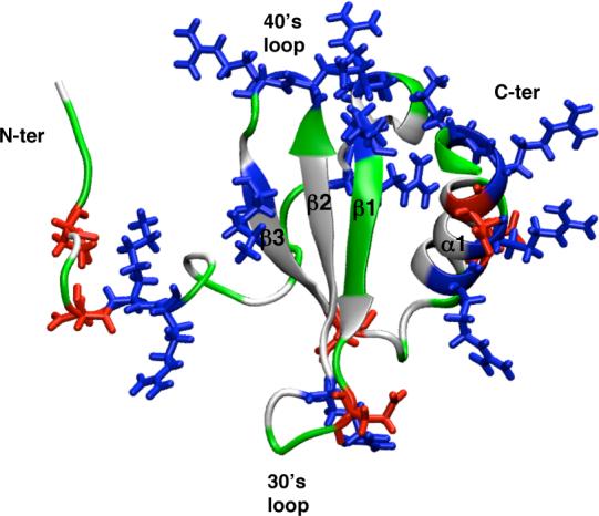
The structure and location of charged residues (shown in line form) in the canonical chemokine fold of hLtn (averaged NMR structure from PDB code 1J9O). The residues are colored based on the residue type: white for non-polar, green for polar, red for negatively charged and blue for positively charged residues.

In these NMR studies,³⁶ temperature and salt concentration were changed simultaneously, therefore it was not possible to understand the impact of each variable on the equilibrium between the two hLtn folded conformations. In addition, it is possible that the two variables are not independent of each other; e.g., temperature may further perturb the structure of hLtn indirectly by influencing the distribution of salt ions around the protein.

The spectacular conformational changes in hLtn makes it an attractive system for further exploring the role of salt on protein structure and stability. Towards this end, we study the behavior of hLtn under different salt concentrations using molecular dynamics simulations. Considering the non-specific nature of protein-salt interactions, molecular dynamics simulations are useful because they are capable of providing a microscopic mechanistic picture for salt binding to proteins and for how such interactions may influence the structural properties of proteins.^27,28 Simulations with different combinations of salt concentration and temperature are carried out, which further allow us to probe whether the salt effects are perturbed significantly by temperature. To the best of our knowledge, although the effect of salt on protein conformation has been studied rather extensively,^{27,28,33–35} the combined effects of temperature and salt concentration on protein stability has not been systematically investigated using molecular simulations. The current ten-nanosecond-scale simulations reveal that the distribution of salt ions around the protein surface can be rather sensitive to temperature; more interestingly, the trend in the temperature dependence may depend on the local sequence and structure of the protein.

II. COMPUTATIONAL METHODS

Since only the chemokine-fold structure of hLtn has been solved using NMR,³⁶ only this conformation is studied using molecular dynamics simulations. Different combinations of temperature and salt concentration are used to produce totally about 70 ns of MD trajectories. With these ten-nanosecond-scale simulations, the major motivation is to observe the initial structural responses in hLtn to changes in each environmental variable or with variations in both. Although only limited structural changes compared to those revealed by the NOE data³⁶ are observed in the 70 ns trajectories, the distribution of ions at the protein surface is noticeably affected by temperature changes. For comparison, non-linear Poisson-Boltzmann calculations^46,47 are also carried out to examine the effect of temperature on the salt distribution around hLtn.

A. Explicit Solvent Molecular Dynamics

Although salt-dependence can be included in molecular dynamics simulations using implicit solvent models through, for example, Debye-Hückle theory,^48,49 many previous studies highlighted the role of specific ion-binding sites, which can not be described with a mean- field approach.^50,51 For example, for the binding of guanosine-3’-monophosphate (3’GMP) to ribonuclease Sa (RNase Sa), the experimental findings regarding the salt and temperature dependence were opposite to the prediction from Poisson-Boltzmann calculations.⁵⁰ Therefore, explicit solvent and salt simulations are carried out here using the periodic boundary condition.⁵²

1. Simulation set-up

As summarized in Table I, four simulations are performed with different combinations of salt concentration and temperature to probe the collective and individual effects of these conditions on the structural stability of hLtn. The starting structure in all MD simulations is the averaged NMR structure (PDB code 1J9O⁵³) for the ‘canonical’ chemokine-fold, which was obtained under the condition of 10 °C and 200 mM NaCl concentration. The disordered C-terminal residues (69 to 93) are removed from the structure for simulation in order to minimize the size of the periodic boundary box. This simplification is justified by the experimental observation³⁶ that truncation of this region did not alter the environment-dependent conformational transition in the rest of the protein; this random coil, however, is necessary for the function of hLtn in signaling of intracellular calcium mobilization⁵⁴ and as a lymphocyte chemoattractant.⁵⁵

TABLE I.

Simulation conditions for the molecular dynamics study of hLtn

Statea	Number of Cl− ions	Number of Na+ ions	Average Box Length (Å)	Comments
s10	7	0	61.4	Stable Chemokine-fold Condition
n45	7	0	62.0	Non-chemokine Conformation Condition
n10	32	25	62.0	Perturbationb of Salt Concentration Only
s45	32	25	62.6	Perturbationb of Temperature Only

^aThe notations are: `n' for [NaCl]=0 mM, `s' for [NaCl]=200 mM, `10' for T=10 °C and `45' for T=45 °C.

^bRelative to the stable chemokine-fold condition

The protein is initially solvated with the Solvate program by Grubmüller⁵⁶, using 0 or ∼200 mM concentration. Additional ions are added by replacing randomly selected water molecules, up to the numbers summarized in Table I, to ensure charge neutrality of the simulation system.

The molecular dynamics simulations are carried out using the program package CHARMM⁵⁷, with the CHARMM22 force field for proteins⁵⁸ and a modified⁵⁹ TIP3P model for water.⁶⁰ The SHAKE algorithm⁶¹ is used to constrain all the bonds involving hydrogen atoms to allow a time step of 2 fs with the leap-frog integration scheme.⁵² A switching scheme⁶² for interatomic distances between 10 and 12 Å is used for van der Waals interactions. For electrostatic interactions, the Ewald summation⁶³ approach is employed with parameters optimized following the discussion of Feller et al.⁶⁴ Specifically, the Particle Mesh Ewald (PME) scheme^65,66 is used with a Gaussian width of 0.3Å. The real-space interactions are calculated with a cutoff at 12 Å and a shifting function between 10 and 12 Å; the reciprocal-space contributions are calculated with the Fast Fourier Transform algorithm using 64 grid points per box length and an eighth order B-spline interpolation scheme. No correction term⁶⁷ is needed since the net charge of all simulated systems was zero.

After the system is equilibrated using NVE simulations and gradually decreasing harmonic constraints on the protein for ∼50 ps, production runs are performed with constant temperature and pressure. The temperature is constrained using the Nosé-Hoover algorithm^68,69 with a mass of 250 amu for the thermostat and a Hoover reference temperature that equals to the desired system temperature. The pressure is controlled with the Andersen algorithm⁷⁰ using a mass of 500 amu for the pressure piston, a reference pressure of 1 atm, a Langevin piston collision frequency of 10 ps⁻¹ and a Langevin piston bath temperature that equals to the desired system temperature. The s10 and n45 simulations are carried out for 20 ns, and the n10 and s45 simulations are carried out for 14 ns.

2. Analysis of results

To characterize the structural properties of hLtn under different conditions, standard analyses are carried out using the MD trajectories; the simulation data are sampled at 1 ps intervals, thus 14,000 configurations for n10 and s45 and 20,000 configurations for s10 and n45 are used. These analyses include the calculation of the root-mean-square-deviation (RMSD) relative to the average NMR structure, atomic root-mean-square-fluctuations (RMSF), order parameters for the main chain NH bonds⁷¹ (see Supporting Materials) and secondary structural element analysis. For the secondary structure analysis, the STRIDE algorithms⁷² implemented in VMD⁷³ are used.

To characterize the distribution of ions around the protein, several types of measurement are made. Although no Na⁺ is included in the n10/n45 simulations, Cl⁻ ions are added (see Table 1) for the purpose of neutralizing the total charge of the system in these simulations; therefore, ion distributions are calculated for Cl⁻ in all simulations while those for Na⁺ are only calculated for the s10/s45 simulations. First, the radial distribution functions of Cl⁻ and Na⁺ relative to the protein surface, $g_{surf}^{C{l}^{-}∕N{a}^{+}}\left(r\right)$, are calculated. The shortest distances between a specific type of ions to the protein atoms are collected and binned ($\delta N_{surf}^{C{l}^{-}∕N{a}^{+}}\left(r\right)$). The volume factor (δV ) corresponding to the bin (r, dr) is estimated using the volume function in CHARMM (COOR VOLU) with all protein atoms (irrespective of atom type) having a radius of either r+dr/2 or r-dr/2; i.e., δV = V (r+dr/2)-V (r-dr/2). The ion-surface radial distribution function is then calculated as,

$$g_{surf}^{C{l}^{-}∕N{a}^{+}}\left(r\right)={\rho }_{\infty }^{C{l}^{-}∕N{a}^{+}}\frac{\delta N_{surf}^{C{l}^{-}∕N{a}^{+}}\left(r\right)}{\delta V}$$ (1)

in which the ‘bulk number density’ (${\rho }_{\infty }^{C{l}^{-}∕N{a}^{+}}$) is estimated by dividing the number of ions by the average volume of the simulation box. Since different simulations apparently have different bulk ion densities, the radial distribution functions are also integrated over the distance from the protein surface ($N_{surf}^{C{l}^{-}∕N{a}^{+}}\left(r\right)$) to provide a more explicit description for the average number of ions accumulated around the protein. We note that it might be more physical to take the van der Waals radii of the protein atoms into account when measuring the ion-protein-surface distances, although this complicates the volume calculations and therefore is not pursued. Even with the current definition of ion-protein distances, the volume estimate is somewhat problematic for short distances because cavities in the protein (where ions are never found) are not excluded. These subtleties, however, are not expected to change the qualitative picture for ion distributions around the protein.

To gain further insights into the location of ion accumulations, radial distribution functions are also calculated for ion-charged-sidechain ($g_{chrg}^{C{l}^{-}∕N{a}^{+}}\left(r\right)$), ion-polar-sidechain ($g_{pol}^{C{l}^{-}∕N{a}^{+}}\left(r\right)$) and ion-backbone ($g_{bb}^{C{l}^{-}∕N{a}^{+}}\left(r\right)$) pairs. For the calculation of $g_{chrg}^{C{l}^{-}∕N{a}^{+}}\left(r\right)$, the shortest distance between the ion and the heavy atom(s) in the charged group (NH₁ & NH₂ for Arg, N_ζ for Lys, O_†'s for Asp and O_ε's for Glu) is used. For $g_{pol}^{C{l}^{-}∕N{a}^{+}}\left(r\right)$, the protein atoms considered include O_γ for Ser, O_γ1 for Thr, O_η for Tyr, N_ε1 for Trp, N_δ2 and O_†1 Asn, and N_ε2 and O_ε1 for Gln. For $g_{bb}^{C{l}^{-}∕N{a}^{+}}\left(r\right)$, the amide N and carbonyl O is considered as the partner for Cl⁻ and Na⁺, respectively. Integrations approximately over the first ($N_{chrg∕pol∕bb}^{C{l}^{-}∕N{a}^{+}}\left(r_1\right)$) and second ($\Delta N_{chrg∕pol∕bb}^{C{l}^{-}∕N{a}^{+}}(r_2;r_1)=N_{chrg∕pol∕bb}^{C{l}^{-}∕N{a}^{+}}\left(r_2\right)-N_{chrg∕pol∕bb}^{C{l}^{-}∕N{a}^{+}}\left(r_1\right)$) peaks in the corresponding radial distribution functions are also carried out to give the average number of ions around specific regions near the protein; it is important to look at both peaks because the solvent separated binding is commonly observed for interactions involving ions.

B. Non-linear Poisson-Boltzmann (PB) calculations

To compare with explicit solvent and ion simulations, non-linear Poisson-Boltzmann calculations⁴⁶ are also carried out; the linearized version is also tested and the result is very similar because the salt concentration of interest is low and only mono-valent ions are involved. It's particularly interesting to investigate if the PB approach captures the similar temperature effect on the salt distribution around the protein. The PB calculations are carried out for 200 snapshots collected from each of the explicit solvent-salt MD trajectories (s10 and s45). The set of atomic radii established by Roux and co-workers⁷⁴ is used together with a solvent probe radius of 1.4 Å and a stern ion-exclusion layer of 2 Å. The partial charges are those in the standard CHARMM 22 force field for proteins.⁵⁸. The grid consists of 251³ points spaced by 0.5 Å, which is found sufficiently fine for studying the ion distribution around the protein. As to the value of the dielectric constant, a value of 2 is used for the protein and assumed to be independent of temperature. The dielectric constant of bulk water, however, is taken as a function inversely dependent on the temperature;⁷⁵ specifically, the value is 83.9 and 71.6 at 10°C and 45°C, respectively. For comparison, calculations are also carried out with a fixed water dielectric constant of 83.9 at different temperatures.

Once the electrostatic potentials (ϕ(r)) are solved using PB, the ion distribution can be obtained by the Debye-Hückle expression,⁴⁸

$${\rho }_{N{a}^{+}∕C{l}^{-}}\left(\mathbf{r}\right)={\rho }_{\infty }exp[-\beta q_{N{a}^{+}∕C{l}^{-}}\varphi \left(\mathbf{r}\right)]$$ (2)

where ρ_∞ is the bulk salt concentration, β the inverse temperature and q the charge of a specific type of ion.

III. RESULTS

In this section, we first describe the structural stability of hLtn in the chemokine-fold under different conditions (combinations of salt concentration and temperature) as observed from multiple 10-nanosecond-scale molecular dynamics simulations. We then analyze, in detail, the distribution of salt ions around the protein based on these explicit solvent simulations; the results are also compared to those from Poisson-Boltzmann calculations for snapshots collected from the MD trajectories.

A. Structural Stability

The N-terminus of hLtn contains a disordered region, which is known as an important part of the dimerization interface for some CC type chemokines^76–79 and possibly for, along with the 30's loop, binding to the XCR1 receptor.⁸⁰ The specific function of this region in hLtn, however, remains to be clarified. Due to its disordered nature, this region samples a wide range of conformations that wildly differ from the averaged NMR structure in all simulations (Fig.2). As a result, the RMSD for the entire protein as compared to the average NMR structure was very large (∼ 8 Å) in all simulations; without the contribution from the first twenty residues, however, the RMSD was below 4 Å under all four conditions (see Supporting Materials).

FIG. 2.

Final snapshots from the molecular dynamics simulations of hLtn, in yellow, under the four simulation conditions (see Table I for details). Each snapshot is RMS best-fitted to and superimposed with the average NMR structure (PDB code 1j9o⁵³), depicted in blue. Figures are produced by VMD⁷³.

In the chemokine-fold, the C-terminus of hLtn consists of an α-helix spanning 13 residues (Thr 54-Lys 66, see Fig.1).⁵³ The stability of this C-terminal helix is observed in the current simulations to depend on the temperature but much less sensitive to the salt concentration. For example, the last snapshot in each simulation (Fig.2) showed that this helix unraveled to a greater extend in the n45/s45 simulations than in the n10/s10 sets. When the RMSD is calculated without contributions from the last 5 residues, the decrease is more significant for the 45 °C simulations (see Supporting Materials). The plot of the secondary structure as a function of simulation time (Fig.3) further demonstrates the greater unraveling of the C-terminal helix at the high temperature.

FIG. 3.

Secondary structures of hLtn during the four MD simulations under different conditions (see Table I for details). The color coding is: green for β strand, magenta for α helix, red for π-helix, white for turn and for coil. These plots are produced by VMD⁷³ using the STRIDE algorithm for secondary structure determination⁷².

The secondary structure plot also reveals the intermittent formation of new structural motifs near the N-terminus, namely an α-helix involving the first 8 residues and a small β-strand involving residues Ser 13 and Leu 14. The new β-strand is close to Cys 11, which forms the sole disulfide bridge to Cys 48 on the β3 sheet. It is evident from Fig.3 that formation of the new β strand is more frequent for both high-temperature simulations, which is consistent with the idea that β sheets are stabilized at higher temperatures due to the temperature dependence of hydrophobic interactions.⁸¹ Although this new β-strand occurs at the same location as the β0 proposed for the non-chemokine fold, the conformational changes seen in the MD simulations are different from the much more dramatic structural changes inferred from the NOE data under the n45 condition.³⁶ The NOE data are consistent with the three-strand β sheet undergoing a spectacular rearrangement by flipping β1 and β3 by 180 ° along the strand axis and a shifting of residue-residue contacts in the sheet, accompanied by the formation of a fourth β0 strand of 4 residues (Cys 11-Leu 14). It is unlikely that such dramatic changes can be seen in nano-second MD simulations, although the observed conformational changes might be the initial events that eventually lead to the larger scale reorganizations.

The other new structural motif, the N-terminus α-helix, is observed in both high-salt simulations, although the helix is more persistent (Fig.3) and visible (e.g., in Fig.2) in the s45 set. The formation of this helix was not seen in the NMR experiments, which sampled only the s10 and n45 conditions.³⁶.

For the rest of the protein, which contains the 3-strand β sheet and two loop regions (30's and 40's loops), the variations from the average NMR structure and among different simulations are much smaller. The 30's loop (Glu 31- Arg 35) exhibits larger mobility than the 40's loop (Lys 42- Leu45) at most conditions, as reflected by the substantially lower N-H order parameters for the 30's loop residues (see Supporting Materials). Interestingly, the 40's loop is found more mobile in only the s10 simulation, in which the backbone hydrogen bond between Leu 45 and Thr 41 is observed to break (see Supporting Materials). In the s45 simulation, two backbone hydrogen bonds close to the 30's loop is observed to break, which leads to the large fluctuations for Ile 29-Glu 31 than other simulations. It is logical to question whether these observations in high-salt simulations are related to the salt ion distribution in the 30's and 40's loop regions (see below).

B. Distribution of Ions

As discussed in many previous studies,^9,24,27,28 the role of ions in protein (and nucleic acids) stability can range from being non-specific, as in screening electrostatic interactions between charged or polar groups, to being highly specific, where the ion-site interaction contributes significantly to the local structural features. Therefore, it is important to determine the distribution of ions around the protein and establish whether the distribution is affected significantly by temperature.

1. Explicit solvent simulations

Chloride ions

As shown by the $N_{surf}^{C{l}^{-}}\left(r\right)$ plots in Fig.4a, there are clear accumulations of Cl⁻ on the hLtn surface. At a given salt concentration, the temperature dependence is clearly visible. Based on $N_{surf}^{C{l}^{-}}\left(r\right)$'s shown in Fig.4b, there is, on average, additional 0.5 Cl⁻ ion within 6 Å from the protein at 45 °C relative to 10 °C. Examination of integrated radial distribution functions for Cl⁻ around different protein groups offer further insights into the location that Cl⁻ ions accumulate and the corresponding temperature dependence. For example, $N_{bb}^{C{l}^{-}}\left(4.0\mathrm{Å}\right)$ clearly shows that Cl⁻ ions do not bind directly to the backbone atoms (Fig.5a), even in disordered regions of hLtn. In the 40's loop region, however, outer-sphere Cl⁻ binding to protein backbone is observed in both 45°C simulations, although the degree of accumulation is clearly higher at the high salt concentration, as reflected by the quantity $\Delta N_{bb}^{C{l}^{-}}(6.0\mathrm{Å};4.0\mathrm{Å})$ (Fig.5b). As expected, more Cl⁻ accumulations are observed around positively charged sidechains; as shown in Fig.5c,d, both inner- and outer-sphere interactions are prevalent. Two arginine residues specifically involved in GAG binding⁸², Arg 23 and Arg 43, are observed to coordinate with Cl⁻ ions (Fig.7a,b) and the association is particularly more notable in the s45 simulation. Even for other sites where binding is less pronounced, the high-temperature simulations consistently show a higher degree of Cl⁻ accumulation, regardless of the salt concentration. The interesting exception is observed at the C-terminal region (close to Asn 68), where the s10 simulation shows a somewhat higher degree of Cl⁻ binding, especially through solvent (Fig.5d), than the s45 simulation. Regarding the interaction with the polar but neutral sidechains, distinct peaks for $N_{pol}^{C{l}^{-}}$ in the 40's loop region are found, especially at the high temperature (Fig.5e); second-sphere coordinations are less pronounced and appear less specific (Fig.5f).

FIG. 4.

Ion distribution around the protein surface in different simulations (see Table I). (a-b): Integrated radial distribution function, $N_{surf}^{C{l}^{-}∕N{a}^{+}}\left(r\right)$, of ions from the nearest atom at the hLtn surface. (c-f): Three dimensional ion distribution averaged over the entire course of the explicit solvent-ion simulations, pictured with the final snapshot for each simulation condition. The ion distributions are calculated using Surfnet⁹⁹, with a contour level of 1.5 ions per nm³. Positively charged sidechains (Arg and Lys) are colored blue and negatively charged sidechains (Asp, Glu) are colored red. Chloride contours are colored green and sodium contours are colored orange. These pictures are made with the program InsightII.

FIG. 5.

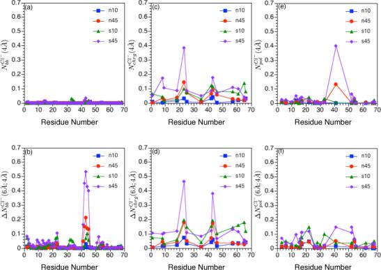
Integrated ion-site radial distribution functions for Cl⁻ ions relative to charged residues, polar residues and backbone atoms of hLtn under different simulation conditions (see Table I). Approximate (a) first and (b) second peak integration for Cl⁻ around backbone nitrogen atoms; (c)-(d): the same set for Cl⁻ around terminal atoms of positively charged residues (N_η1 and N_η2 for Arg and N_ζ for Lys); (e)-(f): the same set for Cl⁻ around atoms in the polar sidechains. The integration limits are taken to be 4 Å and 6 Å because they are the approximate locations for the first and second minima in the Cl⁻ radial distribution functions around different protein sites. See Computational Methods for protein atoms used in the analysis; note that for (c) and (d), the backbone nitrogen of the positively charged amino end group is used for Val 1.

FIG. 7.

Snapshots that illustrate the various binding modes for ion-protein interactions observed in different simulations. Chloride and sodium are colored green and orange, respectively; carbon is light blue, oxygen is red, nitrogen is dark blue and hydrogen is white, for which only the polar hydrogens are shown. (a) and (b) display the same snapshot from the end of the s45 simulation around the 40's loop. Residues Arg 23, Thr 41 and Arg 43 are represented by all atoms while only the backbone atoms are shown for Lys 42, Gly 44, Leu 45 and Lys 46. (c) and (d) display two separate snapshots of the s10 simulation at 8.66 and 14.47 ns into the simulation, respectively. The labeled residues display all the atoms, except Met 65 for which only the backbone atoms are shown in (c).

Sodium ions

Sodium ions associate more strongly with water than chloride ions.^22,25 As a result of the larger desolvation penalty, Na⁺ displays preferential exclusion from the protein surface compared to Cl⁻, as observed in previous simulations of small peptides^27,28. This trend is also observed here for hLtn. As shown in Fig.6, the degree of Na⁺ binding to protein backbone and (negative) charged residues is substantially lower compared to Cl⁻ accumulation; this is true for both inner- and outer-sphere interactions. The striking exception is observed at the C-terminal region at the lower temperature (s10 simulation), where significant Na⁺ accumulation is seen with both backbone (Fig.6a,b), the Asp 64 sidechain and the C-terminal carboxylate (Fig.6c,d); an example of binding is shown in Fig.7c. There is a notable peak in $\Delta N_{pol}^{N{a}^{+}}(5\mathrm{Å};3\mathrm{Å})$ near the 30's loop region at the low-temperature condition (Fig.6f), which is largely due to the second-sphere interaction between Tyr 27 with sodium ions that are bound to Asp 64 (Fig.7d). Nevertheless, the total average number of Na⁺ ions within 6 Å from the protein surface is substantially lower (by ∼ 3) than that of Cl⁻, regardless of the temperature. In other words, sodium ions are overall preferentially partitioned to the bulk compared to the chloride, although the C-terminal region of hLtn contains specific sites where Na⁺ preferentially binds at the lower temperature.

FIG. 6.

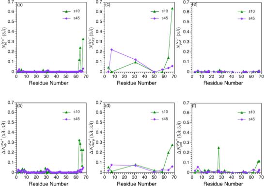
Integrated ion-site radial distribution functions for Na⁺ ions relative to charged residues, polar residues and backbone atoms of hLtn at different simulation conditions (see Table I). (a) First and (b) second peak integration for Na⁺ around backbone carbonyl oxygen atoms; (c)-(d): the same set for Na⁺ around terminal atoms of negatively charged residues (O_δ1 and O_δ2 for Asp and O_ε1 and O_ε for Glu); (e)-(f): the same set for Na⁺ around atoms in the polar sidechains. The integration limits are taken to be 3 Å and 5 Å because they are the approximate locations for the first and second minima in the Na⁺ radial distribution functions around different protein sites. See Computational Methods for protein atoms used in the analysis; note that for (c) and (d), both oxygens of the negatively charged carboxyl end group are used for Asn 68.

To summarize the overall findings regarding ion binding and the temperature dependence, the three-dimensional ion distributions averaged over the different trajectories are shown in Fig.4(c-f); the final structures from the corresponding trajectories are also shown to facilitate the visualization of ion distribution relative to the protein, although it should be understood that the protein structure, especially the N-terminal region, fluctuate significantly during the MD. A general increase of chloride density is observed at the higher temperature by comparing the n45 and n10 simulations, though the most noticeable area of increase concerns the 40's loop, which is also the pocket that contains a large number of positively charged sidechains (e.g., Arg 18, 23, 43 and Lys 25, 42, see Fig.1). The same trend is not as apparent for the s10/s45 sets, except for the enhanced accumulation around the 30's loop. For the sodium ions, a substantial increase in accumulation is apparent around the C-terminal helix (Thr 54, Ser 62, Asn 68) and the 30's loop (Glu 31, Ser 33 and Lys 35) at the lower temperature. These regions have a mixture of positive and negative sidechains, as does much of the protein, but do not contain any clustering of negatively charged sidechains (see Fig.1).

Finally, it is worth checking whether the current 10-nanosecond scale simulations are sufficiently long to allow ions to exchange freely between protein surface and the bulk. For example, previous simulations have demonstrated that sodium ions associate with charged sidechains longer than chloride ions do and the equilibration time can be substantially longer than 2 ns.³³ For this purpose, the number of water molecules in the first solvation shell of each individual ion is monitored as a function of time (see Supporting Materials). For most ions, the coordination number fluctuate at a rather rapid time-scale (ps), which indicates facile exchanges between the protein surface and the bulk. There are, however, striking exceptions. For example, one sodium ion in the s10 simulation associates with the mainchain of Asn 68 and the sidechain of Asp 64 for nearly 8 ns (between time of 5 ns and 13 ns); the binding mode is shown in Fig.7c. Another example involves one chloride in s45, which coordinates with Arg 23, Arg 43 and the backbone of the 40's loop (Fig.7a,b); this interaction forms at 8.8 ns and persists throughout the subsequent simulation. In short, although ten-nanosecond trajectories are limited in the scale of conformational changes that can be sampled, the qualitative trends observed for the ion distribution and its temperature dependence are likely statistically meaningful.

2. Poisson-Boltzmann calculations

For a single protein snapshot at a given temperature, the ion distributions predicted by PB calculations are largely consistent with the explicit solvent simulations. For example, a higher distribution density near the protein surface is observed for Cl⁻ over Na⁺ (not shown); the Cl⁻ distribution is high in regions with positively charged sidechains while Na⁺ density is high around the C-terminal helix, the N-terminal region and the 30's loop area. The temperature dependence of ion distribution from the PB calculations, however, depends on both the choice of solvent dielectric constant and conformational averaging.

For a single protein snapshot, when the dielectric constant of water is assumed to be temperature-independent, the distribution of both ions is found to decrease around the protein as the temperature increases, most noticeably in the several key areas discussed so far: 30's and 40's loop, the C-terminal helix and the N-terminal region (Fig.8b). This is not entirely surprising because of the Boltzmann factor associated with the ion density in the PB theory (Eq.2). When the temperature dependence of the water dielectric is considered in the PB calculations, by contrast, the distribution of both ions near the protein surface are found to increase as the temperature increases (Fig.8a). This result is not expected initially; it is often argued that since the water dielectric constant decreases nearly linearly as a function of temperature, the temperature dependence of PB results is small due to the cancellation of water dielectric and temperature in the relevant Boltzmann factor (i.e., ε_wT ∼ const.). Evidently, the situation is not as simple due to the non-uniform nature of dielectric ”constant” for solvated biomolecules. In this regard, we note that the dielectric constant of the protein is assumed to be temperature independent here, which may not be entirely valid but a better approximation is not available.

FIG. 8.

Three dimensional ion distribution and the effect of temperature based on non-linear Poisson-Boltzmann (PB) calculations. (a) Predicted change in the ion distribution around a randomly selected s10 snapshot as temperature increases from 10 to 45 °C; based on PB calculations in which the dielectric constant of water is taken into account (see Computational Methods); distribution of both ions around the protein are found to increase as the temperature increases. The cutoff value for display (in δρ) is 0.03 ρ(∞), where ρ_∞)=200mM. Green and orange indicate Cl⁻ and Na⁺, respectively; positively charged sidechains (Arg and Lys) are colored blue and negatively charged sidechains (Asp, Glu) are colored red. (b) The same plot as (a), except that the temperature dependence for the dielectric constant of water is not considered in the PB calculations; purple and yellow indicate Cl⁻ and Na⁺, respectively, and both distributions decrease as the temperature increases. The cutoff value for display (in δρ) is −0.08 ρ(∞). (c)/(d) Salt distribution at 10/45°C averaged over 200 snapshot from the s10/s45 trajectory; the same color coding as in (a) is used. The cutoff value for display (in ρ) is 6 times of the bulk salt concentration ρ(∞). Note that a higher degree of Na⁺ accumulation is found in the C-terminal helical region at the lower temperature.

When the PB results (with temperature-dependent water dielectric) are averaged over a large number (200) of protein snapshots, however, the trend changes again. As seen in Fig.8c,d, the temperature dependence of the ion distribution becomes very similar to that found in the explicit solvent simulations; i.e., chloride ions overall have a higher level of accumulation at the higher temperature while sodium ions preferentially accumulate in the C-terminal helical region at the lower temperature. The difference between conformational-averaged PB results and single-snapshot based calculations clearly underlines the importance of structural fluctuations in determining the ion distribution; the C-terminal helix is found to partially unwind in the higher temperature (s45) simulation.

IV. DISCUSSIONS

With the general motivation of better understanding the role of salt on the structural stability of proteins and whether temperature significantly influences protein-salt interactions, the human Lymphotactin (hLtn) is chosen to study with multiple ten-nanosecond-scale (totally 70 ns) molecular dynamics simulations. The hLtn is particularly interesting in this context because it has distinctively different native conformations and the dominant population depends on the salt concentration and temperature.³⁶ By carefully analyzing the structural properties of hLtn and the salt distribution around its structural motifs under different conditions (salt concentration and temperature), we start to approach a microscopic mechanistic picture for how these ”non-specific” environmental variables affect the structural stability of hLtn.

Salt distribution around hLtn and the temperature dependence

Regarding the salt distribution in hLtn, the current simulations reveal both expected and somewhat unexpected features, which highlights the complexity of the issue for biomolecules that are characteristic of heterogeneous charge distributions. Consistent with previous studies^27,28 and the difference in the solvation free energy (or structure-forming/breaking capabilities) of ions,^25,31 the simulations show that, overall, Cl⁻ has a higher tendency to associate with the protein than Na⁺ (Fig.4); for those that bind, Na⁺ associates directly with both protein backbone atoms and sidechains (Fig.6) whereas Cl⁻ associates preferentially with the sidechains (Fig.5), which was also observed in previous simulations.^27,28 The temperature dependence exhibits most interesting features: overall, Cl⁻ has a higher degree of accumulation around the protein at the higher temperature (Fig.5); in the C-terminal region, however, Na⁺ accumulates more significantly at the lower temperature and Cl⁻ does so to a smaller degree (Fig.4). Evidently, the temperature dependence of ion accumulation can be quite sensitive to the local protein sequence and structure, which, to the best of our knowledge, has not been emphasized in previous studies.

The observation of generally enhanced Cl⁻ association with the protein at the higher temperature is consistent with previous simulations using continuum solvent calculation,⁸³ integral equation analysis⁸⁴ and explicit solvent simulations⁸⁵ of salt-bridge interactions. Due mainly to the decrease in the desolvation penalty of charged species at higher temperatures, the salt-bridge interaction was estimated to be stronger, by ∼ 0.5−1 kcal/mol as the temperature was raised from 25 to 100 °C; this result was used to rationalize the role of salt-bridge interactions in stabilizing thermophilic proteins at high temperatures.^83,85

The enhanced ion accumulation at the lower temperature, which is observed for Na⁺ in the C-terminal region and to a smaller degree for Cl⁻ in the same region, is not expected initially. In fact, for a given protein snapshot, Poisson-Boltzmann calculations predict enhanced ion accumulation at the protein surface at the elevated temperature if the temperature dependence of the water dielectric constant is taken into account (Fig.8a). In the pursuit of a possible explanation, we noted that the C-terminal region is special in that it is clustered with both negatively and positively charged residues (Fig.1). It is possible that this unique distribution of charges that causes different entropic component for ion-protein association and therefore diffrent temperature dependence compared to the rest of the protein. In this regard, we noted the work of Yu et al.,⁸⁴ in which solvation free energy and PMF of ion-association were decomposed into enthalpic and entropic components. It was shown that the association of opposite-charge ions in solution is largely entropy driven, because neutralization of charge density upon ion association frees up surrounding water molecules. In contrast, the association of like-charge ions in solution is enthalpy driven since the increase of charge density upon ion association causes the significant increase of solvation enthalpy (q² dependence). In fact, it is easier to understand the different entropic components for the association of ions from the perspective of continuum electrostatics, which give the simple expression for the ion(A,B)-association PMF,

$$W(r_{AB};T)=\frac{q_A{q}_B}{∊\left(T\right)r_{AB}}$$ (3)

where the notations should be self-explanatory.

The entropic component is then given by the temperature derivative,

$$S(r_{AB},T)=-\frac{\partial W(r_{AB},T)}{\partial T}=\frac{q_A{q}_B}{r_{AB}}\frac{1}{{∊}^2\left(T\right)}\frac{\partial ∊\left(T\right)}{\partial T}$$ (4)

Since for most medium, including water, ∂ε/∂T is negative (i.e., ε decreases as the temperature increases), the entropy of association is positive for opposite-charge ions but negative for like-charge ions. In other words, association is favored by temperature for opposite-charge ions but disfavored for like-charge ions.

In light of these discussions, the entropic component (thus temperature dependence) of ion association with the sidechains in the C-terminal region is expected to involve complex cancellation effects with contributions from both like-charge and opposite-charge interactions. This consideration explains why both Na⁺ and Cl⁻ preferentially accumulate at the C-terminal region under the s10 condition while Cl⁻ accumulation at uniformly positive regions (e.g., 40's loop) occurs preferentially at the higher temperature (Fig.5,6); in fact, the Na⁺ distribution around the negatively charged residues in the N-terminus is also higher at the higher temperature.

Although the entropic argument appears to be physically appealing, we nonetheless note that the realistic situation can be more complex. This is illustrated by the fact that conformational averaging has a major impact on the temperature dependence found in the PB calculations. For a single snapshot, PB calculations consistently find that both Cl⁻ and Na⁺ have a higher affnity to the protein surface at the higher temperature; once conformational averaging is taken into account, a higher degree of Na⁺ accumulation is found in the C-terminal region at the lower temperature. Considering that the C-terminal helix is partially unwound at the higher temperature but largely stable at the lower temperature, the results highlight that conformational flexibility also plays a role in determining the salt distribution. To better determine the relative importance of conformational heterogeneity and association entropy, simulations involving short helices of different sequences with a rigid backbone are being carried out (L. Ma, Q. Cui, work in progress).

Implications for the structural stability of hLtn: temperature and salt concentration

With the ability of varying one variable at a time and observing the corresponding consequence at the microscopic level, the ultimate goal of our MD simulation study is to establish the roles of temperature and salt concentration in determining the dominant structural population of hLtn. This is not an easy task considering the large magnitude of the structural reorganization seen in the NMR study³⁶ and the limited time-scale associated with all-atom MD simulations. In addition, the non-chemokine fold was observed to have a tendency to dimerize at the low-salt-high-temperature (∼ n45) condition although the dimer structure (not even the interface) was not known.³⁶ Nevertheless, a number of interesting and revealing observations have been made in the ten-nanosecond scale simulations.

Regarding the effect of temperature, the C-terminal helix is observed to unravel to a greater extend at the higher temperature while the formation of the “β0” strand is more apparent under the same condition; neither process exhibits significant salt dependence, suggesting that temperature is the primary cause. These observations are consistent with the NMR data,³⁶ which indicated that the C-terminal α helix completely unraveled under the n45 condition while substantial rearrangements in the β sheets also occurred. Although losing helical content at higher temperatures is not too surprising and has been observed in many previous studies,⁸⁶ we note an interesting example involving small prion proteins, which were observed to unravel α-helices and slightly elongate β-sheets in response to changes in pH or elevated temperatures during MD simulations.^87,88 The different temperature response of α helix and β sheet might be due to the consideration that the latter is effective in burying non-polar surface area and therefore is stabilized at the higher temperature.⁸¹

As to the effect of salt concentration, the most convincing observation involves the formation of a short (∼ 8 residues) helix in the N-terminal region, which occurs only with high-salt concentrations and most persistent in the s45 simulation (Fig.3). We note that under the s45 condition, both Na⁺ and Cl⁻ accumulate in the N-terminal region and both types of ions interact primarily with the sidechain atoms instead of backbone atoms (Fig.5,6) and, there- fore, do not interfere with helix formation. The N-terminus of hLtn stayed away from the rest of the protein during majority of the simulation, similar to another “highly hydrophilic” helix in the human prion protein (huPrP).⁸⁹ Considering that the C-terminal helix in hLtn is observed to respond more sensitively to temperature but much less so to change in the salt concentration, the results highlight the fact that helix stability with respect to temperature and salt concentration is sequence and system specific.

For other structural features observed in the MD simulations, correlation to the salt/temperature conditions is less obvious. For example, in the s45 simulation, salt ions are observed to accumulate at the 40's loop while it was the 30's loop that exhibits larger fluctuations; with s10, accumulation of ions is observed to increase around the backbone of the 30's loop, yet the 40's loop becomes much more mobile. Nevertheless, the overall stability of the canonical chemokine fold of hLtn with respect to temperature and salt concentration can be rationalized based on the consideration of screening electrostatic interactions by both the solvent and salt ions. As shown in Fig.1, the area around the 40's loop and the C-terminal α-helix contain a rather large number of positively charged residues, which require sufficient screening for structural stability as found in other systems.^33,34 With a high salt concentration and a low temperature, more counter-ions will be present to screen repulsive electrostatic interactions while the water molecules are also more effective for screening with a higher dielectric constant. Hence the canonical chemokine fold for hLtn should be most stable under the s10 condition, which was found experimentally.³⁶ With a low salt concentration at elevated temperatures, both salt ions and water molecules are less effective for screening and therefore the canonical chemokine fold should be less stable, as seen experimentally under the n45 condition³⁶; such inherent instability could be the driving force for the dimerization found experimentally (see below).

Mechanistic implication for dimerization

Finally, we make a few speculative comments on the dimerization of the non-chemokine fold of hLtn. Oligomerization has been found to be important for the activity of other chemokines,⁹⁰ though the protein-protein interface and the GAG binding site vary.⁷⁹ For hLtn, the dimerization was found experimentally to be favored under the non-chemokine fold condition (low salt and high temperature, ∼ n45). The precise dimerization surface of hLtn is not known and it is diffcult to predict such surface based on the knowledge of other chemokines because the dimerization mechanism can be fairly diverse. For example, type CC chemokines typically associate though the N-terminal tail,^76–79 whereas type CXC typically associate by expanding the three strand β-sheet to six strands by pairing the β1 strands.^79,91,92 Nevertheless, based on the current simulations, we may speculate that low-temperature disfavors dimerization because under such a condition chloride ions are more excluded from the protein surface while sodium ions accumulate, which results in a more positively charged hLtn (which bears +8 charge at pH 7) and therefore disfavoring of dimerization. Under the high temperature, low-salt condition, as discussed above, both salt-bridge⁸³ and hydrophobic⁸¹ interactions become stronger and therefore might favor dimerization.This mechanistic hypothesis is partially motivated by SDF1,⁹¹ which dimerizes through connecting two β1 sheets, similar to other CXC type chemokines.Two lysine residues reside on this sheet; for pH below the pK_a of a neighboring histidine, dimerization is discouraged due to the increased repulsion between these positively charged residues;⁹¹ negative counter ions and the negatively charged GAG molecules, by contrast, promote dimerization. Considering that hLtn also binds GAG, invoking electrostatics as an important regulatory factor in hLtn dimerization appears plausible. Further experimental investigations involving mutation of charged residues maybe used to evaluate our hypothesis.

V. CONCLUSIONS

Elucidating the regulatory mechanism of proteins structure is an important component in the study of protein function. In addition to specific binding or chemical events, protein structures can also be substantially perturbed by rather subtle changes in environmental conditions, such as temperature and the concentration of small solutes. The human lymphotactin (hLtn) offers a remarkable example in this context: it exhibits two distinct native folds and the equilibrium between the two folds is sensitive to both temperature and salt concentration; in addition, the non-chemokine fold has the tendency towards dimerization with a μM range dissociation constant. Although ”pre-existing” equilibrium between multiple conformations has been implicated in allosteric systems in both the classical MWC model⁹³ and the more recent ”population-shift” discussions,^94–96 the conformations involved in the equilibrium are often similar in tertiary fold and differ mainly in domain orientations⁹⁷ or in local structural features.⁴ In hLtn, by contrast, the two conformations have distinct folds that differ in both secondary and tertiary structures. The fact that both conformers exist in the same condition also distinguishes hLtn from systems such as the Arc repressor,⁹⁸ whose C-terminal was converted from β sheet to a 3₁₀ helix upon mutation. Therefore, hLtn represents a truly remarkable and unique illustration for protein structure regulation through environmental conditions.

Although the set of ten-nanosecond-scale all-atom molecular dynamics (MD) simulations are too short to describe the entire conformational response in hLtn to external conditions, the simulations do capture signature of the expected transitions, such as the melting of the C-terminal helix and stabilization of the β0 strand as the temperature increases. More importantly, the ease with changing simulation conditions in MD calculations allow us to probe, at the microscopic level, the effect of independent and combined changes in temperature and salt concentration on hLtn structural stability. The distribution of ions near the protein surface and the stability of various structural motifs are observed to exhibit interesting dependence on the local sequence and structure, which has not been sufficiently emphasized in previous studies.

The observed behaviors from the microscopic simulations are consistent with solvent and salt screening playing an important role in stabilizing the canonical chemokine fold of hLtn. They also suggest that electrostatic interactions, in addition to hydrophobic interactions, are likely involved in facilitating the dramatic transition of hLtn to the non-chemokine fold and dimerization at the low-salt-high-temperature condition, which is consistent with the NMR structure recently solved for the non-chemokine dimer (B. Volkman, private communication). With the dimer structure in hand, combined all-atom and coarse-grained simulations will be carried out to probe factors that dictate the thermodynamics and kinetics of the conversion between the two hLtn folds, and the results will complement experimental studies to reveal the mechanisms through which environment modulates both intra- and inter-protein interactions to give hLtn its unique behaviors.

References

- 1.Alberts B, Bray D, Lewis J, Raff M, Roberts K, Watson JD. Molecular biology of the cell. Garland Publishing, Inc.; 1994. [Google Scholar]
- 2.Rothman DM, Shults MD, Imperiali B. Trends in Cell. Biol. 2005;15:502. doi: 10.1016/j.tcb.2005.07.003. [DOI] [PubMed] [Google Scholar]
- 3.Stock A, Robinson V, Goudreau P. Annu. Rev. Biochem. 2000;69:183. doi: 10.1146/annurev.biochem.69.1.183. [DOI] [PubMed] [Google Scholar]
- 4.Volkman BF, Lipson D, Wemmer DE, Kern D. Science. 2001;291:2429. doi: 10.1126/science.291.5512.2429. [DOI] [PubMed] [Google Scholar]
- 5.Kuhlbrandt W. Nature. 1995;374:497. [Google Scholar]
- 6.Jiang YX, Lee A, Chen JY, Cadene M, Chait BT, MacKinnon R. Nature. 2002;417:515. doi: 10.1038/417515a. [DOI] [PubMed] [Google Scholar]
- 7.Agrawal N, Dasaradhi PVN, Mohmmed A, Malhotra P, Bhatnagar RK, Mukherjee SK. Microbiol. Mol. Biol. Rev. 2003;67:657. doi: 10.1128/MMBR.67.4.657-685.2003. [DOI] [PMC free article] [PubMed] [Google Scholar]
- 8.Wyman J. Adv. Prot. Chem. 1964;19:223. doi: 10.1016/s0065-3233(08)60190-4. [DOI] [PubMed] [Google Scholar]
- 9.Record JMT, Zhang W, Anderson CF. Adv. Prot. Chem. 1998;51:281. doi: 10.1016/s0065-3233(08)60655-5. [DOI] [PubMed] [Google Scholar]
- 10.Völker J, Breslauer KJ. Annu. Rev. Biophys. Biomol. Struct. 2005;34:21. doi: 10.1146/annurev.biophys.33.110502.133332. [DOI] [PubMed] [Google Scholar]
- 11.Minton AP. Methods in Enzymol. 1998;295:127. doi: 10.1016/s0076-6879(98)95038-8. [DOI] [PubMed] [Google Scholar]
- 12.Manning G. Q. Rev. Biophys. 1978;11:179. doi: 10.1017/s0033583500002031. [DOI] [PubMed] [Google Scholar]
- 13.Record JMT, Anderson CF, Lohman TM. Q. Rev. Biophys. 1978;11:103. doi: 10.1017/s003358350000202x. [DOI] [PubMed] [Google Scholar]
- 14.Misra VK, Sharp KA, Friedman RAG, Honig B. J. Mol. Biol. 1994;238:245. doi: 10.1006/jmbi.1994.1285. [DOI] [PubMed] [Google Scholar]
- 15.Misra VK, Hecht JL, Sharp KA, Friedman RAG, Honig B. J. Mol. Biol. 1994;238:264. doi: 10.1006/jmbi.1994.1286. [DOI] [PubMed] [Google Scholar]
- 16.Sharp KA. Biopolymers. 1995;36:227. doi: 10.1002/bip.360360211. [DOI] [PubMed] [Google Scholar]
- 17.Fogolari F, Elcock AH, Esposito G, Viglino P, Briggs JM, McCammon JA. J. Mol. Biol. 1997;267:368. doi: 10.1006/jmbi.1996.0842. [DOI] [PubMed] [Google Scholar]
- 18.Patra CN, Yethiraj A. Biophys. J. 2000;78:699. doi: 10.1016/S0006-3495(00)76628-8. [DOI] [PMC free article] [PubMed] [Google Scholar]
- 19.Cheatham TE., III Curr. Opin. Struct. Biol. 2004;14:360. doi: 10.1016/j.sbi.2004.05.001. [DOI] [PubMed] [Google Scholar]
- 20.Draper DE, Brilley D, Soto AM. Annu. Rev. Biophys. Biomol. Struct. 2005;34:221. doi: 10.1146/annurev.biophys.34.040204.144511. [DOI] [PubMed] [Google Scholar]
- 21.Saecker RM, Record JMT. Curr. Opin. Struct. Biol. 2002;12:311. doi: 10.1016/s0959-440x(02)00326-3. [DOI] [PubMed] [Google Scholar]
- 22.Hofmeister F. Arch. Exp. Pathol. Pharmakol. 1888;24:247. [Google Scholar]
- 23.Schellman JA. Biopolymers. 1978;17:1305. doi: 10.1002/bip.1978.360170510. [DOI] [PubMed] [Google Scholar]
- 24.Timasheff SN. Adv. Prot. Chem. 1998;51:355. doi: 10.1016/s0065-3233(08)60656-7. [DOI] [PubMed] [Google Scholar]
- 25.Hribar B, Southall NT, Vlachy V, Dill KA. J. Am. Chem. Soc. 2002;124:12302. doi: 10.1021/ja026014h. [DOI] [PMC free article] [PubMed] [Google Scholar]
- 26.Courtenay ES, Capp MW, Anderson CF, Record JMT. Biochem. 2000;39:4455. doi: 10.1021/bi992887l. [DOI] [PubMed] [Google Scholar]
- 27.Smith PE, Pettitt BM. J. Am. Chem. Soc. 1991;113:6029. [Google Scholar]
- 28.Smith PE, Marlow GE, Pettitt BM. J. Am. Chem. Soc. 1993;115:7493. [Google Scholar]
- 29.Kalra A, Tugcu N, Cramer SM, Garde S. J. Phys. Chem. B. 2001;105:6380. [Google Scholar]
- 30.Ghosh T, Kalra A, Garde S. J. Phys. Chem. B. 2005;109:642. doi: 10.1021/jp0475638. [DOI] [PubMed] [Google Scholar]
- 31.Dill KA, Truskett TM, Vlachy V, Hribar-Lee B. Annu. Rev. Biophys. Biomol. Struct. 2005;34:173. doi: 10.1146/annurev.biophys.34.040204.144517. [DOI] [PubMed] [Google Scholar]
- 32.Baynes BM, Trout BL. J. Phys. Chem. B. 2005;107:14058. [Google Scholar]
- 33.Pfei!er S, Fushman D, Cowburn D. Proteins: Struct., Funct., Genet. 1999;35:206. [PubMed] [Google Scholar]
- 34.Ibragimova GT, Wade RC. Biophys. J. 1998;74:2906. doi: 10.1016/S0006-3495(98)77997-4. [DOI] [PMC free article] [PubMed] [Google Scholar]
- 35.Walser R, Hünenberger PH, van Gunsteren WF. Proteins: Struct., Funct., Genet. 1999;35:206. [Google Scholar]
- 36.Kuloğlu ES, McCaslin DR, Markley JL, Volkman BF. J. Biol. Chem. 2002;277:17863. doi: 10.1074/jbc.M200402200. [DOI] [PMC free article] [PubMed] [Google Scholar]
- 37.Luo X, Tang Z, Xia G, Wassmann K, Matsumoto T, Rizo J, Yu H. Nat. Struct. Mol. Biol. 2004;11:338. doi: 10.1038/nsmb748. [DOI] [PubMed] [Google Scholar]
- 38.Parkin J, Cohen B. Lancet. 2001;357:1777. doi: 10.1016/S0140-6736(00)04904-7. [DOI] [PubMed] [Google Scholar]
- 39.Parham P. The immune system. Garland; New York: 2000. [Google Scholar]
- 40.Baggiolini M, Dewald B, Moser B. Annu. Rev. Immunol. 1997;15:675. doi: 10.1146/annurev.immunol.15.1.675. [DOI] [PubMed] [Google Scholar]
- 41.Kelner G, Kennedy J, Bacon K, Kleyensteuber S, Largaespada D, Jenkins N, Copeland N, Bazan J, Moore K, Schall T, et al. Science. 1994;266:1395. doi: 10.1126/science.7973732. [DOI] [PubMed] [Google Scholar]
- 42.Hedrick JA, Saylor V, Figueroa D, Mizoue L, Xu Y, Menon S, Abrams J, Handel T, Zlotnik A. J. Immunol. 1997;158:1533. [PubMed] [Google Scholar]
- 43.Stievano L, Piovan E, Amadori A. Crit. Rev. Immuno. 2004;24:205. doi: 10.1615/critrevimmunol.v24.i3.40. [DOI] [PubMed] [Google Scholar]
- 44.Gerard C, Rollins BJ. Nat. Immunol. 2001;2:108. doi: 10.1038/84209. [DOI] [PubMed] [Google Scholar]
- 45.Hoogewerf AJ, Kuschert GSV, Proudfoot AE, Borlat F, Clark-Lewis I, Power CA, Wells TNC. Biochem. 1997;36:13570. doi: 10.1021/bi971125s. [DOI] [PubMed] [Google Scholar]
- 46.Honig B, Nicholls A. Science. 1995;268:1144. doi: 10.1126/science.7761829. [DOI] [PubMed] [Google Scholar]
- 47.Davis ME, McCammon JA. Chem. Rev. 1990;90:509. [Google Scholar]
- 48.Hill TL. Statistical Mechanics: principles and selected applications. Dover Publications; 1987. [Google Scholar]
- 49.Srinivasan J, Trevathan MW, Beroza P, Case DA. Theo. Chem. Acc. 1999;101:426. [Google Scholar]
- 50.Waldron TT, Schrift GL, Murphy KP. J. Mol. Biol. 2005;346:895. doi: 10.1016/j.jmb.2004.12.018. [DOI] [PubMed] [Google Scholar]
- 51.Freidman R, Nachliel E, Gutman M. Biophys. J. 2005;89:768. doi: 10.1529/biophysj.105.058917. [DOI] [PMC free article] [PubMed] [Google Scholar]
- 52.Allen MP, Tildesley DJ. Computer Simulation of Liquids. Clarendon Press; Oxford: 1987. [Google Scholar]
- 53.Kuloğlu ES, McCaslin DR, Kitabwalla M, Pauza CD, Markley JL, Volkman BF. Nat. Struct. Mol. Biol. 2001;40:12486. doi: 10.1021/bi011106p. [DOI] [PMC free article] [PubMed] [Google Scholar]
- 54.Marcaurelle LA, Mizoue LS, Wilken J, Oldham L, Kent SBH, Handel TM, Bertozzi CR. Chem. Eur. J. 2001;7:1129. doi: 10.1002/1521-3765(20010302)7:5<1129::aid-chem1129>3.0.co;2-w. [DOI] [PubMed] [Google Scholar]
- 55.Hendrick JA, Saylor V, Figueroa D, Mizoue L, Xu Y, Menon S, Abrams J, Handel T, Zlotnik A. J. Immunol. 1997;158:1533. [PubMed] [Google Scholar]
- 56.Grubmüller H. Solvate 1.0: A program to create atomic solvent models. 1996. Electronic publication.
- 57.Brooks BR, Bruccoleri RE, Olafson BD, States DJ, Swaminathan S, Karplus M. J. Comput. Chem. 1983;4:187. [Google Scholar]
- 58.MacKerell AD, et al. J. Phys. Chem. B. 1998;102:3586. doi: 10.1021/jp973084f. [DOI] [PubMed] [Google Scholar]
- 59.Neria E, Fischer S, Karplus M. J. Chem. Phys. 1996;105:1902. [Google Scholar]
- 60.Jorgensen WL, Chandrasekhar J, Madura JD, Impey RW, Klein ML. J. Chem. Phys. 1983;79:926. [Google Scholar]
- 61.Ryckaert J-P, Ciccotti G, Berendsen HJC. J. Comput. Phys. 1977;23:327. [Google Scholar]
- 62.Steinbach PJ, Brooks BR. J. Comput. Chem. 1994;15:667. [Google Scholar]
- 63.Frenkel D, Smit B. Computational Science: From Theory to Applications. Vol. 1. Academic Press; San Diego, London: 2002. Understanding Molecular Simulation: From Algorithms to Applications; pp. 291–320. chap. Long-Range Interactions. [Google Scholar]
- 64.Feller SE, Pastor RW, Rojnuckarin A, Bogusz S, Brooks BR. J. Phys. Chem. 1996;100:17011. [Google Scholar]
- 65.Darden T, York D, Pedersen L. J. Chem. Phys. 1993;98:10089. [Google Scholar]
- 66.Essman U, Perera L, Berkowitz ML, Darden T, Lee H, Pedersen LG. J. Phys. Chem. 1995;103:8577. [Google Scholar]
- 67.Bogusz S, T. E. C., Brooks BR. Ann. Phys. 1998;64:253. [Google Scholar]
- 68.Nosé S. J. Chem. Phys. 1984;81:511. [Google Scholar]
- 69.Hoover WG. Phys. Rev. A. 1985;31:1695. doi: 10.1103/physreva.31.1695. [DOI] [PubMed] [Google Scholar]
- 70.Andersen HC. J. Phys. Chem. 1980;72:2384. [Google Scholar]
- 71.Lipari G, Szabo A. J. Am. Chem. Soc. 1982;101:4546. [Google Scholar]
- 72.Frishman D, Argos P. Proteins: Struct., Funct., Genet. 1995;23:566. doi: 10.1002/prot.340230412. [DOI] [PubMed] [Google Scholar]
- 73.Humphrey W, Dalke A, Schulten K. J. Mol. Graph. 1996;14:33. doi: 10.1016/0263-7855(96)00018-5. [DOI] [PubMed] [Google Scholar]
- 74.Nina M, Beglov D, Roux B. J. Phys. Chem. B. 1997;101:5239. [Google Scholar]
- 75.Elcock AH, Mccammon JA. J. Phys. Chem. B. 1997;101:9624. [Google Scholar]
- 76.Skelton NJ, Aspiras F, Ogez J, Schall TJ. Biochem. 1995;34:5329. doi: 10.1021/bi00016a004. [DOI] [PubMed] [Google Scholar]
- 77.Handel TM, Domaille PJ. Biochem. 1996;35:6569. doi: 10.1021/bi9602270. [DOI] [PubMed] [Google Scholar]
- 78.Laurence JS, LiWang AC, LiWang PJ. Biochem. 1998;37:9346. doi: 10.1021/bi980329l. [DOI] [PubMed] [Google Scholar]
- 79.Lortat-Jacob H, Grosdidier A, Imberty A. Proc. Natl. Acad. Sci. USA. 2002;99:1229. doi: 10.1073/pnas.032497699. [DOI] [PMC free article] [PubMed] [Google Scholar]
- 80.Loetscher P, Clark-Lewis I. J. Leukocyte Biol. 2001;69:881. [PubMed] [Google Scholar]
- 81.Southall NT, Dill K, Hayment AD. J. Phys. Chem. B. 2002;106:521. [Google Scholar]
- 82.Peterson FC, Elgin ES, Nelson TJ, Zhang F, Hoeger TJ, Linhardt RJ, Volkman BF. J. Biol. Chem. 2004;279:12598. doi: 10.1074/jbc.M311633200. [DOI] [PubMed] [Google Scholar]
- 83.Elcock AH. J. Mol. Biol. 1998;284:489. doi: 10.1006/jmbi.1998.2159. [DOI] [PubMed] [Google Scholar]
- 84.Yu HA, Roux B, Karplus M. J. Chem. Phys. 1990;92:5020. [Google Scholar]
- 85.Thomas AS, Elcock AH. J. Am. Chem. Soc. 2004;126:2208. doi: 10.1021/ja039159c. [DOI] [PubMed] [Google Scholar]
- 86.Paschek D, Gnanakaran S, Garcia AE. Proc. Natl. Acad. Sci. USA. 2005;102:6765. doi: 10.1073/pnas.0408527102. [DOI] [PMC free article] [PubMed] [Google Scholar]
- 87.Gu W, Wang T, Zhu J, Shi Y, Liu H. Biophys. Chem. 2003;104:79. doi: 10.1016/s0301-4622(02)00340-x. [DOI] [PubMed] [Google Scholar]
- 88.Shamsir MS, Dalby AR. Proteins: Struct. Funct. Bioinfor. 2005;59:275. doi: 10.1002/prot.20401. [DOI] [PubMed] [Google Scholar]
- 89.Apetri AC, Surewicz WK. J. Biol. Chem. 2003;278:22187. doi: 10.1074/jbc.M302130200. [DOI] [PubMed] [Google Scholar]
- 90.Proudfoot AEI, Handel TM, Johnson Z, Lau EK, LiWang P, Clark-Lewis I, Borlat F, Wells TNC, Kosco-Vilgois MH. Proc. Natl. Acad. Sci. USA. 2003;100:1885. doi: 10.1073/pnas.0334864100. [DOI] [PMC free article] [PubMed] [Google Scholar]
- 91.Veldkamp CT, Peterson FC, Pelzek AJ, Volkman BF. Prot. Sci. 2005;14:1071. doi: 10.1110/ps.041219505. [DOI] [PMC free article] [PubMed] [Google Scholar]
- 92.Lowman HB, Fairbrother WJ, Slagle PH, Kabakoff R, Liu J, Shire S, Hébert CA. Prot. Sci. 1998;6:598. doi: 10.1002/pro.5560060309. [DOI] [PMC free article] [PubMed] [Google Scholar]
- 93.Monod J, Wyman J, Changeux J-P. J. Mol. Biol. 1965;12:88. [Google Scholar]
- 94.Kern D, Zuiderweg ERP. Curr. Opin. Struct. Biol. 2003;13:748. doi: 10.1016/j.sbi.2003.10.008. [DOI] [PubMed] [Google Scholar]
- 95.Gunasekaran K, Ma B, Nussinov R. Proteins: Struct. Funct. Bioinfor. 2004;57:433. doi: 10.1002/prot.20232. [DOI] [PubMed] [Google Scholar]
- 96.Formaneck MS, Ma L, Cui Q. Proteins. 2005 doi: 10.1002/prot.20893. In press. [DOI] [PubMed] [Google Scholar]
- 97.Shih WM, Gryczynski Z, Lakowicz JR, Spudich JA. Cell. 2000;102:683. doi: 10.1016/s0092-8674(00)00090-8. [DOI] [PubMed] [Google Scholar]
- 98.Cordes MH, Walsh NP, McKnight CJ, Sauer RT. J. Mol. Biol. 2003;326:899. doi: 10.1016/s0022-2836(02)01425-0. [DOI] [PubMed] [Google Scholar]
- 99.Laskowski RA. J. Mol. Graph. 1995;13:323. doi: 10.1016/0263-7855(95)00073-9. [DOI] [PubMed] [Google Scholar]
Associated Data
This section collects any data citations, data availability statements, or supplementary materials included in this article.