Abstract
Receiver operating characteristic (ROC) curves were generated to obtain classification area under the curve (AUC) as a function of feature standardization, fuzzification, and sample size from nine large sets of cancer-related DNA microarrays. Classifiers used included k nearest neighbor (kNN), näive Bayes classifier (NBC), linear discriminant analysis (LDA), quadratic discriminant analysis (QDA), learning vector quantization (LVQ1), logistic regression (LOG), polytomous logistic regression (PLOG), artificial neural networks (ANN), particle swarm optimization (PSO), constricted particle swarm optimization (CPSO), kernel regression (RBF), radial basis function networks (RBFN), gradient descent support vector machines (SVMGD), and least squares support vector machines (SVMLS). For each data set, AUC was determined for a number of combinations of sample size, total sum[−log(p)] of feature t-tests, with and without feature standardization and with (fuzzy) and without (crisp) fuzzification of features. Altogether, a total of 2,123,530 classification runs were made. At the greatest level of sample size, ANN resulted in a fitted AUC of 90%, while PSO resulted in the lowest fitted AUC of 72.1%. AUC values derived from 4NN were the most dependent on sample size, while PSO was the least. ANN depended the most on total statistical significance of features used based on sum[−log(p)], whereas PSO was the least dependent. Standardization of features increased AUC by 8.1% for PSO and -0.2% for QDA, while fuzzification increased AUC by 9.4% for PSO and reduced AUC by 3.8% for QDA. AUC determination in planned microarray experiments without standardization and fuzzification of features will benefit the most if CPSO is used for lower levels of feature significance (i.e., sum[−log(p)] ~ 50) and ANN is used for greater levels of significance (i.e., sum[−log(p)] ~ 500). When only standardization of features is performed, studies are likely to benefit most by using CPSO for low levels of feature statistical significance and LVQ1 for greater levels of significance. Studies involving only fuzzification of features should employ LVQ1 because of the substantial gain in AUC observed and low expense of LVQ1. Lastly, PSO resulted in significantly greater levels of AUC (89.5% average) when feature standardization and fuzzification were performed. In consideration of the data sets used and factors influencing AUC which were investigated, if low-expense computation is desired then LVQ1 is recommended. However, if computational expense is of less concern, then PSO or CPSO is recommended.
Keywords: Receiver operator characteristic (ROC) curve, area under the curve (AUC), soft computing, fuzzy classification, gene expression, DNA microarrays
1 Introduction
DNA Microarrays have been used extensively to interrogate gene expression profiles of cells in different classes of treatment or disease. The majority of analyses performed with DNA microarrays commonly include identification of differentially expressed genes via inferential tests of hypothesis, predictive modeling through function approximation (e.g., survival analysis), unsupervised classification to identify similar profiles over samples or features, or supervised classification for sample class prediction. There is a voluminous literature on statistical power and sample size determination for inferential testing to identify differentially expressed genes [1–9]. That so much concentration on power and sample size is devoted to differential expression stems from the predominance of applications focusing on biological questions, where differential expression is the primary goal. Etiological (cause-effect) biological questions are routinely part of both experimental and clinical applications, which ultimately target the roles of molecules and pathways responsible for the observed effects. On the other hand, expression-based sample classification (e.g., patient classification) is less biologically focused on genes in causal pathways and more directed toward clinical questions related to patient classification.
While there is great interest in sample classification with DNA microarrays, there is a sparse body of literature on statistical power and sample size determination for classification. Hwang et al [10] reported power and sample size for Fisher’s discriminate analysis. Mukherjee et al [11] reported levels of significance for sample classification for 8 cancer data sets in the public domain using a permutation-based test. Moreover, there is little information available on power and sample size determination for a variety of classifiers used in machine learning and computational intelligence. In light of these shortcomings, this paper reports numerical results for area under the curve (AUC) estimates based on receiver operator characteristic (ROC) curves generated under a variety of conditions for 9 public domain cancer-related data sets using 14 classifiers.
1.1 DNA Microarray Data Sets Used
Data used for classification analysis were available in C4.5 format from the Kent Ridge Biomedical Data Set Repository (http://sdmc.i2r.a-star.edu.sg/rp). The 2-class adult brain cancer data were comprised of 60 arrays (21 censored, 39 failures) with expression for 7,129 genes [12]. The 2-class adult prostate cancer data set consisted of 102 training samples (52 tumor, and 50 normal) with 12,600 features. The original report for the prostate data supplement was published by Singh et al [13]. Two breast cancer data sets were used. The first had 2 classes and consisted of 15 arrays for 8 BRCA1 positive women and 7 BRCA2 positive women with expression profiles of 3,170 genes [14], and the second was also a 2-class set including 78 patient samples and 24,481 features (genes) comprised of 34 cases with distant metastases who relapsed (“relapse”) within 5 years after initial diagnosis and 44 disease-free (“non-relapse”) for more than 5 years after diagnosis [15]. Two-class expression data for adult colon cancer were based on the paper published by Alon et al [16]. The data set contains 62 samples based on expression of 2000 genes in 40 tumor biopsies (“negative”) and 22 normal (“positive”) biopsies from non-diseased colon biopsies from the same patients. An adult 2-class lung cancer set including 32 samples (16 malignant pleural mesothelioma (MPM) and 16 adenocarcinoma (ADCA)) of the lung with expression values for 12,533 genes[20] was also considered. Two leukemia data sets were evaluated: one 2-class data set with 38 arrays (27 ALL, 11 AML) containing expression for 7,129 genes [21], and the other consisting of 3 classes for 57 pediatric samples for lymphoblastic and myelogenous leukemia (20 ALL, 17 MLL and 20 AML) with expression values for 12,582 genes [22]. The Khan et al [23] data set on pediatric small round blue-cell tumors (SR-BCT) had expression profiles for 2,308 genes and 63 arrays comprising 4 classes (23 arrays for EWS-Ewing Sarcoma, 8 arrays for BL-Burkitt lymphoma, 12 arrays for NB-neuroblastoma, and 20 arrays for RMS-rhabdomyosarcoma).
Simulated data were not generated for this study because the intent was to investigate the characteristics of various classifiers and influence of sample size, statistical significance of features selected, standardization, and fuzzification of features on AUC. While it is possible to artificially create features with varying levels of differential expression and samples containing a number of features, we wanted to focus mainly on what was observed from the use of real data sets, and even more importantly focus on AUC from empirical data. By establishing such boundary conditions and avoiding simulations, our results are generalizable to the empirical data considered.
1.2 Feature Selection Using Best Ranked N
The suboptimal best ranked N method of feature selection was used. Let n and p be the number of input samples and input features, respectively. Let xij (i = 1, 2, …, n; j = 1, 2, …, p) represent the expression value of feature j for sample i. Each classification analysis involving Ω classes was evaluated using Ω (Ω − 1)/2 2-class problems. For each 2-class comparison, the t-statistic for feature j is
| (1) |
where and are the mean expression values for classes k and l, and are the variances, and nk and nl are the class-specific number of input samples. Feature selection was based exclusively on all input samples within each class prior to classification analysis, and we did not re-evaluate and rank features after randomly selecting training or test samples. The t-test was applied to all genes for each possible Ω (Ω − 1)/2 class comparison. For each class comparison, values of tj were ranked in descending order and p-values for each t-statistic determined. After constructing the Ω (Ω − 1)/2 lists of sorted genes, we generated a single mutually exclusive list of the top 20 ranked genes representing all class comparisons. During classification analysis, genes were added in sets of Ω (Ω − 1)/2 until 20 or more genes were selected. The cumulative value of sum[−log(p)] for the genes used in classification was cached and used as an independent variable in multiple linear regression (described later).
1.3 Fuzzification of Features
Fuzzy logic provides a mixture of methods for flexible information processing of ambiguous data[17–19]. Fuzzy transformations were used to map the original values of an input feature into 3 fuzzy sets representing linguistic membership functions in order to facilitate the semantic interpretation of each fuzzy set (Figure 1). The fuzzy sets low, medium, and high exploit uncertainty among the original feature values, reducing the information in order to obtain a robust, less-expensive, and tractable solution. Determine xmin and xmax as the minimum and maximum values of xij for feature j over all input samples and q1 and q2 as the quantile values of xij at the 33rd and 66th percentile. Also, calculate the averages Avg1 = (xmin+q1)/2, Avg2 = (q1 + q2)/2, and Avg3 = (q2 + xmax)/2. Next, translate each value of xij for feature j into 3 fuzzy membership values in the range [0,1] as μlow,i,j, μmid,i,j, and μhigh,i,j using the relationships
Fig. 1.
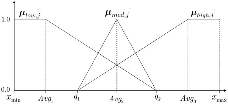
The 3 fuzzy membership functions μlow,j, μmed,j and μhigh,j, which were used to replace expression values of feature (gene) j during fuzzy classification.
| (2) |
| (3) |
| (4) |
The above computations result in 3 fuzzy sets (vectors) μlow,j, μmed,j and μhigh,j of length n which replace the original input feature. During classification with fuzzy features, the incorporation of new features was incremented in sets of size 3Ω (Ω − 1)/2. Figure 1 illustrates the values of the membership functions as a function of xij. When features are fuzzified using the methods described above the classifiation is called “fuzzy,” whereas without feature fuzzification, classification is called “crisp.”
1.4 Classification Analysis
Fourteen classifiers were employed: k nearest neighbor (kNN), näive Bayes classifier (NBC), linear discriminant analysis (LDA), quadratic discriminant analysis (QDA), learning vector quantization (LVQ1), logistic regression (LOG), polytomous logistic regression (PLOG), artificial neural networks (ANN), particle swarm optimization (PSO), constricted particle swarm optimization (CPSO), kernel regression (RBF), radial basis function networks (RBFN), gradient descent support vector machines (SVMGD), and least squares support vector machines (SVMLS).
1.4.1 k-Nearest Neigbor (kNN)
The k-nearest neighbor classifier (kNN) is based on the Euclidean distance between a test sample and the specified training samples[24]. A test sample x is assigned to the class ω of its nearest neighbor, where mi is a nearest neighbor to x if the distance
| (5) |
where D(mj, x) = ||mj − xi|| is the Euclidean distance. The k-nearest neighbors to x are identified and the decision rule D(x ⇝ω) is to assign sample x to the class ω which is the most popular among the k nearest training samples. In this study, we set k=4 for all runs, and thus the classifier is noted as 4NN.
1.4.2 Näive Bayes Classifier (NBC)
Näive Bayes classifiers (NBC) were developed from probability-based rules derived from Bayes Rule, and therefore are able to perform efficiently with minimum error rate[24]. Our application of NBC was based entirely on discretizing expression values across samples into categorical codes for quantiles. Training for NBC first requires calculation of the 3 cutpoints of quartiles of each training feature over the training samples independent of class, which characterizes the distribution of each training feature considered. We used an array of size # training features × 3 to store the 3 quartile cutpoints for each feature. Using the cutpoints for quantiles of each feature, we transformed continuous feature values into categorical quantile codes and tabulated cell counts n(j, qj, ω), which is the number of samples having a quantile value of qj (qj = 1, 2, 3, 4) for the j th feature in class ω. At program start, each cell count is set to n(j, qj, ω) = 1 in order to prevent multiplication by zero when probabilities are determined during testing. This was performed for all training samples. During testing, we used the array of quantile cutpoints to transform each test sample’s continuous feature values into categorical quantile values of qj =1,2,3 or 4. The assignment of a test sample x to a specific class was based on the posterior probability of class ω, given as
| (6) |
where P(ω) is the class prior and P(x|ω) is the conditional probability density. Note that P(ω) is constant and therefore only P(x|ω) requires maximization. Thus we compute
| (7) |
where n(ω) is the number of samples in class ω used for training and p is the number of training features. It is clear that we are using the categorical quantile values of qj for each feature of the test sample to obtain the probability n(j, qj, ω)/n(ω), which is multiplied together for all features. The decision rule for the test sample x is
| (8) |
1.4.3 Linear Discriminant Analysis (LDA)
Linear discriminate analysis (LDA) first requires calculation of the p × p class-specific variance-covariance matrices Sω[25]. For a given set of p features, calculation of Sω is based on samples having class label ω. The diagonal elements of the matrix Sω are written in the form
| (9) |
and off-diagonal elements as
| (10) |
where is the variance for feature j among samples in class ω, sjk is the co-variance between features j and k among samples in class ω, and ȳj is the mean of feature j for samples in class ω. The major assumption for LDA is that the variance-covariance matrices are all equal, that is, S1 = S2 = … = SΩ. Using the class-specific variance-covariance matrices, we calculate the pooled covariance matrix as
| (11) |
For a given sample y represented by a p × 1 vector of feature values, the distance from the sample to the centroid of class ω is defined as
| (12) |
where ȳω is a p × 1 vector of mean feature values for samples in class ω, for which the individual elements are
| (13) |
The decision rule D(y ⇝ω) is to assign sample y to the class for which Dω(y) is the smallest.
1.4.4 Quadratic Discriminant Analysis (QDA)
When the covariance matrices are not equal, the distance from each sample to class centroids is biased by large variance values on the matrix diagonals[25]. To minimize this bias among unequal covariance matrices, we replace the pooled covariance matrix Spl in (12) with the class specific covariance matrices in the form
| (14) |
The same decision rule is used as before, in which sample y is assigned to the class for which Dω(y) is the smallest.
1.4.5 Learning Vector Quantization (LVQ1)
Supervised classification under learning vector quantization 1 (LVQ1) involves a punishment-reward method for moving prototypes toward samples with the same class and away from samples with different class labels [26]. We first specified the number of prototypes per class. This can be done arbitrarily or through a grid search over the specified number of prototypes. Some authors recommend setting the number of prototypes the same in each class, however, this may be uncecessary since there may be more(fewer) prototypes than are needed for class separability. Nevertheless, we used a fixed value of k = 2 prototypes per class derived from k-means cluster analysis.
Let xi be the i th sample (i = 1, 2, …, n) and mj (j = 1, 2, …, P) be a prototype. During the initial iteration LVQ1 selects the first sample xi and derives the distance to each prototype mj among all P prototypes in the form
| (15) |
The closest prototype is then updated according to the rule
| (16) |
where mj is the prototype closest to sample xi and α(t) is the learning rate at the tth iteration (t = 1, 2, …, Tmax). Under the above updating rule the closest prototype is rewarded if its class label is the same as the class label of the sample and punished if different. A suitable choice for the learning rate α(t) is
| (17) |
Reliable results for LVQ were obtained using a value of α0=0.1 and Tmax = 50 iterations. The above calculations at iteration t were repeated for the remaining samples, each time looping over all P prototypes to find the closest prototype. This was then carried out over Tmax total iterations. During testing, the decision rule is to assign sample x to the class of which the closest prototype belongs shown as
| (18) |
1.4.6 Logistic Regression (LOG)
Logistic regression (LOG) employs a maximum likelihood optimization approach to model all classification problems in the form of multiple 2-class problems[27]. For example, a 4-class problem equates to 6 = [4(4 − 1)/2] 2-class problems. Assume a training scenario comparing training samples from class j and class k(k ≠ j, k = 1, 2, …, Ω ). Set yi = 0 if the i th sample is from class j and yi = 1 if the ith sample is from class k. Logistic regression first requires computation of the logit g1(xi) = β0 + β1xi1 + β2xi2 +···+ βpxip, which is hinged to regression coefficients modeled during the fitting procedure. Maximum likelihood modeling is performed and after convergence the probability that a test sample x is in class j is P(j |x) = P(y = 0|x) = 1/[1 + eg1(x)] and the probability of class k membership is 1 − P(j |x). Hence, the two decision rules for test sample x are Djk = P(j |x) and Dkj = 1 − Djk. The intermediate decision rule for class j is
| (19) |
and the final decision rule for test sample x is
| (20) |
1.4.7 Polytomous Logistic Regression (PLOG)
The 2-class and multiclass data sets used were handled straightforwardly with polytomous logistic regression, where multiclass problems were not reduced to multiple 2-class problems. Instead, polytomous logistic regression (PLOG) handles all of the classes considered in a single run. In polytomous logistic regression, only Ω −1 logits are needed, where the general equation for the logit is gj (xi) = βj0+ βj1xi1+ βj2xi2+···+ βjpxip = log[P(yij = j |xi )/P(yij = 0|xi ). Because yi0 drops out of the likelihood equation, only classes ω = 2, 3, …, Ω are needed for setting yij for each sample. For example, during a 4-class problem analysis, a training sample from class 2 would require the coding yi1 = 1, yi2 = 0, and yi3 = 0 in order to represent classes 2–4. After the model is fit, the committee vote (y = 0, 1, …, Ω − 1) for class 1 is , and for all other classes. The final decision rule for class j is
| (21) |
1.4.8 Artificial Neural Networks (ANNs)
Artificial neural networks (ANNs), otherwise known as multilayer perceptrons (MLPs), are machine-based learning models which simulate information processing performed by the brain. ANNs consist of neurons, or cells, interconnected by synaptic weights that filter and transmit information in a supervised fashion into order to acquire knowledge that can be stored in memory. After adapting to an environment in which an ANN is embedded, the stored knowledge can be generalized to future experiences to predict outcome based on input stimuli.
During the feed-forward training input vectors for each sample x were clamped to the input nodes. Features were standardized over the training samples considered in each run to ensure the same scale. The initial random connection weights were in the range [−0.5, 0.5]. Node outputs at the hidden layer were based on a logistic activation function in the form
| (22) |
where uj is the input to hidden node j and vj is the output. Using the output of neuron j in the hidden layer, the total input to the kth neuron in the output layer is
| (23) |
where is the connection weight between neuron j in the hidden layer and neuron k in the output layer. The output of neuron k (k = 1, 2, …, Ω) in the output layer was obtained using the softmax function
| (24) |
which normalizes all the zk so that they sum to unity. Finally, the error is determined as the total sum-of-squares based on the difference between the output vector and the “target” vector representing the true output, given as
| (25) |
where ck is the kth element in the binary vector c with known class for this training sample. For a 4-class example problem, examples of the four possible target vectors c for training samples known to be in classes 1, 2, 3, or 4 are c = (1, 0, 0, 0), c = (0, 1, 0, 0), c = (0, 0, 1, 0), and c = (0, 0, 0, 1).
1.4.8.1 Cycles and Epochs (Sweeps)
Node outputs described in (22) and (24) only apply to forward propagation of information for a single sample from the time the input vector is clamped to the input nodes up to the last output step. After the feed forward step for a sample, gradient descent back-propagation learning is performed using partial derivatives of the outputs at the hidden and output layers w.r.t. connection weights[28]. A cycle constitutes a sequence of forward and backward passes for one sample. A complete cycle of training using all of the samples is termed a sweep. After the initial assignment of random weights and several sweeps through the training samples, classification error will start to decrease. As this occurs, the ANN will be learning the relationship between the input and output vectors. For most data, a marked reduction in error usually occurs within 25 sweeps, so by default we used 100 sweeps. We have observed substantial monotonically decreasing reductions in error to near zero levels for 50 sweeps[28], so use of 100 should be less problematic. During testing, the feature values of each test sample x are clamped to the input nodes and propagated through the connections to derive the target vector z. The decision rule D(x ⇝ω) is to assign x into the class for which zk is the greatest. A grid search was employed for each ANN model in which the learning rate ε and momentum α ranged from 2−9, 2−8, …, 2−1. The grid search for ANNs also included an evaluation of error for a variable number of hidden nodes in the single hidden layer, which ranged from the number of training features (i.e., the length of input vector for each sample) down to the number of output nodes, incremented by −2. In cases when there were multiple values of grid search parameters for the same error rate, we used the median value.
1.4.9 Particle Swarm Optimization (PSO)
Particle swarm optimization (PSO) was introduced by Kennedy and Eberhart in 1995 [29] as a new optimization tool for stochastic searching in multimodal space. PSO is modeled after the behavior of migrating flocks of birds or feeding behaviors of schools of fish, in which “particles” fly through the multidimensional space exchanging information along the way in order to influence others movements to find a global maximum. Each particle has a cognitive memory about the position where the best fitness occurred, as well as a social memory on where the best fitness occurred among all members of the swarm. Particle travel is hinged to the velocity based on the last position, the cognitive and social memories, and randomness.
Let each particle form a 2 × Ω × p array, where Ω is the number of classes and p is the number of features. Let the position and velocity vectors for particle l be . The class-specific particle position is and the class-specific particle velocity is . At each iteration, the fitness [30] is based on
| (26) |
where n is the number of training samples and ω(xi) is the class of sample xi. The velocity update is
| (27) |
where w is the inertia factor, c1 is the cognitive parameter and c2 is the social parameter, bl(t) is the best historical fitness for particle l, and bg(t) is the global best particle. The inertia at iteration t is w(t) = wstart − (wstart − wend)t/Tmax. The particle position update is rl (t + 1) = rl (t) + vl (t + 1).
1.4.9.1 Constricted Particle Swarm Optimization (CPSO)
In constricted particle swarm optimization (CPSO), the inertia factor w in (27) was replaced with the constriction factor κ defined as
| (28) |
where ϕ, = c1 + c2, ϕ > 4. The velocity update then becomes
| (29) |
The decision rule for class j of a test sample x is
| (30) |
Parameter values for PSO were set to: #numparticles = 50, Tmax= 300, υmin = −0.05, υmax = 0.05, c1 = 2, c2 = 2, wmin = 0.4, and wmax = 0.9. Whereas for CPSO, the parameters were #numparticles = 30, Tmax = 150, υmin = −0.05, υmax = 0.05, c1 = 2.05, c2 = 2.05, wmin = 0.4, and wmax = 0.9.
1.4.10 Kernel Regression (RBF) and RBF Networks (RBFN)
Kernel regression (RBF) employs kernel tricks in a least squares fashion to determine coefficients that reliably predict class membership when multipled against kernels for test samples. Multiple class problems are solved using all possible 2-class problems. First, k-means cluster analysis is performed on all of the training samples to determine the centers. Let N be the number of training samples and M be the number of centers extracted from the training data. Coefficients for kernel regression are determined using the least squares model
| (31) |
where H is an N × M matrix with elements hij = K(xi, cj ), and y a N × 1 vector with yi set to 1 for training samples in the first class and yi set to −1 for samples in the second class being compared in the 2-class problem. Because HT is an M × N matrix, the inverse of the dispersion matrix (HTH)−1 is an M × M matrix. When cross multiplied with HT y, which is M × 1, the resulting vector α is an M × 1 vector. The predicted y for a test sample is based on the sum product of the kernel K(x, cj) for the test sample and each center by the respective αj for the j th center, shown as
| (32) |
A positive value of y denotes membership in the first class and a negative value of y reflects membership in the second class.
The radial basis function network (RBFN) employed the same matrix algebra as kernel regression, but was based on the kernel K(xi, cj) = ||xi − cj || and not K(xi, cj) = exp(−||xi − cj||), since the former commonly provided better results.
1.4.11 Support Vector Machines (SVM)
Support vector machines (SVMs) offer many advantages over other classifiers, for example, they maximize generalization ability, avoid local maxima, and are robust to outliers. However, their disadvantages are that they do not extend easily to multiclass problems, can require long training times when quadratic programming is used, and are sensitive to model parameters the same way ANNs are sensitive to the number of hidden layers and number of nodes at each hidden layer.
For multiple class problems, all possible 2-class comparisons were used. Training samples were coded as a y vector, where yi = 1 for the first class and yi = −1 for the second class. We used a gradient descent-based [31] and least squares[32] approach to SVM. The gradient descent L1 soft norm SVM (SVMGD) employed the recursive relationship for the ith training sample in the form
| (33) |
where α is a sample × 1 vector of Lagrange multipliers, and K(xi, xi) is the kernel.
The least squares SVM (SVMLS) was an L2 norm SVM, (i.e., ) based on the matrix operation
| (34) |
for which the intercept term is
| (35) |
where Ω ij = yiyj K(x, xT) + δij / C, C is the margin parameter, δij =1 if i = j or 0 if i ≠ j,δij/C is added to the diagonal of K(x, xT). The margin parameter C controls the trade-off between minimizing the norm of the slack vectors, e.g., ξi = αi/C, and maximizing the target margin. For SVMLS, all αi are support vectors. A weighted exponentiated RBF kernel was employed to map samples in the original space into the dot-product space, given as , where m=#features. Such kernels are likely to yield the greatest class prediction accuracy providing that a suitable choice of γ is used. To determine an optimum value of γ for use with RBF kernels, a grid search was done using incremental values of γ from 2−15, 2−13, …, 23 in order to evaluate accuracy for all training samples. We also used a grid search in the range of 10−2, 10−1, …, 104 for the margin parameter C. Median parameter values were used whenever there were multiple grid search values observed at the same error rate. The optimal choice of C is based on the grid search for which classification accuracy is the greatest, resulting in the optimal value for the separating hyperplane and minimum norm ||ξ|| of the slack variable vector. The decision function for class j is
| (36) |
where
| (37) |
and S is the set of bound support vectors for which αi = C, and b = 1/UΣj ∈U [yi− Σi∈S αi yiK(xi, xj)] Ω where U are the unbounded support vectors (0 < αi < C). In least squares SVM, b is directly solved during matrix operations. The decision rule for test sample x is
| (38) |
1.5 Classification Runs
Using the 9 data sets, we performed 4 runs for each data set. These consisted of no feature standardization or fuzzification, only standardization, only fuzzification, or both. Because we varied sample size and feature set size, within each of these four runs there were 60 runs for AMLALL2, 60 for Brain, 60 for BreastA, 60 for BreastB, 60 for colon, 60 for lung, 60 for prostate, 36 for MLL Leukemia, and 18 for SRBCT, for a total of 474. Therefore, there were 474 × 4 = 1,896 runs per classifier. Multiplying 1,896 by the 14 classifiers used resulted in 26,544 total classification runs, each of which resulted in an AUC value. These 26,544 AUC values were used in regression analyses (see below). Taking a deeper look behind the scenes, we further ran each classifier 40 times for each set of randomly selected samples drawn, and another 40 times when the class labels were permuted (see below). Overall, we performed a total of 80 × 26, 544 = 2, 123, 530 classification runs.
1.6 Receiver Operator Characteristic (ROC) Curves
For each classifier, ROC curves were generated using randomly selected proportions of 10%, 20%, 30%, 40%, 50%, or 60% of the total number of input samples. During each iteration, classifier training was performed with the randomly selected samples and testing was performed on the remaining samples left out of training. Random selection of samples was also stratified to ensure uniform class representation to the extent possible. For a given sample size, we also varied the number of features used based on the best ranked N features chosen. The number of steps used for varying the feature count was set equal to 20=(Ω (Ω − 1)/2), so that no more than 20 features were used for any run.
For each fixed set of randomly selected training samples and features, the proportion of input samples was resampled B = 40 times in order generate 40 realizations (values) of observed and null accuracy. Mukherjee et al used B = 50 iterations during randomization tests to obtain SVM error rates for linear kernels based on 150 or all features for some of the same data sets [11]. Therefore, it is our belief that the cost-saving attempt to use 40 iterations for considerably more classification runs is appropriate. At each iteration, we first calculated accuracy based on the true class labels to obtain Accb (b = 1, 2, …, B), and then permuted class labels to obtain the null accuracy, . This provided B = 40 values of accuracy for the observed data and 40 values of accuracy for the null data. The mean μ and standard deviation σ of Accb and were then determined and used for generating 1000 quantiles of accuracy, based on the relationship μ+ N(0, 1)σ. Quantiles for the observed accuracy were termed xi and null accuracy termed . In order to calculate AUC, we needed to transform the lists of simulated accuracy quantiles into probability density functions. The pdf’s of xi and were each approximated by using kernel density estimation (KDE) with M = 1000 equally spaced bins over the range Δx = min{μ + 4σ, 1} − max{μ − 4σ, 0} based on the bin frequencies
| (39) |
where f(m) is the smoothed bin count for the mth bin, xi is the simulated accuracy quantile, xm is the lower wall of the mth bin, and h = 2 − 1.06σN−0.2 is the bandwidth[33]. K is the Gaussian kernel function defined as
| (40) |
where u = (xi − xm)/h. The smoothed histogram bin heights f (m) were normalized so that the approximate area under the curve was unity. KDE resulted in the pdf p(x) for the observed accuracy distribution and p(x*) for the null accuracy distribution. Construction of ROC curves assumed that p(x) was the “signal” while p(x*) was the “noise.” AUC was determined with the relationship . It is important to note that the minimum and maximum quantile values of accuracy for the null and alternative distributions were different. Thus, in the case of highly significant classification, the lowest quantile (accuracy) value of the alternative distribution will be greater than the greatest accuracy value in the null distribution. This is a common observation when using randomization tests for highly significant effect measures, where test statistics based on permuted labels are much lower than test statistics for the observed data.
1.7 Regression Modeling of Area Under the Curve (AUC)
A multiple linear regression model was used to regress AUC as the dependent variable on several parameters hypothesized to influence AUC for each classifier. That is, AUC was fitted separately for each classifier. The regression model used is given below:
| (41) |
where y is the AUC for the selected classifier, 1/#samplesis the inverse of the number of training samples used, 1/sum[−log(p)] is the inverse of the sum of the minus logarithm of p-values for features used based on the 2-class t-test, stdrepresents standardization of features values (0-no, 1-yes) using the mean and standard deviation over all input samples (not training samples), fuzzyrepresents fuzzification of the features used, and ε is the residual error. Fitted values of AUC for each classifier (regression model) were generated for a range of sample sizes (1–50), with and without feature standardization, with and without feature fuzzification, for low levels of feature statistical significance (1/sum[−log(p)]=1/50) and high levels (1/sum[−log(p)]=1/500) of feature statistical significance.
2 Results
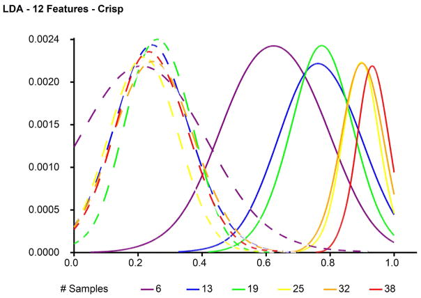
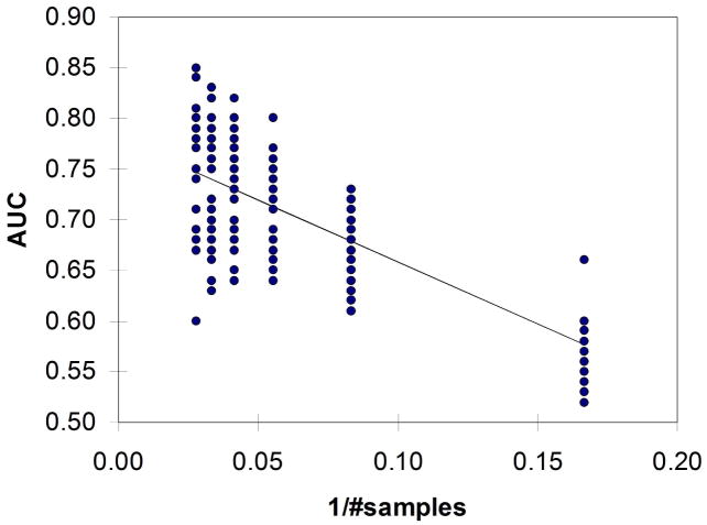
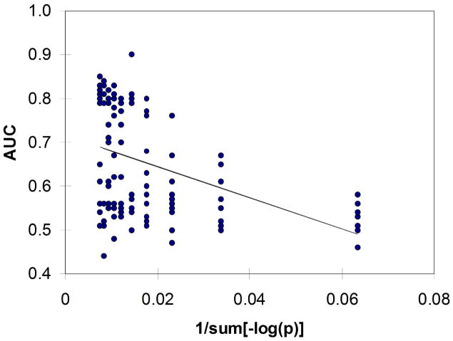
Figure 2 illustrates example results for the observed (signal) and null (noise) distributions of accuracy derived from classification with LDA using the top 12 features selected from the 4-class SRBCT data set. Figure 3 shows an example ROC curve generated from the signal and noise distributions shown in Figure 2. Figure 4 provides insight into an example linear fit of AUCon 1/#samplesfor the 4NN classifier and Figure 5 gives insight into the fit of AUC on 1/sum[−log(p)]. The clear decreasing trends shown in Figures 4 and 5 support the assumption for using the 1/x transform for the sample size and sum[−log(p)] parameters in multiple linear regression.
Fig. 2.
Example observed and null accuracy distributions derived from classification with LDA using the top 12 features selected from the 4-class SRBCT data set. Dotted lines -- - represent null accuracy distributions and solid lines —– represent observed accuracy distributions.
Fig. 3.
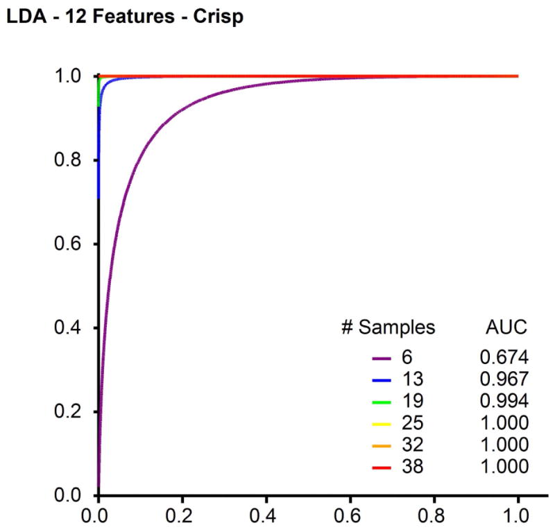
Example receiver operating characteristic (ROC) curve generated from pdf’s shown in Figure 2 for classification of 4-class SRBCT data using the top 12 features selected.
Fig. 4.
Example linear fit of AUC on 1/#samples for the 4NN classifier.
Fig. 5.
Example linear fit of AUC on 1/sum[−log(p)] for the ANN classifier.
Table 2 lists the regression coefficients and their standard errors for the multiple regression model. Use of the number of features used for AUC determination rather than sum[−log(p)] for the multiple features did not result in coefficients that were more explanatory and more significant. This was expected because the total statistical significance (i.e., sum[−log(p)]) among a set of best ranked N features can vary greatly with the number of features. The constant terms β0 listed in Table 2 suggest that at the greatest level of sample size, ANN resulted in the greatest fitted levels of AUC (90%), while PSO resulted in the lowest fitted AUC (72.1%). In addition, AUC values derived from 4NN were the most dependent on sample size, while PSO was the least. ANN depended on the total statistical significance of features used based on sum[−log(p)], whereas PSO was the least dependent. Standardization of features increased AUC by 8.1% for PSO and -0.2% for QDA, while fuzzification increased AUC by 9.4% for PSO and reduced AUC by 3.8% for QDA.
Table 2.
Regression coefficients (s.e.) for classifier-specific linear fits of AUC on 1/#samples, 1/sum[−log(p)], standardization of features (0-no,1-yes), and fuzzification of features (0-no,1yes). Coefficients in bold typeface represent strongest effect observed.
| Classifiera | β0(s.e.) | β1/samples(s.e.) | β1/sum[−log(p)] (s.e.) | βstd (s.e.) | βfuzzy (s.e.) |
|---|---|---|---|---|---|
| 4NN | 0.886(0.006)* | −1.207(0.037)* | −3.252(0.192)* | 0.008(0.005) | 0.032(0.005)* |
| NBC | 0.877(0.006)* | −0.892(0.036)* | −2.612(0.188)* | 1E-05(0.005) | −0.007(0.005) |
| LDA | 0.823(0.006)* | −0.273(0.041)* | −3.144(0.210)* | 0.002(0.005) | 0.019(0.005)* |
| QDA | 0.795(0.006)* | −0.783(0.036)* | −1.666(0.184)* | −0.002(0.005) | −0.038(0.005)* |
| LVQ1 | 0.850(0.006)* | −0.021(0.038) | −4.345(0.195)* | 0.009(0.005)* | 0.043(0.005)* |
| LOG | 0.756(0.007)* | −0.159(0.043)* | −3.709(0.223)* | 0.050(0.006)* | 0.081(0.006)* |
| PLOG | 0.789(0.006)* | −0.109(0.04)* | −3.606(0.205)* | 0.026(0.005)* | 0.054(0.005)* |
| ANN | 0.900(0.008)* | −0.698(0.049)* | −6.297(0.254)* | 1E-05(0.007) | −0.025(0.007)* |
| PSO | 0.721(0.005)* | b | −2.530(0.203)* | 0.081(0.006)* | 0.094(0.006)* |
| CPSO | 0.859(0.005)* | −0.104(0.033)* | −2.760(0.169)* | 0.017(0.004)* | 0.016(0.004)* |
| RBF | 0.796(0.006)* | −0.386(0.039)* | −3.380(0.203)* | 0.049(0.005)* | 0.056(0.005)* |
| RBFN | 0.858(0.006)* | −0.344(0.036)* | −3.402(0.184)* | 0.009(0.005)* | 0.010(0.005)* |
| SVMGD | 0.837(0.007)* | −0.126(0.043)* | −4.480(0.225)* | 0.012(0.006)* | 0.039(0.006)* |
| SVMLS | 0.845(0.007)* | −0.005(0.044) | −4.729(0.226)* | 0.004(0.006) | 0.035(0.006)* |
p < 0.05
A total of 1,896 values of AUC (records) were used for each classifier-specific linear fit.
For PSO, #samplesrather than 1/#sampleswas used and resulted in β#samples = −0.001 and s.e.(β#samples) = 0.0002 suggesting a decrease in AUC with increasing sample size, and was therefore not used for determination of fitted AUC.
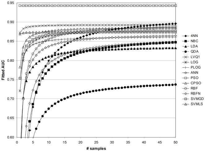
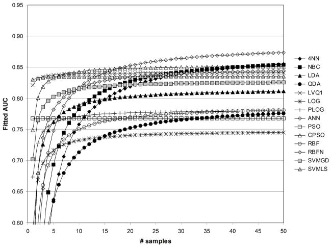
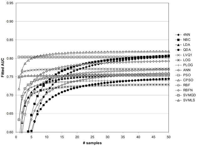
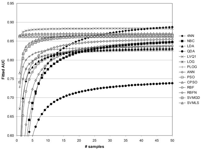
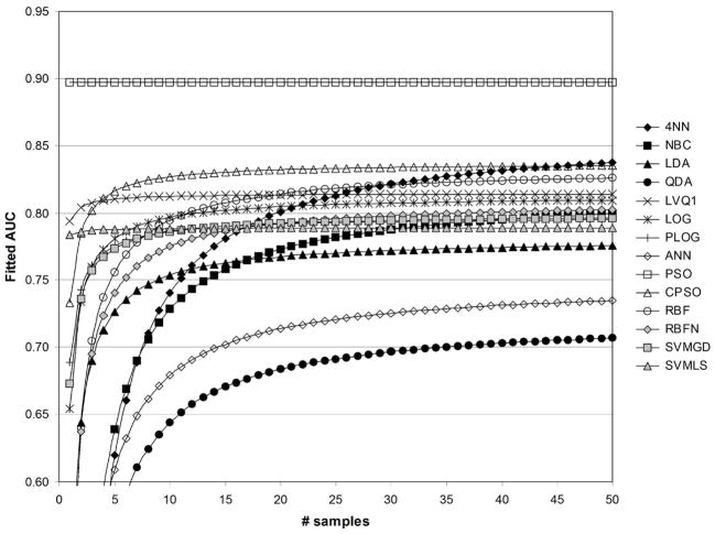
In Figures 6–13, the fitted values of AUC as a function of samples size with and without feature standardization and feature fuzzification are shown for values of 1/sum[−log(p)]=1/50 and 1/sum[−log(p)]=1/500. Fitted AUC values are based on ((41)) and regression coefficient values in Table 2. Figures 6 and 7 show fitted AUC when no feature standardization or fuzzification is performed. In both these figures, one can note the strong dependence of 4NN on sample size, since sample size had the strongest effect on AUC obtained with 4NN (see Table 2). In addition, the switch from Figure 6 to 7 involves using a greater significance level for the features selected, and here fitted AUC based on ANN is observed to change the greatest as 1/sum[−log(p)]changes from 1/50 to 1/500. This agrees with the results in Table 2, which show that the strongest effect of feature statistical significance was observed for ANN. Figure 6 shows that the greatest fitted values of AUC were obtained using the CPSO, followed by the LVQ1 classifier. The lowest values of fitted AUC were obtained using LOG and PLOG. Figure 7 shows that the greatest fitted values of AUC were obtained using ANN followed by CPSO. LVQ1 resulted in the third greatest level of fitted AUC. The lowest values of fitted AUC in Figure 7 were obtained using PSO followed by LOG.
Fig. 6.
Fitted values of AUC as a function of sample size, for 1/sum[−log(p)]=1/50, without standardization ( std=0), and without fuzzification ( fuzzy=0).
Fig. 13.
Fitted values of AUC as a function of sample size, for 1/sum[−log(p)]=1/500, with standardization ( std=1), and with fuzzification ( fuzzy=1).
Fig. 7.
Fitted values of AUC as a function of sample size, for 1/sum[−log(p)]=1/500, without standardization ( std=0), and without fuzzification ( fuzzy=0).
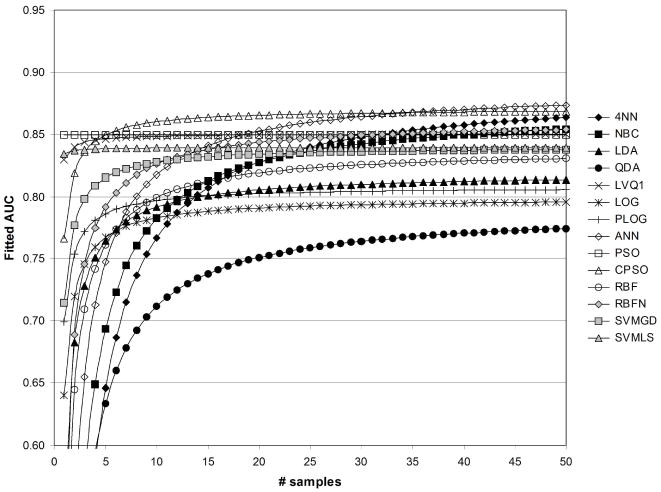
Figures 8 and 9 show fitted AUC when only feature standardization is performed. Because the strongest effect of feature standardization was observed for PSO (Table 2), the large increase observed for fitted AUC for PSO in Figures 8 and 9 was expected. Figure 8 illustrates that the greatest fitted values of AUC were obtained using the CPSO followed by PSO. The lowest values of fitted AUC were obtained using LOG and QDA. Figure 9 shows that fitted AUC was the greatest for ANN followed by CPSO. LVQ1 resulted in in the third greatest level of fitted AUC. The lowest values of fitted AUC in Figure 9 were obtained using QDA followed by LOG.
Fig. 8.
Fitted values of AUC as a function of sample size, for 1/sum[−log(p)]=1/50, with standardization ( std=1), and without fuzzification ( fuzzy=0).
Fig. 9.
Fitted values of AUC as a function of sample size, for 1/sum[−log(p)]=1/500, without standardization ( std=1), and without fuzzification ( fuzzy=0).
Figures 10 and 11 shows fitted AUC when only feature fuzzification is performed. Note that, in Table 2, the strongest effect of feature fuzzification was observed for PSO, and accordingly the large increase observed for fitted AUC for PSO in Figures 10 and 11 was expected. Figure 10 indicates the greatest fitted values of AUC were obtained using the CPSO followed by PSO. The lowest fitted values of AUC were obtained using the QDA and ANN. Figure 11 shows that the greatest fitted values of AUC were obtained using LVQ1 followed by CPSO. The lowest values of fitted AUC in Figure 11 were obtained using QDA followed by PSO.
Fig. 10.
Fitted values of AUC as a function of sample size, for 1/sum[−log(p)]=1/50, without standardization ( std=0), and with fuzzification ( fuzzy=1).
Fig. 11.
Fitted values of AUC as a function of sample size, for 1/sum[−log(p)]=1/500, without standardization ( std=0), and with fuzzification ( fuzzy=1).
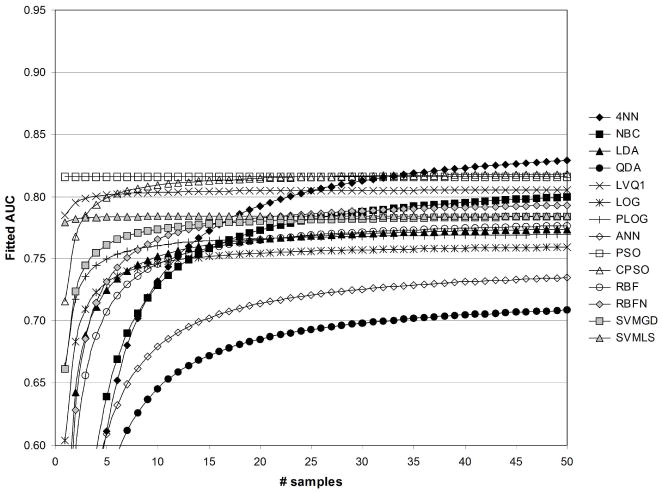
Figures 12 and 13 illustrate fitted AUC when both feature standardization and feature fuzzification is performed. Not surprisingly, PSO was expected to result in the greatest levels of fitted AUC following feature standardization and fuzzification because of the strong effects for these parameters listed in Table 2. Figure 12 reflects that the greatest fitted values of AUC were obtained using the PSO followed by CPSO. The lowest values of fitted AUC were obtained using QDA and ANN. Figure 13 shows that the greatest fitted values of AUC were obtained using PSO then LVQ1. The lowest values of fitted AUC in Figure 13 were obtained using QDA followed by LDA.
Fig. 12.
Fitted values of AUC as a function of sample size, for 1/sum[−log(p)]=1/50, with standardization ( std=1), and with fuzzification ( fuzzy=1).
3 Discussion and Conclusions
The effects of sample size, feature significance, feature standardization, and feature fuzzification varied over the classifiers used. Particle swarm optimization (PSO) and constricted particle swarm optimization (CPSO) were the best performing classifiers resulting in the greatest levels of fitted AUC. LVQ1 typically resulted in the second greatest levels of fitted AUC. Quadratic discriminant analysis (QDA) and logistic regression (LOG) commonly resulted in the least levels of fitted AUC. Artificial neural networks (ANN) was on occasion the best and worst classifier. Table 3 lists the two best and two worst classifiers for fitted AUC values shown in Figures 6–13.
Table 3.
List of classifiers which resulted in the least and greatest levels of fitted AUC.
| Feature standardization | Feature fuzzification | Feature 1/sum[−log(p)] | Fitted AUC | |
|---|---|---|---|---|
| Least | Greatest | |||
| No | No | 1/50 | LOG, PLOG | CPSO, LVQ1 |
| 1/500 | QDA, LVQ1 | ANN, CPSO | ||
| Yes | No | 1/50 | QDA, LVQ1 | PSO, CPSO |
| 1/500 | QDA, LVQ1 | PSO, CPSO | ||
| No | Yes | 1/50 | QDA, ANN | PSO, LVQ1 |
| 1/500 | QDA, LOG | LVQ1, SVMLS | ||
| Yes | Yes | 1/50 | QDA, ANN | PSO, CPSO |
| 1/500 | QDA, LDA | PSO, LVQ1 | ||
In Table 3, the PSO and CPSO classifiers were listed 5 out of 8 times with the greatest fitted AUC levels among the 8 combinations of analyses. Without standardization or fuzzification of features, CPSO outperformed PSO, which is in agreement with previous findings[34]. Use of the constriction factor in CPSO prevents particles from overshooting the search space (going outside of the galaxy being searched) and shortens the steps taken. When ϕ < 4, particles tend to orbit rather than converge, but when ϕ < 4, particles oscillate with quickly decaying amplitude[35]. LVQ1 was listed 4 times among the 8 types of runs enumerated in Table 3. ANN and SVMLS were each listed once among the 8 combinations of runs. For the lowest fitted values of AUC observed, QDA was listed 7 times among the 8 combinations of runs. LVQ1 was listed 3 times among the 8 combinations of runs, and LOG and ANN were each listed twice. PLOG and LDA were listed once among the 8 types of runs for yielding the lowest levels of AUC.
Other general observations regarding the classifiers were the that fitted AUC values for LDA were greater than those for QDA, and QDA was one of the worst performing classifiers. The performance of LDA and QDA will suffer whenever features are highly correlated, causing the variance-covariance matrix to be singular. Singular variance-covariance matrices have at best one eigenvalue which is equal to the first principal component, resulting in a degeneration of the Mahalanobis distance. In addition, QDA assumes unequal class-specific variance-covariance matrices, whereas LDA uses the pooled variance-covariance matrix which may be less degenerate. PLOG also resulted in fitted AUC values that were greater than those produced by use of LOG when both standardization and fuzzification of features was not performed. This indicates that all-at-once classification with PLOG using a likelihood function tailored to multiple outcomes was better than using pairwise classification based on binary outcomes required with LOG. ANN performed quite well and was influenced the most by statistical significance of the features used. Standardization did not effect ANN because we always standardized features with ANN. Fuzzification degraded performance of ANN as well as NBC and QDA. RBFN, which employs a distance kernel, resulted in fitted AUC values exceeding those for RBF, which used a linear kernel. The linear kernel of RBF did, however, perform better when both feature standardization and fuzzification were used. The SVMLS consistently outperformed the SVMGD, especially at lower sample sizes. When compared with gradient descent SVMs, which are of the L1 soft norm type and convex, least squares SVMs are L2 soft norm and are strictly convex, providing a unique solution that is typically the same or better. However, because least squares SVMs employ equality constraints rather than inequality contraints, they are more dependent on the data and tend to be more sensitive to outliers[32]. Our plots of fitted AUC values for SVMGD are very similar to error plots for SVMs for the same data sets reported by Mukherjee et al[11].
The major conclusions of this study are as follows. When generating AUC values, the 4NN classifier depended the most on sample size, while ANN depended the most on statistical significance of features used. AUC based on PSO is increased by 8.1% and 9.4% from the use of feature standardization and feature fuzzification, respectively. AUC based on CPSO was not as sensitive to standardization and fuzzification as PSO was. Lastly, LVQ1 performed surprisingly well, and essentially produced fitted AUC levels that tied AUC based on PSO when either feature standardization or fuzzification were performed, but not both. However, PSO substantially outperformed all other classifiers when both feature standardization and fuzzification were performed. In consideration of the data sets used and factors influencing AUC which were investigated, if low-expense computation is desired then LVQ1 is recommended. However, if computational expense is of less concern, then PSO or CPSO is recommended.
Table 1.
Data sets used for classification analysis.
| Cancer site | Classes | Samples | Features | Reference |
|---|---|---|---|---|
| Brain | 2 | 60 (21 censored, 39 failures) | 7,129 | Pomeroy et al[12] |
| Prostate | 2 | 102 (52 tumor, 50 normal) | 12,600 | Singh et al[13] |
| Breast | 2 | 15 (8 BRCA1, 7 BRCA2) | 3,170 | Hedenfalk et al. [14] |
| Breast | 2 | 78 (34 relapse, 44 non-relapse) | 24,481 | van ’t Veer et al[15] |
| Colon | 2 | 62 (40 negative, 22 positive) | 2,000 | Alon et al[16] |
| Lung | 2 | 32 (16 MPM, 16 ADCA) | 12,533 | Gordon et al[20] |
| Leukemia | 2 | 38 (27 ALL, 11 AML) | 7,129 | Golub et al [21] |
| Leukemia | 3 | 57 (20 ALL, 17 MLL, 20 AML) | 12,582 | Armstrong et al[22] |
| SRBCT | 4 | 63 (23 EWS, 8 BL, 12 NB, 20 RMS) | 2,308 | Khan et al[23] |
Acknowledgments
L.E.P was supported by US National Cancer Insititute (NIH) grant K22-CA100289-03.
References
- 1.Tibshirani RJ. A simple method for assessing sample sizes in microarray experiments. BMC Bioinformatics. 2006;7(1):106. doi: 10.1186/1471-2105-7-106. [DOI] [PMC free article] [PubMed] [Google Scholar]
- 2.Page GP, Edwards JW, Gadbury GL, Yelisetti P, Wang J, Trivedi P, Allison DB. The PowerAtlas: a power and sample size atlas for microarray experimental design and research. BMC Bioinformatics. 2006;7:84. doi: 10.1186/1471-2105-7-84. [DOI] [PMC free article] [PubMed] [Google Scholar]
- 3.Seo J, Gordish-Dressman H, Hoffman EP. An interactive power analysis tool for microarray hypothesis testing and generation. Bioinformatics. 2006;22(7):808–814. doi: 10.1093/bioinformatics/btk052. [DOI] [PubMed] [Google Scholar]
- 4.Tsai PW, Lee ML. Split-plot microarray experiments: issues of design, power and sample size. Appl Bioinformatics. 2005;4(3):187–194. doi: 10.2165/00822942-200504030-00003. [DOI] [PubMed] [Google Scholar]
- 5.Li SS, Bigler J, Lampe JW, Potter JD, Feng Z. FDR-controlling testing procedures and sample size determination for microarrays. Stat Med. 2005;24(15):2267–2280. doi: 10.1002/sim.2119. [DOI] [PubMed] [Google Scholar]
- 6.Jung SH, Bang H, Young S. Sample size calculation for multiple testing in microarray data analysis. Biostatistics. 2005;6(1):157–169. doi: 10.1093/biostatistics/kxh026. [DOI] [PubMed] [Google Scholar]
- 7.Wang SJ, Chen JJ. Sample size for identifying differentially expressed genes in microarray experiments. J Comput Biol. 2004;11(4):714–726. doi: 10.1089/cmb.2004.11.714. [DOI] [PubMed] [Google Scholar]
- 8.Tsai CA, Wang SJ, Chen DT, Chen JJ. Sample size for gene expression microarray experiments. Bioinformatics. 2005;21(8):1502–1508. doi: 10.1093/bioinformatics/bti162. [DOI] [PubMed] [Google Scholar]
- 9.Wei C, Li J, Bumgarner RE. Sample size for detecting differentially expressed genes in microarray experiments. BMC Genomics. 2004;5(1):87. doi: 10.1186/1471-2164-5-87. [DOI] [PMC free article] [PubMed] [Google Scholar]
- 10.Hwang D, Schmitt WA, Stephanopoulos G, Stephanopoulos G. Determination of minimum sample size and discriminatory expression patterns in microarray data. Bioinformatics. 2002;18(9):1184–1193. doi: 10.1093/bioinformatics/18.9.1184. [DOI] [PubMed] [Google Scholar]
- 11.Mukherjee S, Tamayo P, Rogers S, Rifkin R, Engle A, Campbell C, Golub TR, Mesirov JP. Estimating dataset size requirements for classifying DNA microarray data. J Comput Biol. 2003;10(2):119–142. doi: 10.1089/106652703321825928. [DOI] [PubMed] [Google Scholar]
- 12.Pomeroy SL, Tamayo P, Gaasenbeek M, Sturla LM, Angelo M, McLaughlin ME, Kim J-YH, Goumnerovak LC, Blackk PM, Lau C, Allen JC, ZagzagI D, Olson JM, Curran T, Wetmore C, Biegel JA, Poggio T, Mukherjee S, Rifkin R, Califanokk A, Stolovitzkykk G, Louis DN, Mesirov JP, Lander ES, Golub TR. Prediction of central nervous system embryonal tumour outcome based on gene expression. Nature. 2002;415(6870):436–442. doi: 10.1038/415436a. [DOI] [PubMed] [Google Scholar]
- 13.Singh D, Febbo PG, Ross K, Jackson DG, Manola J, Ladd C, Tamayo P, Renshaw AA, D’Amico AV, Richie JP, Lander ES, Loda M, Kantoff PW, Golub TR, Sellers WR¿. Gene expression correlates of clinical prostate cancer behavior. Cancer Cell. 2002;1(2):203–209. doi: 10.1016/s1535-6108(02)00030-2. [DOI] [PubMed] [Google Scholar]
- 14.Hedenfalk I, Duggan D, Chen Y, et al. Gene-expression profiles in hereditary breast cancer. N Engl J Med. 2001;344:539–548. doi: 10.1056/NEJM200102223440801. [DOI] [PubMed] [Google Scholar]
- 15.van ’t Veer LJ, Dai H, van de Vijver MJ, He YD, Hart AA, Mao M, Peterse HL, van der Kooy K, Marton MJ, Witteveen AT, Schreiber GJ, Kerkhoven RM, Roberts C, Linsley PS, Bernards R, Friend SH. Gene expression profiling predicts clinical outcome of breast cancer. Nature. 2002;415:530–536. doi: 10.1038/415530a. [DOI] [PubMed] [Google Scholar]
- 16.Alon U, Barkai N, Notterman DA, Gish K, Ybarra S, Mack D, Levine AJ. Broad patterns of gene expression revealed by clustering of tumor and normal colon tissues probed by oligonucleotide arrays. Proc Natl Acad Sci USA. 1999;96(12):6745–6750. doi: 10.1073/pnas.96.12.6745. [DOI] [PMC free article] [PubMed] [Google Scholar]
- 17.Klir GJ, Yuan B. Fuzzy Sets and Fuzzy Logic. Upper Saddle River(NJ): Prentice-Hall; 1995. [Google Scholar]
- 18.Dubois D, Prade H. Fundamentals of Fuzzy Sets. Boston(MA): Kluwer; 2000. [Google Scholar]
- 19.Pal SK, Mitra P. Pattern Recognition Algorithms for Data Mining: Scalability, Knowledge Discovery and Soft Granular Computing. Boca Raton(FL): Chapman & Hall; 2004. [Google Scholar]
- 20.Gordon GJ, Jensen RV, Hsiao LL, Gullans SR, Blumenstock JE, Ramaswamy S, Richards WG, Sugarbaker DJ, Bueno R. Translation of microarray data into clinically relevant cancer diagnostic tests using gene expression ratios in lung cancer and mesothelioma. Cancer Res. 2002;62(17):4963–5967. [PubMed] [Google Scholar]
- 21.Golub TR, Slonim DK, Tamayo P, Huard C, Gaasenbeek M, Mesirov JP, Coller H, Loh M, Downing JR, Caligiuri MA, Bloomfield CD, Lander ES. Molecular Classification of Cancer: Class Discovery and Class Prediction by Gene Expression. Science. 1999;286:531–537. doi: 10.1126/science.286.5439.531. [DOI] [PubMed] [Google Scholar]
- 22.Armstrong SA, Staunton JE, Silverman LB, Pieters R, den Boer ML, Minden MD, Sallan SE, Lander ES, Golub TR, Korsmeyer SJ. MLL translocations specify a distinct gene expression profile that distinguishes a unique leukemia. Nature Genetics. 2001;30(1):41–47. doi: 10.1038/ng765. [DOI] [PubMed] [Google Scholar]
- 23.Khan J, Wei JS, Ringner M, Saal LH, Ladanyi M, Westermann F, Berthold F, Schwab M, Antonescu CR, Peterson C, Meltzer RS. Classification and diagnostic prediction of cancers using gene expression profiling and artificial neural networks. Nature Med. 2001;7:673–679. doi: 10.1038/89044. [DOI] [PMC free article] [PubMed] [Google Scholar]
- 24.Mitra S, Acharya T. Data Mining, Multimedia, Soft Computing, and Bioinformatics. John Wiley; New York: 2003. [Google Scholar]
- 25.Rencher AC. Methods of Multivariate Analysis. Wiley; New York(NY): 2002. [Google Scholar]
- 26.Kohonen T. Self-Organizing Maps. Berlin: Springer; 2001. [Google Scholar]
- 27.Hosmer DW, Lemeshow S. Applied Logistic Regression. New York: John Wiley; 1989. [Google Scholar]
- 28.Peterson LE, Ozen M, Erdem H, Amini A, Gomez L, Nelson CC, Ittmann M. Proceedings of the 2005 IEEE Symposium on Computational Intelligence in Bioinformatics and Computational Biology. CIBCB 2005; San Diego, CA: Piscatawy(NJ): IEEE Computational Intelligence Society; 2005. Artificial neural network analysis of DNA microarray-based prostate cancer recurrence. [Google Scholar]
- 29.Kennedy J, Eberhart RC. Proceedings of IEEE International Conference on Neural Networks. Piscataway(NJ): 1995. Particle swarm optimization; pp. 1942–1948. [Google Scholar]
- 30.De Falco I, Della Cioppa A, Tarantino E. Evaluation of particle swarm optimization effectiveness in classification. Lecture Notes in Computer Science. 2006;3849:164–171. [Google Scholar]
- 31.Cristianini N, Shawe-Taylor J. Introduction to Support Vector Machines and Other Kernel-based Learning Methods. Cambridge: Cambridge Univ. Press; 2000. [Google Scholar]
- 32.Abe S. Advances in Pattern Recognition Series. Berlin: Springer; 2005. Support Vector Machines for Pattern Classification. [Google Scholar]
- 33.Fadda D, Slezak E, Bijaoui A. Density estimation with non-parametric methods. Astron Astrophys Suppl Ser. 1998;127:335. [Google Scholar]
- 34.Meissner M, Schmuker M, Schneider G. Optimized particle swarm optimization and its application to artificial neural network training. BMC Bioinformatics. 2006;7:125–136. doi: 10.1186/1471-2105-7-125. [DOI] [PMC free article] [PubMed] [Google Scholar]
- 35.Clerc M, Kennedy J. The particle swarm - Explosion, stability, and convergence in a multidimensional complex space. IEEE Transactions on Evolutionary Computation. 2002;6:58–73. [Google Scholar]


