Global-scale predictions of community and ecosystem properties from simple ecological theory

Abstract

We show how theoretical developments in macroecology, life-history theory and food-web ecology can be combined to formulate a simple model for predicting the potential biomass, production, size and trophic structure of consumer communities. The strength of our approach is that it uses remote sensing data to predict properties of consumer communities in environments that are challenging and expensive to sample directly. An application of the model to the marine environment on a global scale, using primary production and temperature estimates from satellite remote sensing as inputs, suggests that the global biomass of marine animals more than 10⁻⁵ g wet weight is 2.62×10⁹ t (=8.16 g m⁻² ocean) and production is 1.00×10¹⁰ t yr⁻¹ (31.15 g m⁻² yr⁻¹). Based on the life-history theory, we propose and apply an approximation for distinguishing the relative contributions of different animal groups. Fish biomass and production, for example, are estimated as 8.99×10⁸ t (2.80 g m⁻²) and 7.91×10⁸ t yr⁻¹ (2.46 g m⁻² yr⁻¹), respectively, and 50% of fish biomass is shown to occur in 17% of the total ocean area (8.22 g m⁻²). The analyses show that emerging ecological theory can be synthesized to set baselines for assessing human and climate impacts on global scales.

1. Introduction

Globally, communities and ecosystems are highly diverse, varying in species composition, biomass and productivity and their resilience to human impacts, environmental variation and change. However, these communities and ecosystems are also characterized by remarkably consistent relationships among variables such as species richness, abundance, range size and body size (Brown 1995; Gaston & Blackburn 2000; Kerr & Dickie 2001). Knowledge of these relationships, the reasons they evolve and their links to patterns of energy acquisition, transfer and use, can help to isolate the factors that account for differences among communities and ecosystems.

Here, we show how recent developments in macroecology, life-history theory and food-web ecology can be combined to formulate a simple model for predicting the potential biomass, production, size structure and trophic structure of consumer communities. The strength of this approach is that it uses remote sensing temperature and primary production (PP) data, available on global scales, to predict properties of consumer communities in environments that are challenging and expensive to sample directly. This approach builds on the observation that size distributions of animals in food webs largely reflect the availability and transfer of energy (Dickie et al. 1987; Brown & Gillooly 2003). These size distributions are often described as relationships between the logarithm of total abundance by body mass class and the logarithm of body mass, with individuals binned to body mass classes irrespective of species identity, and are dubbed size spectra (Sheldon & Parsons 1967).

Our example focuses on the marine environment and we use size spectra to describe the main flux of energy from primary producers to higher trophic levels. The rate and magnitude of flux depends on temperature and PP, parameters that are measured by remote sensing. Consumer production and biomass are determined from relationships that link body mass, temperature and mass-specific rates of production (Ernest et al. 2003; Brown et al. 2004). Our results provide a baseline for assessing human impacts and predicting the contribution of marine animals to biogeochemical processes, and can be compared with results from more complex community and ecosystem models applied at regional scales. We necessarily make many broad assumptions in an analysis of this type, and recognize and report on the scope to extend and further validate our approaches.

2. Material and methods

Biomass and production of consumer communities were calculated from estimates of the PP available to support them, accounting for the factors that affect the rate and efficiency of energy processing. These factors are (i) temperature that affects rates of metabolism and hence growth and mortality, (ii) the ratio of predator to prey body mass, which determines the number of steps in a food chain, and (iii) trophic transfer efficiency that measures how much energy is lost at each step. Biomass and production were estimated for 36×36 km grid cells covering all areas of the global oceans for which PP and temperature data were available.

(a) Production and size distribution of primary producers

PP was computed from satellite remote sensing measurements of chlorophyll a pigment (McClain et al. 2004) based on the approach of Longhurst et al. (1995). The sizes of phytoplankton cells that contribute to PP depend on the productivity of the ocean, with smaller phytoplankton dominating when PP is low (Agawin et al. 2000). To account for this, PP was allocated to 61 consecutive log phytoplankton body mass classes in an overall body mass range of W_m=10^−14.25–10^−5.25 g, where W_m is class midpoint wet mass. Within the overall body mass range, the position of the median body mass class (class 31 out of 61) was varied from 10^−11.25 to 10^−8.25 g to describe changes in the size distribution of phytoplankton. The location of the median body mass class was determined by the predicted contribution of small phytoplankton (picophytoplankton; here defined as cells of W_m<10^−11.35, equivalent spherical diameter approx. 2 μm) production (P_s) to total PP (P_p), based on the analysis of Agawin et al. (2000), where

$$P_{\text{s}}(\%)=(12.19\text{log}{P}_{\text{p}})+37.248.$$ (2.1)

PP was allocated equally to the phytoplankton body mass classes because the scaling of abundance and body mass follows the energetic equivalence rule (N∝W^−0.75 and thus biomass B∝W^0.25, Li 2002), and the relationship between W and production P can be approximated as P∝W^0.75 giving P/B∝W^−0.25 (e.g. Brown et al. 2004).

(b) Production and biomass conversions

Production was converted to biomass taking account of the effects of body mass and temperature. First, the equations of Ernest et al. (2003) and Brown et al. (2004) were rearranged to express P as a function of body mass and temperature

$$P=\text{exp}(25.22-E/kT)W^{0.76},$$ (2.2)

where E has been called the ‘activation energy of metabolism’ (0.63 eV; e.g. Brown et al. 2004); k is Boltzmann's constant (8.62×10⁻⁵ eV K⁻¹); and T is temperature in Kelvin (°C+273). Dividing by W, it follows that the mass-specific production to body mass ratio will be

$$\frac{P}{W}=\text{exp}(25.22-E/kT)W^{-0.24}.$$ (2.3)

The P/W ratio was used to convert phytoplankton and consumer production in the median body mass class (P_tot) to biomass (B_tot=N×W), where the biomass of all animals B_tot=P_tot/(P/W).

(c) Consumer biomass, abundance and trophic level

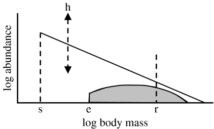
Relationships between abundance and body mass were used to describe the structure of consumer communities and to calculate their biomass, production and trophic level. This approach captures the main features of strongly size-structured marine food webs, where body mass rather than species identity accounts for the main patterns of energy flux. Building on the theory that links the slopes of relationships between log abundance and log body mass (size spectra) to transfer efficiency (ϵ) and the predator–prey mass ratio (μ; Brown et al. 2004), we predicted the slope and intercept of a size spectrum leading from the median phytoplankton body mass class to the largest consumers (figure 1).

Figure 1.

Schematic of the process used to predict total animal biomass and teleost or elasmobranch biomass in each grid cell. The height (h) of the size spectrum and the smallest size class (s) in the spectrum are functions of PP (which affect phytoplankton biomass and size composition). Teleosts or elasmobranchs (shaded area) are assumed to be part of total community of animals larger than the size of their eggs or live young (e) and their biomass in all size classes is predicted in relation to an assumed biomass in a given size class (r).

The slope of the size spectrum was used to determine B in larger body mass classes. Slope was calculated as $W^{(\text{log}ϵ/\text{log}\mu )+0.25}$, an approach that has been validated empirically at a regional scale (Jennings & Mackinson 2003). We assumed log μ=3 (e.g. Cushing 1975; Boudreau & Dickie 1992) and ϵ=0.125 (e.g. Ware 2000), but conducted sensitivity analyses to assess the effects of assumptions about μ and ϵ on biomass and production estimates. The relationship between trophic level and body mass was also defined by the value of μ, since an increase in consumer mass of μ corresponded to an increase of one in trophic level. Phytoplankton, at the base of the food chain, were assigned a trophic level of one.

(d) Biomass and production of animal groups based on life history

To explore how the biomass and production of specific groups might be distinguished from total biomass and production (figure 1), we considered the example of marine groups with differing life histories: teleost fish and elasmobranchs (sharks and rays). These groups are distinguished by their size at birth or hatch and their potential maximum size, the latter being correlated with growth rate (e.g. Hoenig & Gruber 1990).

We assumed that each group had a generalized life history, recruiting to the size spectrum as eggs or live young and leaving the spectrum when mortality had reduced adult numbers to zero. Following recruitment, the relationship between mortality and growth determines biomass and, in the steady state, mortality M=P in any body mass class. To determine the contribution of groups to total biomass in each body mass class, we assumed that mortality rates were constant at body mass but that faster growth through a body mass class would reduce realized mortality. The mean residence time of an individual in a body mass class was thus approximated as

$$t=\frac{W_{\text{u}}-W_{\text{l}}}{P_{\text{u}}+P_{\text{l}}},$$ (2.4)

where W_u and W_l are the upper and lower body mass limits in the class and P_u and P_l are the corresponding upper and lower limits for individual production. During period t, the mean instantaneous rate of mortality M can be approximated as

$$M=0.5(M_{\text{u}}+M_{\text{l}}),$$ (2.5)

where M_u and M_l are the values of M at the upper and lower body mass limits in the class. The effects of body mass and temperature on mortality were estimated by rearranging the equation of Brown et al. (2004)

$$M=\text{exp}(c_1-E/kT)W^{-0.24},$$ (2.6)

where c₁ is a constant. Brown et al. (2004) fit this equation to estimates of M for populations, but we assume that the same scaling applies to a combination of individuals and populations.

On average, species with larger asymptotic sizes are larger at any given age than species with smaller asymptotic sizes (Hoenig & Gruber 1990) and mortality rates fall with body size (e.g. Duplisea 2005). Mortality in a body mass class was assumed to fall if an animal grew more rapidly through the class, though this simplifies the outcome of a more complex trade-off where faster growth is also associated with an increase in mortality after accounting for the effects of body mass (Gislason et al. in press). To describe differences in the growth rates through body mass classes, a simple multiplier (c₂) was used to modify t, where

$$c_2=1-((\alpha -W_{\text{m}})\beta ),$$ (2.7)

where α is the W at which c₂t=t and β modifies the rate at which c₂t increases or decreases in relation to t as W increases or decreases in relation to α. The change in numbers of animals with increasing body mass class can now be expressed as

$$N_{W_{\text{m}}+1}=N_W\text{exp}(-M{c}_{2}t).$$ (2.8)

Equations (2.7) and (2.8) were applied to teleosts and elasmobranchs. For teleosts, fish were assumed to be present in all body mass classes more than or equal to 10^−3.05 g (assume that all teleosts begin life as an egg with a mean diameter of 1–1.5 mm). In class 10^0.05 g (midpoint 1.1 g), we assumed that fishes of all species would have recruited but that no fishes would have reached their asymptotic mass. These assumptions were based on reported egg sizes for marine fish (Chambers 1997) and an analysis of the frequency distributions of the maximum body masses of fishes in large marine ecosystems which showed that a very small proportion of species have a maximum body mass less than 1 g (see electronic supplementary material). We assumed that 50% of individuals in class 10^0.05 g were fish, providing the initial value of N for forward and back-calculation of N at W. This was an approximation and the real value would be expected to vary among regions and over time (see electronic supplementary material). The value of α was set as 2.95 and β as 0.05, to satisfy this condition.

For elasmobranchs, we assessed biomass and production for coastal and oceanic species, where coastal species were defined as those inhabiting depths less than or equal to 200 m. This distinction was based on differences in the life history and distribution of these groups. Oceanic epipelagic species living away from shelf areas but typically at depths less than 200 m (Compagno in press) were assumed to be present in all body mass classes greater than or equal to 10^3.55 (consistent with a mean size at birth=3258 g±2.6 g 95% CI, n=15, data from Goodwin et al. 2002). It was assumed that oceanic epipelagic elasmobranchs accounted for 20% of numbers in body mass class 10^4.05 (midpoint=11 220 g) and that all species would be present in this class. Given fishing effects in contemporary marine ecosystems, this was necessarily an approximation (see electronic supplementary material). The value of α was set as 5.75 and β as 0.2. Coastal elasmobranchs that live on shelves to 200 m depth are smaller at birth (mean=221 g±1.3 g 95% CI n=167, data from Goodwin et al. 2002) and were allocated to all classes greater than 10^2.35. They were assumed to account for 10% of numbers in class 10^2.95. The value of α was set to 4.75 and β as 0.2 to satisfy this condition. The percentage contributions of pelagic and coastal elasmobranchs to abundance at size are only approximations because there are few data to assess their potential role in ecosystems, given their vulnerability to fishing and negligible data on community composition in the absence of fishing (Friedlander & DeMartini 2002). Elasmobranchs living at depths more than 200 m (oceanic mesopelagic and slope species) were not considered in the analysis owing to their very low abundance and productivity (Merrett & Haedrich 1997).

To balance M and P, c₂ in equation (2.6) was set to make the slopes based on energy availability and on the P and M trade-offs identical. For ϵ=0.125 and μ=3, the value of c₂ was 26.001 compared with 26.25 when the model was fitted to data (Brown et al. 2004).

Trophic levels of teleosts and elasmobranchs were calculated in relation to the trophic level (λ) at the midpoint of the phytoplankton size range, which was defined as

$${\lambda }_{W_{\text{mp}}}=\frac{(B_{\text{p}}{\lambda }_{\text{p}})+(B_{\text{z}}{\lambda }_{\text{z}})}{(B_{\text{p}}+B_{\text{z}})},$$ (2.9)

where B_p and B_z are the biomass density of phytoplankton and zooplankton, respectively. For λ_p=1 and λ_z=2 and assuming ϵ=0.125, ${\lambda }_{W_{\text{mp}}}$=1.11. Given that log μ=3, the trophic level of any given body mass (${\lambda }_{W_{\text{m}}}$) will be

$${\lambda }_{W_{\text{m}}}={\lambda }_{W_{\text{mp}}}+\left[\frac{(\text{log}W-\text{log}{W}_{\text{mp}})}{3}\right].$$ (2.10)

Further details of the methods and assumptions are provided in the electronic supplementary material.

3. Results

By linking concepts from macroecology, life-history theory and food-web ecology, PP and temperature data could be used to predict the biomass and production of marine animals on a global scale. Production of all animals could be estimated for 90% of the total ocean area (3.21×10⁸ km² of the 3.57×10⁸ km² that could be allocated to FAO fishing areas, see electronic supplementary material). Total PP in this area was 4.1×10¹¹ tonnes wet weight yr⁻¹, equivalent to 1204 g m⁻² yr⁻¹.

The estimated global biomass of all animals more than 10⁻⁵ g wet weight was 2.62×10⁹ t (=8.16 g m⁻² ocean), and these animals had a production of 1.00×10¹⁰ t (31.15 g m⁻²; table 1). Production fell much faster than biomass with increasing body mass, for animals weighing more than 1 g, biomass was 1.02×10⁹ t (2.95 g m⁻², 39% of total) while production was 3.45×10⁸ t yr⁻¹ (1.00 g m⁻² y⁻¹, 3.4% of total).

Table 1.

Potential global marine animal biomass and production by body mass, expressed as wet weight.

body mass	biomass (B)			production (P)
g	106 t	g m−2	percentage of total	106 t yr−1	g m−2 yr−1	percentage of total
10−5–10−4	400.67	1.25	15	4893.16	15.22	49
10−4–10−3	356.25	1.11	14	2503.57	7.79	25
10−3–10−2	316.76	0.99	12	1280.94	3.99	13
10−2–10−1	281.64	0.88	11	655.39	2.04	7
10−1–100	250.42	0.78	10	335.33	1.04	3
100–101	222.66	0.69	8	171.57	0.53	2
101–102	197.97	0.62	8	87.78	0.27	1
102–103	176.03	0.55	7	44.91	0.14	<1
103–104	156.51	0.49	6	22.98	0.07	<1
104–105	139.16	0.43	5	11.76	0.04	<1
105–106	123.73	0.38	5	6.02	0.02	<1
totals	2621.81	8.16	100	10 013.40	31.15	100

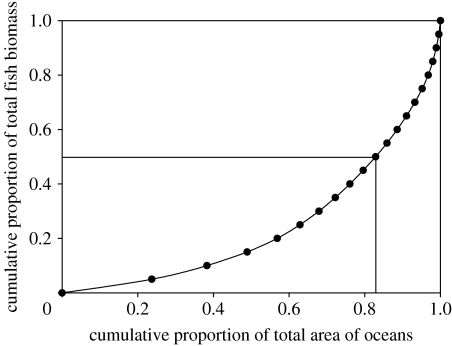
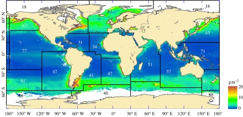
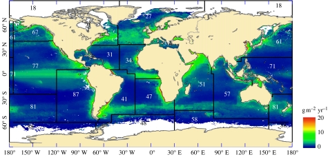
Global fish biomass was approximated as 8.99×10⁸ t (2.80 g m⁻²) and annual production as 7.91×10⁸ t yr⁻¹ (2.46 g m⁻²; table 2). Fifty per cent of teleost biomass occurs in 17% of the total area of the oceans (figure 2), corresponding to an average biomass of 8.22 g m⁻², while 25% of teleost biomass occurs in only 5% of the ocean (14.0 g m⁻²). The areas with high teleost biomass and production are predominantly the upwellings and coastal shelves in mid latitudes (figures 3 and 4). The contribution of elasmobranchs to total fish biomass was estimated to be 0.86×10⁷ t, equivalent to 0.27 g m⁻², while annual production was much lower at 0.06×10⁸ t yr⁻¹ (0.02 g m⁻²; table 2).

Table 2.

Potential global fish biomass and production by body mass. (FB, fish biomass (teleosts and elasmobranchs); FP, fish production; EB, elasmobranch biomass; EP, elasmobranch production expressed as wet weight; TB, teleost biomass.)

body mass	FB			FB			EB			EP			FB/AB	TB/(TB+EB)
g	106 t	g m−2	percentage of total	106 t	g m−2 yr−1	percentage of total	106 t	g m−2	percentage of total	106 t	g m−2 yr−1	percentage of total	%	%
10−5–10−4	—	—	0	—	—	0	—	—	0	—	—	0	0	0
10−4–10−3	11.01	0.03	1	62.55	0.19	8	—	—	0	—	—	0	3	100
10−3–10−2	51.76	0.16	6	203.68	0.63	26	—	—	0	—	—	0	16	100
10−2–10−1	78.43	0.24	9	178.61	0.56	23	—	—	0	—	—	0	28	100
10−1–100	104.95	0.33	12	138.33	0.43	17	—	—	0	—	—	0	42	100
100–101	123.31	0.38	14	94.11	0.29	12	—	—	0	—	—	0	55	100
101–102	127.08	0.40	14	56.13	0.17	7	—	—	0	—	—	0	64	100
102–103	115.91	0.36	13	29.61	0.09	4	0.25	0.00	<1	0.05	0.00	1	66	100
103–104	106.26	0.33	12	15.46	0.05	2	13.31	0.04	15	1.71	0.01	26	68	87
104–105	100.61	0.31	11	8.52	0.03	1	34.65	0.11	40	2.87	0.01	44	72	66
105–106	79.38	0.25	9	3.91	0.01	<1	38.05	0.12	44	1.86	0.01	29	64	52
totals	898.70	2.80	100	790.90	2.46	100	86.26	0.27	100	6.49	0.02	100	34	90

Figure 2.

Relationship between the cumulative biomass of teleost fishes and the area of ocean where the biomass is found. The horizontal and vertical lines denote the area of ocean occupied by 50% of total biomass.

Figure 3.

The distribution of teleost biomass. The overlays show the FAO fishing areas and their corresponding codes (see electronic supplementary material for further details). PP estimates were not available for the areas shown in white.

Figure 4.

The distribution of teleost production. The overlays show the FAO fishing areas and their corresponding codes (see electronic supplementary material for further details).

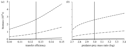
Sensitivity analyses illustrated that variations in transfer efficiency and predator–prey mass ratios within expected bounds could influence the global biomass estimate for all animals by approximately 3.5-fold and for teleosts and elasmobranchs by 5- and 7-fold, respectively (figure 5). The effects of the same variation in these parameters on the biomass and production of the different animal groups, in different size classes and at different temperatures, were typically greater than the effects on total biomass and production, since the selected groups had higher than average trophic level (see electronic supplementary material). Changes to the exponent in the P and W relationship (equation (2.2)) by ±0.4 from the assumed value of 0.76 changed the total global biomass estimate of all animals (and fish) by less than threefold. The range 0.72–0.80 was large in relation to reported 95% CI for fitted W exponents. For example, Brown et al. (2004) report 0.75–0.76 for the exponent in equation (2.2). While these narrow CI reflect the wide range in body mass over which the relationships were fitted, we also applied the exponents over as many as 17 orders of magnitude in body mass (see electronic supplementary material). We consider that errors in biomass estimates associated with probable variation in scaling exponents will be small in relation to those attributable to plausible changes in predator–prey mass ratio or transfer efficiency.

Figure 5.

Sensitivity of global biomass estimates to the assumed (a) transfer efficiency and (b) predator–prey mass ratio. Dashed lines represent all biomass, dash-dotted lines represent teleost biomass and solid lines represent elasmobranch biomass. The vertical lines pass through the values of ϵ and log μ used in the main analysis. Additional sensitivity analyses are provided in the electronic supplementary material.

Fish comprised more than 50% of all marine animals in size classes weighing more than 1 g (table 2). While most (more than 50%) fish production was attributed to animals weighing less than 1 g, the bulk of biomass was in fish weighing more than 10 g. The total biomass of fish of 10 g and upwards, which are most likely to be taken in fisheries, was 5.29×10⁸ t (1.65 g m⁻²) and production was 1.14×10⁸ t yr⁻¹ (0.35 g m⁻² yr⁻¹), giving a production to biomass ratio of 0.22 (table 2). All the elasmobranch biomass (0.27 g m⁻²) and production (0.02 g m⁻² yr⁻¹) is in size classes likely to be available to fisheries. Fish biomass accounted for 34% of the total biomass of animals weighing more than 10⁻⁵ g (table 2).

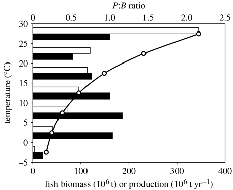
The production of all animals weighing more than 10⁻⁵ g per unit area was the highest at 10–15°C, but biomass was the highest at 0–5°C. Fish biomass per unit area was the highest at 0–5°C and more than five times that in the warm area (6.58 versus 1.22 g m⁻²). Fish production per unit area was the highest at 10–15°C (3.32 g m⁻²) but less than a quarter of this in polar regions less than 0°C. The fish production to biomass ratios is more than 10 times higher at greater than 25°C than at less than 5°C (figure 6; see electronic supplementary material). Total fish production was the highest in areas where sea surface temperature was greater than 25°C and total biomass was the highest in areas where the temperature was 5–10°C (figure 6). However, sea surface temperatures are greater than 25°C over more than 38% of the global ocean and thus the mean production per unit area (2.62 g m⁻²) at greater than 25°C is not so high as at intermediate (10–20°C) temperatures.

Figure 6.

Total fish biomass (black bars) and production (white bars) as a function of sea surface temperature (°C). The open circles show changes in the mean production (P) to biomass (B) ratio of the fish community with temperature.

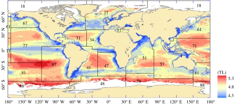
Production to biomass ratios for elasmobranchs indicated the low potential productivity of these large species, even at higher temperatures. The ratio of PP to fish production and elasmobranch production tended to be lower at intermediate temperatures, reflecting the association between these temperatures and relatively high PP (see electronic supplementary material). The mean trophic level of fishes was highest in the ocean gyres where picoplankton were predicted to be more abundant and PP was low, giving rise to longer food chains (figure 7; see electronic supplementary material). There were large regional variations in fish biomass and production, with lower production to biomass ratios associated with the cooler areas in higher latitudes (see electronic supplementary material for production and biomass estimates by FAO area and temperature).

Figure 7.

Spatial variation in the mean trophic level of the fish community. The overlays show the FAO fishing areas and their corresponding codes (see electronic supplementary material for further details).

4. Discussion

Our analysis is based on simple relationships between body size, energy acquisition and transfer that account for much of the variation in the structure and function of communities (e.g. Dickie et al. 1987; Gaston & Blackburn 2000; Brown et al. 2004; Hildrew et al. 2007). Since these relationships and their interaction with temperature are common to many biological systems, we expect that our approach can be developed to assess the role of changing climatic temperature and PP on production at higher trophic levels (Sarmiento et al. 2004) and to set baselines for assessing the impacts of fisheries (Jennings & Blanchard 2004) that appropriate a significant proportion of production in the marine environment (Pauly & Christensen 1995). One benefit of our approach is that it uses remote sensing temperature and PP data, available on global scales, to predict properties of marine communities in environments that are challenging and expensive to sample directly. For example, knowledge of the distribution and abundance of some of the most abundant pelagic fish, such as species of Myctophidae, is extremely limited, despite their potentially significant role in food webs and biogeochemical processes (Huntley et al. 1991). An additional benefit of our approach is that the predictions of biomass and production are size structured, which is important if model outputs were to be used to estimate rates and fluxes that scale with body size. Our simple approach will not replace sophisticated and parameter hungry models for assessing climate or fishing effects on individual species at a regional scale (e.g. Brander et al. 2001), but can complement such models in the many other areas where the data available for parametrization are inadequate or the models do not focus on processes that are common to all marine systems.

Our estimates of biomass and production are most likely to be accurate for the open oceans in mid and low latitudes, where estimates of PP based on ocean colour data are considered to be more accurate (Gregg & Casey 2007), where phytoplankton dominate PP (Duarte & Cebrián 1996) and where the rate of loss of pelagic production to the sea floor is relatively low (Dunne et al. 2005). The open oceans are also the areas for which production and biomass estimates of fauna are the least reliable, and the contribution of some groups, such as myctophid fishes, is poorly known. Our estimates are likely to be less accurate in inshore areas, where estimates of PP based on ocean colour data may be less accurate, where groups other than phytoplankton contribute to total production and where export is greater (Dunne et al. 2005). In addition, when using our method to estimate potential fish production, we note that contemporary rates of PP may be influenced by the nutrient removal that occurs when fish are caught. The sensitivity analyses demonstrate that outputs were sensitive to assumptions about transfer efficiency and predator–prey mass ratios. However, the effects of errors in the estimated parameters are unlikely to be compounded since relationships between transfer efficiency and predator–prey mass ratios are expected to be compensatory (e.g. Brown & Gillooly 2003).

The temporal sampling of ocean colour is increasingly irregular at higher latitudes owing to cloud cover and high solar zenith angles. As a result, the conditions when the ocean surface can be sampled in high latitudes correspond with periods of low cloud cover and/or low zenith angles; conditions that also promote phytoplankton blooms. This often leads to overestimation of PP in regions where remote sensing coverage is poor (Gregg & Casey 2007). For this reason, we did not attempt to extrapolate from the few records we have in high latitude areas and our estimate of global fish and animal production applies to 90% of the area of the global ocean.

A number of assumptions were made in our analyses. These were that (i) phytoplankton production supports all other production, (ii) phytoplankton production supports production at higher trophic levels in the same grid cell, (iii) surface temperatures reflect the temperature experience of the biota in the water column, (iv) all predation and energy transfer is size based, (v) the proportion of fish and elasmobranchs in at least one (unfished) size class is known, (vi) all teleosts and elasmobranchs enter the size spectrum in a single body mass class, and (vii) a simple relationship between growth rate and mortality adequately captures changes in abundance of teleosts and elasmobranchs with size. Our justifications for these assumptions and their potential effects on our conclusions are discussed in the electronic supplementary material. The main limitation of our analysis was the absence of an approach for rigorously predicting the relative contributions of teleost or elasmobranch biomass to total biomass when data were sparse and fishing has modified contemporary food webs. The development of theory that predicts the relative dominance of animal groups at body mass from their life history is likely to be the most promising way to rectify this deficiency.

At regional scales, variations in PP can account for a significant proportion of the variance in fish production (Iverson 1990; Frank et al. 2006). Our estimate of potential global fish production of 7.91×10⁸ t is more than three times that predicted by Ryther (1969). He assumed that PP was 2×10¹⁰ t C yr⁻¹, less than half the values more recently reported by Longhurst et al. (1995) and Carr et al. (2006). Differences between our fish production estimate and that of Ryther (1969) probably result from the higher total PP assumed in our analysis, our focus on all size classes of fish and our finer resolution of the factors affecting food chain length.

Mean teleost biomass was predicted to be 8.22 g m⁻² in 17% of ocean area, principally upwellings and productive shelf areas. Fish catches in heavily fished areas of productive shelf such as the Georges Bank and North Sea can range from 1.5 to 6.7 g m⁻² yr⁻¹ (Sparholt 1990), and Frank et al. (2006) reported catches of 0.59–2.70 g m⁻² in a series of fishing grounds off the east coast of North America (Labrador Shelf to the Grand Bank). The lower, but not the higher reported catch rates, are broadly consistent with our biomass estimates and knowledge of compensatory responses to fishing mortality. These responses suggest that annual yield is usually sustainable when biomass is reduced to approximately 60% of the unexploited biomass and when annual catches are equivalent to 20–40% of the reduced biomass (e.g. Hilborn & Walters 1992). The higher catch rates suggest that we may have underestimated fish biomass in these inshore areas where non-phytoplankton sources contribute to PP, or that the reported catch rates are sustained by PP that is drawn from a wider area than the fishing grounds where catches were recorded. The model also underestimated known teleost production in the Humboldt current, but less so for the other Eastern Boundary Currents (see electronic supplementary material).

We conclude that theoretical developments in metabolic ecology, macroecology, allometry, life-history theory and food-web ecology can be combined to formulate simple models for predicting the potential biomass, production, size structure and trophic structure of consumer communities. Our application demonstrates that emerging ecological theory can be synthesized to address applied problems on a global scale, since the outputs provide baselines for assessing the relative impacts of humans and predicting the global contribution of marine animals to biogeochemical processes.

Supplementary Material

JMBFDW PRSB ESM 2008

File containing all ESM

References

- Agawin N.S.R, Duarte C.M, Agusti S. Nutrient and temperature control of the contribution of picoplankton to phytoplankton biomass and production. Limnol. Oceanogr. 2000;45:591–600. [Google Scholar]
- Boudreau P.R, Dickie L.M. Biomass spectra of aquatic ecosystems in relation to fisheries yield. Can. J. Fish. Aquat. Sci. 1992;49:1528–1538. [Google Scholar]
- Brander K.M, Dickson R.R, Shepherd J.G. Modelling the timing of plankton production and its effect on recruitment of cod (Gadus morhua) ICES J. Mar. Sci. 2001;58:962–966. doi:10.1006/jmsc.2001.1086 [Google Scholar]
- Brown J.H. University of Chicago Press; Chicago, IL: 1995. Macroecology; p. 269. [Google Scholar]
- Brown J.H, Gillooly J.F. Ecological food webs: high-quality data facilitate theoretical unification. Proc. Natl Acad. Sci. USA. 2003;100:1467–1468. doi: 10.1073/pnas.0630310100. doi:10.1073/pnas.0630310100 [DOI] [PMC free article] [PubMed] [Google Scholar]
- Brown J.H, Gillooly J.F, Allen A.P, Savage V.M, West G.B. Towards a metabolic theory of ecology. Ecology. 2004;85:1771–1789. doi:10.1890/03-9000 [Google Scholar]
- Carr M.-E, et al. A comparison of global estimates of marine primary production from ocean color. Deep-Sea Res. II. 2006;53:741–770. doi:10.1016/j.dsr2.2006.01.028 [Google Scholar]
- Chambers R.C. Environmental influences on egg and propagule sizes in marine fishes. In: Chambers R.C, Trippel E.A, editors. Early life history and recruitment in fish populations. Chapman & Hall; London, UK: 1997. pp. 63–102. [Google Scholar]
- Compagno, L. J. V. In press. Pelagic sharks definition. In Sharks of the open ocean: biology, fisheries and conservation (eds M. A. Camhi & E. K. Pikitch). Oxford, UK: Blackwell Science.
- Cushing D.H. Cambridge University Press; Cambridge, UK: 1975. Marine ecology and fisheries. [Google Scholar]
- Dickie L.M, Kerr S.R, Boudreau P.R. Size-dependent processes underlying regularities in ecosystem structure. Ecol. Monogr. 1987;57:233–250. doi:10.2307/2937082 [Google Scholar]
- Duarte C.M, Cebrián J. The fate of marine autotrophic production. Limnol. Oceanogr. 1996;41:1758–1766. [Google Scholar]
- Dunne J.P, Armstrong R.A, Gnnadesikan A, Sarmiento J.L. Empirical and mechanistic models for the particle export ratio. Glob. Biogeochem. Cycles. 2005;19:GB4026. doi:10.1029/2004GB002390 [Google Scholar]
- Duplisea D.E. Running the gauntlet: the predation environment of small fish in the northern Gulf of St Lawrence, Canada. ICES J. Mar. Sci. 2005;62:412–416. doi:10.1016/j.icesjms.2004.11.005 [Google Scholar]
- Ernest S.K.M, et al. Thermodynamic and metabolic effects on the scaling of production and population energy use. Ecol. Lett. 2003;6:990–995. doi:10.1046/j.1461-0248.2003.00526.x [Google Scholar]
- Frank K.T, Petrie B, Shackell N.L, Choi J.S. Reconciling differences in trophic control in mid-latitude marine ecosystems. Ecol. Lett. 2006;9:1–10. doi: 10.1111/j.1461-0248.2006.00961.x. doi:10.1111/j.1461-0248.2006.00961.x [DOI] [PubMed] [Google Scholar]
- Friedlander A.M, DeMartini E.D. Contrasts in density, size and biomass of reef fishes between the northwestern and the main Hawaiian islands: the effects of fishing down apex pedators. Mar. Ecol. Progress Ser. 2002:253–264. doi:10.3354/meps230253 [Google Scholar]
- Gaston K.J, Blackburn T.M. Blackwell Science; Oxford, UK: 2000. Pattern and process in macroecology. [Google Scholar]
- Gislason H, Pope J.G, Rice J, Daan N. Coexistence in marine fish communities—implications for growth and natural mortality. ICES J. Mar. Sci. 2008;65:514–530. doi:10.1093/icesjms/fsn035 [Google Scholar]
- Goodwin N.B, Dulvy N.K, Reynolds J.D. Life history correlates of the evolution of live-bearing in fishes. Phil. Trans. R. Soc. B. 2002;357:259–267. doi: 10.1098/rstb.2001.0958. doi:10.1098/rstb.2001.0958 [DOI] [PMC free article] [PubMed] [Google Scholar]
- Gregg W.W, Casey N.W. Sampling biases in Modis and SeaWiFS ocean chlorophyll data. Remote Sens. Environ. 2007;111:25–35. doi:10.1016/j.rse.2007.03.008 [Google Scholar]
- Hilborn R, Walters C.J. Chapman and Hall; New York, NY: 1992. Quantitative fisheries stock assessment: choice, dynamics and uncertaincy. [Google Scholar]
- Hildrew A.G, Raffaelli D.G, Edmonds-Bown R, editors. Body size: the structure and function of aquatic ecosystems. Cambridge University Press; Cambridge, UK: 2007. [Google Scholar]
- Hoenig, J. M. & Gruber, S. H. 1990 Life-history patterns in the elasmobranchs: implications for fisheries management. NOAA techincal report NMFS no. 90. pp. 1–16.
- Huntley M.E, Lopez M.D.G, Karl D.M. Top predators in the southern ocean: a major leak in the biological carbon pump. Science. 1991;253:64–66. doi: 10.1126/science.1905841. doi:10.1126/science.1905841 [DOI] [PubMed] [Google Scholar]
- Iverson R.L. Control of marine fish production. Limnol. Oceanogr. 1990;35:1593–1604. [Google Scholar]
- Jennings S, Blanchard J.L. Fish abundance with no fishing: predictions based on macroecological theory. J. Anim Ecol. 2004;73:632–642. doi:10.1111/j.0021-8790.2004.00839.x [Google Scholar]
- Jennings S, Mackinson S. Abundance–body mass relationships in size structured food webs. Ecol. Lett. 2003;6:971–974. doi:10.1046/j.1461-0248.2003.00529.x [Google Scholar]
- Kerr S.R, Dickie L.M. Columbia University Press; New York, NY: 2001. The biomass spectrum: a predator–prey theory of aquatic production. [Google Scholar]
- Li W.K.W. Macroecological patterns of phytoplankton in the northwestern Atlantic Ocean. Nature. 2002;419:154–157. doi: 10.1038/nature00994. doi:10.1038/nature00994 [DOI] [PubMed] [Google Scholar]
- Longhurst A, Sathyendranath S, Platt T, Caverhill C. An estimate of global primary production in the ocean from satellite radiometer data. J. Plankton Res. 1995;17:1245–1271. doi:10.1093/plankt/17.6.1245 [Google Scholar]
- McClain C.R, Feldman G.C, Hooker S.B. An overview of the SeaWiFS project and strategies for producing a climate research quality global ocean bio-optical time series. Deep-Sea Res. II. 2004;51:5–42. doi:10.1016/j.dsr2.2003.11.001 [Google Scholar]
- Merrett N.R, Haedrich R.L. Chapman and Hall; London, UK: 1997. Deep-sea demersal fish and fisheries. [Google Scholar]
- Pauly D, Christensen V. Primary production required to sustain global fisheries. Nature. 1995;374:255–257. doi:10.1038/374255a0 [Google Scholar]
- Ryther J.H. Relationships of photosynthesis to fish production in the sea. Science. 1969;166:72–76. doi: 10.1126/science.166.3901.72. doi:10.1126/science.166.3901.72 [DOI] [PubMed] [Google Scholar]
- Sarmiento J.L, et al. Response of ocean ecosystems to climate warming. Glob. Biogeochem. Cycles. 2004;18:1–23. doi:10.1029/2003GB002134 [Google Scholar]
- Sheldon R, Parsons T. A continuous size spectrum for particulate matter in the sea. J. Fish. Res. Board Can. 1967;24:909–915. [Google Scholar]
- Sparholt H. An estimate of the total biomass of fish in the North Sea. Journal du Conseil, Conseil– International pour l'Exploration de la Mer. 1990;46:200–210. [Google Scholar]
- Ware D.M. Aquatic ecosystems: properties and models. In: Harrison P.J, Parsons T.R, editors. Fisheries oceanography: an integrative approach to fisheries ecology and management. Blackwell Science; Oxford, UK: 2000. pp. 161–194. [Google Scholar]
Associated Data
This section collects any data citations, data availability statements, or supplementary materials included in this article.
Supplementary Materials