Bayesian Template Estimation in Computational Anatomy

Abstract

Templates play a fundamental role in Computational Anatomy. In this paper, we present a Bayesian model for template estimation. It is assumed that observed images I₁, I₂, …, I_N are generated by shooting the template J through Gaussian distributed random initial momenta θ₁, θ₂, …, θ_N. The template J is modeled as a deformation from a given hypertemplate J₀ with initial momentum μ, which has a gaussian prior. We apply a mode approximation of the EM (MAEM) procedure, where the conditional expectation is replaced by a Dirac measure at the mode. This leads us to an image matching problem with a Jacobian weight term, and we solve it by deriving the weighted Euler-Lagrange equation. The results of template estimation for hippocampus and cardiac data are presented.

1 Introduction

Computational Anatomy (CA) is the mathematical study of variability of anatomical and biological shapes. The framework has been pioneered by Grenander [11] through the notion of deformable templates. Given a template I_temp, the group of diffeomorphisms 𝒢 acts on it to generate an orbit ℐ = 𝒢.I_temp, a whole family of new objects with similar structure as I_temp. Hence, one can model elements in the orbit ℐ via diffeomorphic transformations.

Templates play an important role in CA. They are usually used to generate digital anatomical atlases and act as a reference when computing shape variability. Often, templates have been chosen to be manually selected “typical” observed images. It is however preferable to build a template based on statistical properties of the observed population. There has been by now several publications addressing the issue of shape averaging over a dataset. In this context, the average is based on metric properties of the space of shapes; assuming a distance in shape space is given, the average of a set of shapes is a minimizer of the sum of square distances to each element of the set (Fréchet or Karcher mean). When the shape space is modeled as a Riemannian manifold, a local minimum of this sum of squared distances must be such that the sum of initial velocities of the geodesics between the average and each of the elements in the set vanishes. This leads to the following averaging procedure (sometimes called procrustean averaging) which consists in (i)starting with an initial guess of the average, (ii) computing all the geodesics between this current average and each element in the set of shapes, (iii) averaging their initial velocities and (iv) displacing the current average to the endpoint of the geodesic starting with the initial velocity, this being iterated until convergence [12, 20, 9, 16, 21]. A different variational definition of the average has been provided in [15, 5, 4]. In the present work, however, we do not build the template as a metric average, but as the central component of a generative statistical model for the anatomy. This is reminiscent of the construction developed in [1] for linear models of deformations, and in [10] for thin-plate models of points set.

In our application of Grenander’s pattern theory, anatomical shapes are modeled as an orbit under the action of the group of diffeomorphisms. Because of this, diffeomorphisms play an important role in our statistical model. The nonlinear space of diffeomorphisms can be studied as an infinite dimensional Riemannian manifold, on which, with a suitable choice of metric, geodesic equations are described by a momentum conservation law [2, 3, 14, 17]. In our context, the methodology of geodesic shooting [23, 19] relies on this conservation law to derive statistical models on diffeomorphisms and deformable objects. Through the geodesic equations, the flow at any point along the geodesic is completely determined (once a template is fixed) by the momentum at the origin. The initial momentum therefore provides a linear representation of the nonlinear diffeomorphic shape space in a local chart around the template, to which linear statistical analysis can be applied. Note that metric averaging can be reconnected to geodesic shooting [23, 13]. In this case, the algorithm is: first, compute the geodesic from a given template I₀ to several target images and obtain the initial momenta of each transformations; second, compute the mean initial momentum m̄; then, shoot I₀ with initial momentum m̄ to get a new image Ī; iterate this procedure. This approach was used in landmark matching [23], 3D average digital atlas construction [6] and quantifying variability in heart geometry [13].

In this paper, we introduce a random statistical model on the initial momentum to represent random deformations of a template. The generative model we use combines this deformation with some observation noise. We will then develop a strategy to estimate the template from observations, based on a mode approximation of the EM algorithm (MAEM), under a Bayesian framework.

The paper is organized as follows. We first provide some background material and notation related to diffeomorphisms and their use in computational anatomy. We then discuss template estimation and detail the statistical model and the implementation of the MAEM procedure. This will require in particular introducing an extension of the LDDMM algorithm [7, 18] to the case where the data attachment term has a nonstationary spatial weight. We finally provide experimental results, with a comparison with a simplified, non-bayesian, approach.

1.1 Background

Let the background space Ω ⊂ ℝ^d be a bounded domain on which the images are defined. To a template I_temp corresponds the orbit ℐ = {I_temp ∘ g⁻¹ : g ∈ 𝒢} under the group of diffeormorphisms 𝒢. For any two anatomical images J, I ∈ ℐ, there exists a set of diffeomorphisms (denote g as an arbitrary element in the set) that registers the given images: I = J ∘ g⁻¹. Following [8, 22], when we define the orbit ℐ, we restrict to diffeomorphisms that can be generated as flows g_t, t ∈ [0, 1] controlled by a velocity field υ_t, with the relation

$$\frac{\partial g_t}{\partial t}\left(x\right)={\upsilon }_t\left(g_t\left(x\right)\right),x\in \mathrm{\Omega },t\in \left[0,1\right]$$ (1)

with initial condition g₀ = id. To ensure that the ODEs generate diffeomorphisms, the vector fields are constrained to be sufficiently smooth [8, 22]. More specifically, they are assumed to belong to (V, ‖·‖_V ), a Hilbert space with squared norm defined as ‖υ‖_V = (Aυ, υ) through an operator A : V ↦ V*, where V* is the dual space of V . For υ ∈ V , Aυ can be considered as a linear form on V (a mapping from V to ℝ) through the identification (Aυ,w) = 〈υ,w〉_V, where (Aυ,w) is the standard notation for a linear form Aυ applied to w. Interpreting ${\Vert \upsilon \Vert }_V^2=\left(A\upsilon ,\upsilon \right)$ as an energy, Aυ will be called the momentum associated to the velocity υ. We assume that V can be embedded in a space of smooth functions, which makes it a reproducing kernel Hilbert space with kernel K = A⁻¹ : V* ↦ V .

The geodesics in the group of diffeomorphisms are time-dependent diffeomorphisms t ↦ g_t defined by (1) such that the integrated energy

$${\displaystyle {\int }_0^1{\Vert {\upsilon }_t\Vert }_V^{2}dt}$$ (2)

is minimal with fixed boundary conditions g₀ and g₁. The image matching problem between J and I is formalized as the search for the optimal geodesic starting at g₀ = id such that $I=J\circ g_1^{-1}$. From this is derived the inexact matching problem, which consists in finding a time-dependent vector field υ_t solution of the problem

$$\widehat{\upsilon }=\underset{\upsilon :{\mathit{ġ}}_t={\upsilon }_t\left(g_t\right)}{\text{argmin}}\left({\displaystyle {\int }_0^1{\Vert {\upsilon }_t\Vert }_V^2\mathrm{d}t}+\frac{1}{{\sigma }^2}{\Vert J\circ g_1^{-1}-I\Vert }_2^2\right).$$ (3)

Geodesics are characterized by the following Euler equation (sometimes called EPDiff [14]), which can be interpreted as a conservation equation for the momentum Aυ [2, 3]. The equation is

$$\frac{\partial A{\upsilon }_t}{\partial t}+{\left(D{\upsilon }_t\right)}^{*}A{\upsilon }_t+\text{div}\left({\upsilon }_t\right)A{\upsilon }_t+D\left(A{\upsilon }_t\right){\upsilon }_t=0.$$ (4)

The conservation of momentum is described as follows. Let w₀ be a vector field, and $w_t=D{g}_t(g_t^{-1})w_0(g_t^{-1})$ be the transported vector field along the geodesic. Then, if Aυ_t satisfies Eq. (4), we have:

$$\frac{\partial }{\partial t}(A{\upsilon }_t,w_t)=0.$$ (5)

This implies $A{\upsilon }_t={(D{g}_t^{-1})}^{*}A{\upsilon }_0(g_t^{-1})|D{g}_t^{-1}|,t\in [0,1]$, meaning that the geodesic evolution in the orbit $J\circ g_t^{-1}$ depends only on J and the momentum at time 0. The solution of (3) satisfies this property in an even simpler form, which explicitly provides the momentum Aυ_t in function of the deformed images and the diffeomorphism g_t [7, 18]. Moreover, Eq. (5) can be shown to have singular solutions that propagate over time. In fluid mechanics, EPDiff is used to model the propagation of waves on shallow water. In our context, it provides a very simple form to finitely generate models of deformation (see section 3.2).

Hence, the nonlinear diffeomorphic shapes can be represented by the initial momenta which lie on a linear space (the dual of V ). This provides a powerful vehicle for statistical analysis of shapes. In this paper, we investigate a statistical model of deformable template estimation using this property.

Note that, if υ̂, with associated diffeomorphism ĝ, is a (local) minimum of (3), it is also a (local) minimum of the problem:

$$\underset{\upsilon :{\mathit{ġ}}_t={\upsilon }_t\left(g_t\right),g_1={\widehat{g}}_1}{\text{argmin}}\left({\displaystyle {\int }_0^1{\Vert {\upsilon }_t\Vert }_V^2\mathrm{d}t}\right).$$ (6)

since the data term in (3) only depends on g₁. Therefore (since (6) is equivalent to the geodesic minimization on groups of diffeomorphisms), υ̂ satisfies the EPDiff equation, which is therefore also relevant for inexact matching (as noticed in [19]).

2 Methodology of Template Estimation

2.1 Statistical model for the anatomy

In addition to the conservation of momentum discussed in the previous section, solutions of (3) have also their energy conserved (since they are geodesics): ${\Vert {\upsilon }_t\Vert }_V^2$ is independent of time. Because of this, problem (3) is equivalent to

$$\widehat{\upsilon }=\underset{\upsilon :{\mathit{ġ}}_t={\upsilon }_t\left(g_t\right)}{\text{argmin}}\left({\Vert {\upsilon }_0\Vert }_V^2+\frac{1}{{\sigma }^2}{\Vert J\circ g_1^{-1}-I\Vert }_2^2\right).$$ (7)

where υ₀ is the initial velocity. So the minimization is now restricted to time-dependent vector fields υ that satisfy (4). The minimized expression may formally be interpreted as a joint log-likelihood for the initial velocity υ₀ and observed image I in which υ₀ would be a random field (with V as a reproducing space) generating, via (4), a diffeomorphism g₁, and I would be obtained from the deformed template by the addition of a white noise.

This is essentially the model we adopt in this paper, under a discrete form that will be more amenable to rigorous computation. Recall that we have defined the duality operator A on V as associating to υ in V the linear form Aυ ∈ V* defined by (Aυ,w) = 〈υ,w〉_V . By the Riesz representation theorem, A is invertible with inverse A⁻¹ = K. The discretization will be done on the momentum, m = Aυ, instead of the velocity field υ.

Note that the sets V and V* are isometric if V* is equipped with the product 〈m,m̃〉_V* = (m, Km̃) for m, m̃ ∈ V*. Therefore, the norm of initial velocity is equal to the norm of corresponding initial momentum, that is, for m₀ = Aυ₀, we have

$$\left(A{\upsilon }_0,{\upsilon }_0\right)={\Vert {\upsilon }_0\Vert }_V^2={\Vert m_0\Vert }_{V^{*}}^2=\left(m_0,K{m}_0\right).$$ (8)

Formally again, this may be interpreted as the log-likelihood of a Gaussian distribution on V* with covariance operator A = K⁻¹, characterized by the property that, for any w ∈ V , (m₀,w) is a centered Gaussian distribution with variance

$$E\left\{{\left(m_0,w\right)}^2\right\}=\left(Aw,w\right)={\Vert w\Vert }_V^2.$$ (9)

We now discuss a discrete version of this random field. For x, a ∈ ℝ^d, denote a ⊙ δ_x the linear form w ↦ (a ⊙ δ_x,w) ≔ a^Tw(x). Noting that K(a ⊙ δ_x) ∈ V is, by definition, a vector field on V that depends linearly on a, we make the abuse of notation

$$K\left(a\odot {\delta }_x\right)\left(y\right)=K\left(y,x\right)a$$

where K(y, x) is a d by d matrix (the reproducing kernel of V ). It can be checked that K(x, y) = K(y, x)^T and

$${\langle K\left(·,y\right)a,K\left(·,z\right)b\rangle }_V=a^{T}K(y,z)b.$$

We model the random momentum θ as a sum of such measures

$$\theta ={\displaystyle \sum _{i=1}^S{a}_i\odot {\delta }_{x_i}}$$ (10)

where x₁, x₂, …, x_S ∈ Ω form a set of fixed (deterministic) points (for example, the grid supporting the image discretization) and a = (a₁, a₂, …, a_S) are random variables such that a ~ 𝒩(0,∑) in ℝ^Sd. We want to choose ∑ consistently with our formal interpretation of Eq.(8). For this, we can compute, for w ∈ V

$$\left(\theta ,w\right)={\displaystyle \sum _{i=1}^S{a}_i^{T}w\left(x_i\right)}$$ (11)

which is a Gaussian with mean 0 and variance

$${\displaystyle \sum _{i,j=1}^{S}w{\left(x_i\right)}^T{\sum }_{ij}w\left(x_j\right)}$$

where ∑_ij is the d by d matrix $E(a_i{a}_j^T)$. We want to compare this to equation (9), and in particular ensure that both expressions coincide when w = K(·, x_k)b for some b ∈ ℝ^d and k ∈ {1,…, S}. In this case, we have ${\Vert w\Vert }_V^2=b^{T}K\left(x_k,x_k\right)b$ yielding the constraint: for all k

$$K\left(x_k,x_k\right)={\displaystyle \sum _{i,j=1}^{S}K\left(x_k,x_i\right){\sum }_{ij}K\left(x_j,x_k\right)}.$$

Define K̃_ij = K(x_i, x_j) and assume that the block matrix K̃ = (K̃_ij) is invertible. Then the equation above is equivalent to ∑ = K̃⁻¹, which completely describes the distribution of (a₁,…, a_S).

The probability density function (p.d.f) of a is given by

$$p(a)=\frac{1}{Z}{e}^{-\frac{1}{2}{a}^T{\sum }^{-1}a}=\frac{1}{Z}{e}^{-\frac{1}{2}{a}^T\mathit{K̃}a}$$ (12)

where $Z={\left(2\pi \right)}^{Sd/2}/\sqrt{\text{det}\mathit{K̃}}$.

It is interesting to notice that we have, with $\theta ={\displaystyle {\sum }_{i=1}^S{a}_i\odot {\delta }_{x_i}}$,

$$\begin{array}{cc}\left(\theta ,K\theta \right)\hfill & ={\displaystyle \sum _{i,j=1}^S(a_i\odot {\delta }_{x_i},K\left(·,x_j\right)a_j)}\hfill \\ \hfill & ={\displaystyle \sum _{i,j=1}^S{a}_i^{T}K\left(x_i,x_j\right)a_j}\hfill \end{array}$$ (13)

$$=a^T\mathit{K̃}a.$$ (14)

So the p.d.f of θ can be written as

$$p(\theta )=\frac{1}{Z}{e}^{-\frac{1}{2}\left(\theta ,K\theta \right)}{\mathbf{1}}_{V^{*}\left(x\right)}\left(\theta \right)$$ (15)

where 1 represents the indicator function and $V^{*}\left(x\right)=\left\{\theta ={\displaystyle {\sum }_{i=1}^S{a}_i\odot {\delta }_{x_i},a_1,\dots ,a_S\in {ℝ}^d}\right\}$. Since in the infinite dimensional space V*, our model is a singular Gaussian distribution supported by the finite dimensional space V*(x). When restricted on this space, it is continuous with respect to the Lebesgue measure with a density provided by Eq. (15).

This describes the deformation part of the model, represented as the distribution of the initial momentum θ. We can solve (4) with initial condition Aυ₀ = θ from time t = 0 to t = 1 and integrate the velocity field t ↦ υ_t to obtain a diffeomorphism, that we shall denote g_θ, at time t = 1. Although we will not use this fact in our numerical methods, it is important to notice that g_θ can be obtained from θ (given by Eq. (10)) via the solution of a system of ordinary differential equations to which Eq. (4) reduces. It can be shown that this system has solutions over all times, so our model is theoretically consistent. With this model, the image $J\circ g_{\theta }^{-1}$is therefore a random deformation of the template (since θ is random). We assume that the observed image I obtained from the deformed template after discretization and addition of noise. More precisely, denoting $[J\circ g_{\theta }^{-1}]={\displaystyle {\sum }_{i=1}^S{\delta }_{x_i}J\circ g_{\theta }^{-1}}$, the observation I is a discrete image given by

$$I=\left[J\circ g_{\theta }^{-1}\right]+W,W\sim 𝒩\left(0,{\sigma }^{2}Id\right).$$ (16)

The complete process is thus via the pair (θ, I). Our goal is, given observations I₁, …, I_N having the same distribution as I above, to estimate the template J and the noise variance σ².

2.2 Prior distribution on the template

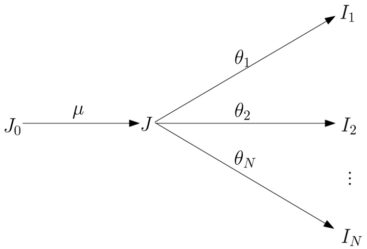
We want to constrain the virtually infinite dimensional template estimation problem within a Bayesian strategy. We will introduce for this a hypertemplate, J₀, and describe J as a random deformation of J₀. The hypertemplate is given, usually provided by an anatomical atlas. The template J is modeled as $J=J_0\circ g_{\mu }^{-1}$ with μ the initial momentum. We model μ as a discrete momentum like in the previous section, with distribution

$$\pi (\mu )=\frac{1}{Z_{\pi }}{e}^{-\frac{1}{2}\left(\mu ,K_{\pi }\mu \right)}{\mathbf{1}}_{V^{*}\left(x\right)}\left(\mu \right)$$ (17)

for a reproducing kernel K_π. In our experiments, we made the simple choice K_π = λK, for some regularization parameter λ > 0.

The relations between J₀,J and I₁, I₂, …, I_N is illustrated in Figure 1.

Figure 1.

The template J is to be estimated given hypertemplate J₀ and observed images I₁, I₂, …, I_N. We model the template as $J=J_0\circ g_{\mu }^{-1}$, where μ is the random initial momentum. In the following EM algorithm, μ is computed iteratively, with random initial momenta θ₁, θ₂, …, θ_N being hidden variables.

Remark

In this model, J₀ and J are continuous. J₀ is a given continuous function defined on Ω ∈ ℝ^d, although it may be finitely generated (using a finite element representation, for example). Observations I₁, …, I_N are discrete images. From these images, we will estimate the initial momentum μ, and further get the continuous template $J=J_0\circ g_{\mu }^{-1}$. For simplicity, we will still denote, with a little abuse, $J\circ g_{{\theta }_n}^{-1}$ to refer to its discretization $[J\circ g_{{\theta }_n}^{-1}]$.

Remark

The kernels K and K_π are important components of the model, and can be considered as infinite dimensional parameters. While not an impossible task, trying to estimate them would significantly complicate our procedure. Consequently, the kernels have been selected a priori, and left fixed during the estimation procedure.

3 Template Estimation with the MAEM Algorithm

3.1 The complete-data log-likelihood

We here describe the estimation of parameters μ (which uniquely describes the template) and σ² based on the observation of I = {I₁, I₂,…, I_N}. Our goal is to compute argmax_μ,σ² p_σ(μ|I). We let Θ = {θ₁, θ₂, …, θ_N} denote the sequence of hidden initial momenta.

To use the EM algorithm we first write down the complete-data log-likelihood. The joint likelihood of the model given the observations is

$$\begin{array}{cc}\hfill & p\left(\mu ,\mathbf{I},\mathrm{\Theta }\right)=\pi \left(\mu \right)p\left(\mathbf{I},\mathrm{\Theta }|\mu \right)\hfill \\ =\hfill & \frac{1}{Z_{\pi }}{e}^{-\frac{1}{2}\left(\mu ,K_{\pi }\mu \right)}{\displaystyle \prod _{n=1}^N\frac{1}{Z}{e}^{-\frac{1}{2}\left({\theta }_n,K{\theta }_n\right)-\frac{1}{2{\sigma }^2}{\Vert J_0\circ g_{\mu }^{-1}\circ g_{{\theta }_n}^{-1}-I_n\Vert }_2^2-\frac{1}{2}S\text{log}{\sigma }^2}}\hfill \end{array}$$ (18)

Where ${\Vert I-\mathit{I\prime }\Vert }_2^2={{\displaystyle {\sum }_{i=1}^S\left(I\left(x_i\right)-\mathit{I\prime }\left(x_i\right)\right)}}^2$.

The EM algorithm generates a sequence (μ^(k), σ^2(k)) according to the transition (E_{μ^(k),σ^2(k)} is the expectation under the assumption that the true parameters are μ^(k) and σ^2(k).)

$$({\mu }^{\left(k+1\right)},{\sigma }^{2\left(k+1\right)})=\underset{\mu ,{\sigma }^2}{\text{argmax}}{E}_{{\mu }^{\left(k\right)},{\sigma }^{2\left(k\right)}}\left(\text{log}{p}_{\sigma }\left(\mu ,\mathbf{I},\mathbf{\Theta }\right)|\mathbf{I}\right).$$

The maximization is decomposed into two steps implying a generalized EM algorithm:

$${\sigma }^{2\left(k+1\right)}=\underset{{\sigma }^2}{\text{argmax}}{E}_{{\mu }^{\left(k\right)},{\sigma }^{2\left(k\right)}}\left(\text{log}{p}_{\sigma }\left(\mu ,\mathbf{I},\mathbf{\Theta }\right)|\mathbf{I}\right)$$

$${\mu }^{\left(k+1\right)}=\underset{\mu }{\text{argmax}}{E}_{{\mu }^{\left(k\right)},{\sigma }^{2\left(k+1\right)}}\left(\text{log}{p}_{\sigma }\left(\mu ,\mathbf{I},\mathbf{\Theta }\right)|\mathbf{I}\right).$$

Define the complete-data log-likelihood Q(μ, σ²|μ^(k), σ^2(k), I) as the right hand side of the previous equation which must be maximized alternatively in μ and σ²:

$$\begin{array}{c}Q(\mu ,{\sigma }^2|{\mu }^{\left(k\right)},{\sigma }^{2\left(k\right)},\mathbf{I})\hfill \\ =E_{{\mu }^{\left(k\right)}}\{-\frac{1}{2}\left(\mu ,K_{\pi }\mu \right)\hfill \\ -{\displaystyle \sum _{n=1}^N\frac{1}{2}\left({\theta }_n,K{\theta }_n\right)-\frac{1}{2{\sigma }^2}{\displaystyle \sum _{n=1}^N{\Vert J_0\circ g_{\mu }^{-1}\circ g_{{\theta }_n}^{-1}-I_n\Vert }_2^2-\frac{NS}{2}\text{log}{\sigma }^2|\mathbf{I}\}}+C}\hfill \\ =-\frac{1}{2}\left(\mu ,K_{\pi }\mu \right)\hfill \\ -\frac{1}{2{\sigma }^2}{\displaystyle \sum _{n=1}^N{E}_{{\mu }^{\left(k\right)}}\left\{{\Vert J_0\circ g_{\mu }^{-1}\circ g_{{\theta }_n}^{-1}-I_n\Vert }_2^2{I}_n\right\}-\frac{NS}{2}\text{log}{\sigma }^2}+\mathit{C̃}\hfill \end{array}$$ (19)

where S is the number of grids (or pixels, voxels) and C and C̃ are expressions that do not depend on μ or σ². The maximization M-step at transition step k yields

$${\sigma }^{2\left(k+1\right)}=\frac{1}{SN}{\displaystyle \sum _{n=1}^N{E}_{{\mu }^{\left(k\right)}}\left\{{\Vert J_0\circ g_{{\mu }^{\left(k\right)}}^{-1}\circ g_{{\theta }_n}^{-1}-I_n\Vert }_2^2|I_n\right\}}$$ (20)

$$\begin{array}{cc}{\mu }^{(k+1)}=\hfill & \underset{\mu }{\text{argmin}}\{\left(\mu ,K_{\pi }\mu \right)\hfill \\ \hfill & +\frac{1}{{\sigma }^{2\left(k+1\right)}}{\displaystyle \sum _{n=1}^N{E}_{{\mu }^{\left(k\right)}}{\{\Vert J_0\circ g_{\mu }^{-1}\circ g_{{\theta }_n}^{-1}-I_n\Vert }_2^2\left|I_n\}\right\}}\hfill \end{array}$$ (21)

Remark

The resulting MAEM algorithm formally coincides with the Maximum a Posterior (MAP) estimation, which maximizes the likelihood with respect to all parameters. We use MAEM here instead of MAP to be reminded that the deformation (with respect to which the mode is computed) is not a parameter, but a hidden variable, and that our procedure should be considered as an approximation of the computation of the maximum likelihood of the observations.

3.2 Maximization via the Euler Equation with Jacobian weight

This is the EM framework for template estimation. Now, the main difficulty of the algorithm is the minimization in (21). To derive the Euler -Lagrange Equation for the minimizer, we use the integral formula for the norm, so we can avoid the interpolation problem associated with discrete sum definition ${\Vert I-\mathit{I\prime }\Vert }_2^2={{\displaystyle {\sum }_{i=1}^S\left(I\left(x_i\right)-\mathit{I\prime }\left(x_i\right)\right)}}^2$ which corresponds to signal plus additive white noise. This makes the change of variable formula straightforward and links us to the Euler-Lagrange equations on vector fields which have been previously published. As well, our implementation is a discretization of that continuum equation. Note that one can provide a fully discrete analysis of the problem (relying on a representation of the images using linear interpolations as in [1], where both images and deformations are linear combinations of the kernels centered at the landmark points. ).

For the variation, let V_π be the reproducing kernel Hilbert space associated to the prior kernel K_π. Since the energy is conserved along geodesics, we have

$$\left(\mu ,K_{\pi }\mu \right)={\Vert {\upsilon }_0\Vert }_{V_{\pi }}^2={\displaystyle {\int }_0^1{\Vert {\upsilon }_t\Vert }_{V_{\pi }}^2\mathrm{d}t}$$ (22)

where υ₀ = K_πμ is the initial velocity. This connects our optimization in the MAEM algorithm to the original LDDMM Euler-Lagrange equation of [7].

If g_t is a time-dependent flow of diffeomorphisms, we let g_s,t : Ω ↦ Ω denote the composition g_s,t(y) = g_t ∘ (g_s)⁻¹(y), meaning position at time t of a particle that is at position y at time s. Let Dg_s,t denote the Jacobian of mapping g_s,t, the matrix composed with the space derivatives. We add a superscript υ to indicate that $g_t=g_t^{\upsilon }$ is the flow arising from (1). We state how perturbations of the vector field affect the variation of the mapping in the following lemma.

Lemma 3.1

The variation of mapping $g_{s,t}^{\upsilon }$ when υ ∈ L²([0, 1], V_π) is per-turbed along h ∈ L²([0, 1], V_π) is given by

$${\partial }_h{g}_{s,t}^{\upsilon }=\underset{\epsilon \to 0}{\text{lim}}\frac{g_{s,t}^{\upsilon +\epsilon h}-g_{s,t}^{\upsilon }}{\epsilon }=D{g}_{s,t}^{\upsilon }{\displaystyle {\int }_t^s{(D{g}_{s,u}^{\upsilon })}^{-1}{h}_u\circ g_{s,u}^{\upsilon }}\mathrm{d}u.$$ (23)

Refer to [7] for proof.

Then the maximization is reduced to what we term the weighted-LDDMM image matching problem.

Proposition 3.1

(i) (Formalization to a weighted-LDDMM problem) At stage k + 1 define the following ancillary average of the conditional mean:

$${\mathit{Ī}}^{(k+1)}\left(y\right)=\frac{{\displaystyle {\sum }_{n=1}^N{E}_{{\mu }^{(k)}}\{I_n\circ g_{{\theta }_n}(y)|D{g}_{{\theta }_n}(y)||I_n\}}}{{\displaystyle {\sum }_{n=1}^N{E}_{{\mu }^{(k)}}\{|D{g}_{{\theta }_n}(y)||I_n\}}}.$$ (24)

Then the M-step of the generalized EM algorithm reduces to the weighted-LDDMM algorithm:

$$\begin{array}{cc}{\mu }^{(k+1)}\hfill & =\underset{\mu }{\text{argmin}}\{(\mu ,K_{\pi }\mu )\hfill \\ \hfill & +{\displaystyle \sum _{n=1}^N\frac{1}{{\sigma }^{2(k+1)}}{E}_{{\mu }^{(k)}}\{{\Vert J_0\circ g_{\mu }^{-1}\circ g_{{\theta }_n}^{-1}-I_n\Vert }_2^2|I_n\}\}}\hfill \\ \hfill & =\underset{\mu }{\text{argmin}}\{(\mu ,K_{\pi }\mu )+\frac{1}{{\sigma }^{2(k+1)}}{\displaystyle {\int }_{\mathrm{\Omega }}{(J\circ g_{\mu }^{-1}(y)-{\mathit{Ī}}^{(k+1)}(y))}^2{\alpha }^{(k+1)}(y)\mathrm{d}y\}}\hfill \end{array}$$ (25)

with the Jacobian weight

$${\alpha }^{\left(k+1\right)}\left(y\right)={\displaystyle \sum _{n=1}^N{E}_{{\mu }^{\left(k\right)}}\left\{|D{g}_{{\theta }_n}\left(y\right)||I_n\right\}.}$$ (26)

(ii) (The weighted Euler-Lagrange Equation) Given a continuously differentiable template image J₀, a target image Ī and Jacobian weight α, the optimal velocity field υ̂ ∈ L²[(0, 1), V_π] with υ̂₀ = K_πμ̂ for inexact matching of J₀ and Ī defined as

$$\underset{\upsilon :{\mathit{ġ}}_t={\upsilon }_t\left(g_t\right)}{\text{argmin}}\left\{{\displaystyle {\int }_0^1{\Vert {\upsilon }_t\Vert }_{V_{\pi }}^{2}dt}+\frac{1}{{\sigma }^2}{\displaystyle {\int }_{\mathrm{\Omega }}{(\mathit{Ī}\left(y\right)-J_0\circ g_{\mu }^{-1}\left(y\right))}^2\alpha \left(y\right)\mathrm{d}y}\right\}$$ (27)

satisfies the Euler-Lagrange equation

$$2{\widehat{\upsilon }}_t-K_{\pi }\left(\frac{2}{{\sigma }^2}|D{g}_{t,1}|\nabla H_t^0(H_t^0-H_t^1)\alpha \circ g_{t,1}\right)=0$$ (28)

where $H_t^0=J_0\circ g_{t,0},H_t^1=\mathit{Ī}\circ g_{t,1}$.

The crucial idea here is that we are linked back to the basic LDDMM image matching problem of Beg (α = 0), with the Jacobian playing a role.

Proof

(i)Let $y=g_{{\theta }_n}^{-1}\left(x\right)$, we have

$$\begin{array}{cc}\hfill & {\Vert J_0\circ g_{\mu }^{-1}\circ g_{{\theta }_n}^{-1}-I_n\Vert }_2^2\hfill \\ \approx \hfill & {\displaystyle {\int }_{\mathrm{\Omega }}{(J_0\circ g_{\mu }^{-1}\circ g_{{\theta }_n}^{-1}\left(x\right)-I_n\left(x\right))}^2\mathrm{d}x}\hfill \\ =\hfill & {\displaystyle {\int }_{\mathrm{\Omega }}{(J_0\circ g_{\mu }^{-1}\left(y\right)-I_n\circ g_{{\theta }_n}\left(y\right))}^2|D{g}_{{\theta }_n}\left(y\right)|\mathrm{d}y}\hfill \end{array}$$ (29)

With Ī^(k+1) as defined in Eq. 24, we have, for all y ∈ Ω

$$\begin{array}{cc}\hfill & {\displaystyle \sum _{n=1}^N{E}_{{\mu }^{\left(k\right)}}\{{(J_0\circ g_{\mu }^{-1}\left(y\right)-I_n\circ g_{{\theta }_n}\left(y\right))}^2|D{g}_{{\theta }_n}\left(y\right)||I_n\}}\hfill \\ =\hfill & {\displaystyle \sum _{n=1}^N{E}_{{\mu }^{\left(k\right)}}\{(J_0\circ g_{\mu }^{-1}\left(y\right)-{\mathit{Ī}}^{\left(k+1\right)}\left(y\right)}\hfill \\ \hfill & +{\mathit{Ī}}^{\left(k+1\right)}\left(y\right)-I_n\circ g_{{\theta }_n}{\left(y\right))}^2|D{g}_{{\theta }_n}\left(y\right)||I_n\}\hfill \\ =\hfill & {\displaystyle \sum _{n=1}^N{E}_{{\mu }^{\left(k\right)}}\{{(J_0\circ g_{\mu }^{-1}\left(y\right)-{\mathit{Ī}}^{\left(k+1\right)}\left(y\right))}^2|D{g}_{{\theta }_n}\left(y\right)|}\hfill \\ \hfill & +({\mathit{Ī}}^{\left(k+1\right)}\left(y\right)-I_n\circ g_{{\theta }_n}{\left(y\right))}^2|D{g}_{{\theta }_n}\left(y\right)|\hfill \\ \hfill & +2(J_0\circ g_{\mu }^{-1}(y)-{\mathit{Ī}}^{\left(k+1\right)}\left(y\right))({\mathit{Ī}}^{\left(k+1\right)}\left(y\right)\hfill \\ \hfill & -I_n\circ g_{{\theta }_n}\left(y\right))|D{g}_{{\theta }_n}\left(y\right)||I_n\}\hfill \\ {=}^{\left(a\right)}\hfill & {\displaystyle \sum _{n=1}^N{E}_{{\mu }^{\left(k\right)}}\{{(J_0\circ g_{\mu }^{-1}\left(y\right)-{\mathit{Ī}}^{\left(k+1\right)}\left(y\right))}^2|D{g}_{{\theta }_n}\left(y\right)|}\hfill \\ \hfill & +({\mathit{Ī}}^{\left(k+1\right)}\left(y\right)-I_n\circ g_{{\theta }_n}{\left(y\right))}^2|D{g}_{{\theta }_n}\left(y\right)||I_n\}\hfill \\ =\hfill & {(J_0\circ g_{\mu }^{-1}\left(y\right)-{\mathit{Ī}}^{\left(k+1\right)}\left(y\right))}^2{\displaystyle \sum _{n=1}^N{E}_{{\mu }^{\left(k\right)}}\{|D{g}_{{\theta }_n}\left(y\right)||I_n\}}\hfill \\ \hfill & +{\displaystyle \sum _{n=1}^N{E}_{{\mu }^{\left(k\right)}}\{{\mathit{Ī}}^{\left(k+1\right)}\left(y\right)-I_n\circ g_{{\theta }_n}{\left(y\right))}^2|D{g}_{{\theta }_n}\left(y\right)||I_n\}}.\hfill \end{array}$$ (30)

In (a), the fact that the cross item

$$\begin{array}{cc}\hfill & {\displaystyle \sum _{n=1}^N{E}_{{\mu }^{(k)}}\{(J_0\circ g_{\mu }^{-1}(y)}\hfill \\ \hfill & -{\mathit{Ī}}^{(k+1)}(y))({\mathit{Ī}}^{(k+1)}(y)-I_n\circ g_{{\theta }_n}(y))|D{g}_{{\theta }_n}(y)||I_n\}\hfill \\ =\hfill & (J_0\circ g_{\mu }^{-1}(y)-{\mathit{Ī}}^{(k+1)}(y)){\displaystyle \sum _{n=1}^N{E}_{{\mu }^{(k)}}\{({\mathit{Ī}}^{(k+1)}(y)}\hfill \\ \hfill & -I_n\circ g_{{\theta }_n}(y))|D{g}_{{\theta }_n}(y)||I_n\}=0\hfill \end{array}$$

comes straightforward from the definition of Ī^(k+1)(y).

Since the second term of Eq.(30) does not depend on μ, substituting Eq. (30) into Eq. (21), we see that μ^(k+1) must minimize

$$\left(\mu ,K_{\pi }\mu \right)+\frac{1}{{\sigma }^{2\left(k+1\right)}}{\displaystyle {\int }_{\mathrm{\Omega }}{({\mathit{Ī}}^{\left(k+1\right)}\left(y\right)-J_0\circ g_{\mu }^{-1}\left(y\right))}^2{\alpha }^{\left(k+1\right)}\left(y\right)\mathrm{d}y}$$ (31)

with the Jacobian weight

$${\alpha }^{\left(k+1\right)}\left(y\right)={\displaystyle \sum _{n=1}^N{E}_{{\mu }^{\left(k\right)}}\{|D{g}_{{\theta }_n}\left(y\right)|}|I_n\}$$ (32)

. With the optimal μ^(k+1), we can compute g_μ^(k+1) by geodesic shooting (Equation (4)), and further obtain the newly estimated template $J^{\left(k+1\right)}=J_0\circ g_{{\mu }^{\left(k+1\right)}}^{-1}$. This gives the first part of the proof.

(ii)The proof of the second half follows the derivation in [7]. Suppose the velocity υ ∈ L²([0, 1], V_π) is perturbed along the direction h ∈ L²[(0, 1), V_π] by an ε amount. The Gâteaux variation ∂_hE(υ) of the energy function is expressed in term of the Fréchet derivative ∇_υE

$${\partial }_{h}E\left(\upsilon \right)=\underset{\epsilon \to 0}{\text{lim}}\frac{E\left(\upsilon +\epsilon h\right)-E\left(\upsilon \right)}{\epsilon }={\displaystyle {\int }_0^1{\langle {\nabla }_{\upsilon }{E}_t,h_t\rangle }_{V_{\pi }}}\mathrm{d}t.$$ (33)

The variatio n of $E_1(\upsilon )={\displaystyle {\int }_0^1{\Vert {\upsilon }_t\Vert }_{V_{\pi }}^2}\mathrm{d}t$ is given by

$${\partial }_h{E}_1\left(\upsilon \right)=2{\displaystyle {\int }_0^1{\langle {\upsilon }_t,h_t\rangle }_{V_{\pi }}}\mathrm{d}t.$$ (34)

The second part of the energy is

$$\begin{array}{cc}{E}_2\left(\upsilon \right)\hfill & =\frac{1}{{\sigma }^2}{\displaystyle {\int }_{\mathrm{\Omega }}{(J_0\circ g_1^{-1}\left(y\right)-\mathit{Ī}\left(y\right))}^2\alpha \left(y\right)\mathrm{d}y}\hfill \\ \hfill & =\frac{1}{{\sigma }^2}{\langle (J_0\circ g_{1,0}-\mathit{Ī})\alpha ,J_0\circ g_{1,0}-\mathit{Ī}\rangle }_{L^2}.\hfill \end{array}$$ (35)

The variation of E₂(υ) is

$$\begin{array}{cc}{\partial }_h{E}_2\left(\upsilon \right)\hfill & =\frac{2}{{\sigma }^2}{\langle (J_0\circ g_{1,0}-\mathit{Ī})\alpha ,D{J}_0\circ g_{1,0}{\partial }_h{g}_{1,0}\rangle }_{L^2}\hfill \\ \hfill & {=}^{\left(a\right)}\frac{2}{{\sigma }^2}{\langle (J_0\circ g_{1,0}-\mathit{Ī})\alpha ,D{J}_0\circ g_{1,0}\left(-D{g}_{1,0}{\displaystyle {\int }_0^1{\left(D{g}_{1,t}\right)}^{-1}{h}_t\circ g_{1,t}}\mathrm{d}t\right)\rangle }_{L^2}\hfill \\ \hfill & {=}^{\left(b\right)}-\frac{2}{{\sigma }^2}{\displaystyle {\int }_0^1{\langle (J_0\circ g_{1,0}-\mathit{Ī})\alpha ,D\left(J_0\circ g_{1,0}\right){\left(D{g}_{1,t}\right)}^{-1}{h}_t\circ g_{1,t}\rangle }_{L^2}\mathrm{d}t}\hfill \end{array}$$ (36)

with (a) derived straightly from Lemma 3.1 and (b) from the formulation D(J₀ ∘ g_1,0) = DJ₀ ∘ g_1,0Dg_1,0. Changing variable with z = g_1,t(y) i.e. g_t,1(z) = y, one can obtain |dg_t,1| dz = dy. The chain rule gives g_1,0 ∘ g_t,1 = g_t,0. In addition, D(I ∘ g) = (∇(I ∘ g))^T . With these substitutions, we get

$$\begin{array}{ccc}{\partial }_h{E}_2\left(\upsilon \right)\hfill & =\hfill & -\frac{2}{{\sigma }^2}{\displaystyle {\int }_0^1{\langle |D{g}_{t,1}|\left(J_0\circ g_{t,0}-\mathit{Ī}\circ g_{t,1}\right)\alpha \circ g_{t,1},D\left(J_0\circ g_{t,0}\right)h_t\rangle }_{L^2}\mathrm{d}t}\hfill \\ \hfill & =\hfill & -\frac{2}{{\sigma }^2}{\displaystyle {\int }_0^1{\langle |D{g}_{t,1}|\nabla \left(J_0\circ g_{t,0}\right)\left(J_0\circ g_{t,0}-\mathit{Ī}\circ g_{t,1}\right)\alpha \circ g_{t,1},h_t\rangle }_{L^2}\mathrm{d}t}\hfill \\ \hfill & =\hfill & -{\displaystyle {\int }_0^1{\langle K_{\pi }\left(\frac{2}{{\sigma }^2}|D{g}_{t,1}|\nabla \left(J_0\circ g_{t,0}\right)\left(J_0\circ g_{t,0}-\mathit{Ī}\circ g_{t,1}\right)\alpha \circ g_{t,1}\right),h_t\rangle }_{V_{\pi }}\mathrm{d}t}\hfill \\ \hfill & =\hfill & -{\displaystyle {\int }_0^1{\langle K_{\pi }\left(\frac{2}{{\sigma }^2}|D{g}_{t,1}|\nabla H_t^0(H_t^0-H_t^1)\alpha \circ g_{t,1}\right),h_t\rangle }_{V_{\pi }}\mathrm{d}t.}\hfill \end{array}$$

Combining the two parts of energy functional, the gradient is thus

$${\left({\nabla }_{\upsilon }{E}_t\right)}_{V\pi }=2{\upsilon }_t-K_{\pi }\left(\frac{2}{{\sigma }^2}|D{g}_{t,1}|\nabla H_t^0(H_t^0-H_t^1)\alpha \circ g_{t,1}\right)$$ (37)

where the subscript V_π in (∇_υE_t)_Vπ is to clarify that the gradient is in the space L²([0, 1], V_π). The optimizing velocity fields satisfy the Euler-Lagrange equation

$${\nabla }_{h}E\left(\widehat{\upsilon }\right)={\displaystyle {\int }_0^1{\langle 2{\widehat{\upsilon }}_t-K_{\pi }\left(\frac{2}{{\sigma }^2}|D{g}_{t,1}|\nabla H_t^0(H_t^0-H_t^1)\alpha \circ g_{t,1}\right),h_t\rangle }_{V\pi }}\mathrm{d}t=0.$$ (38)

Since h is arbitrary in L²([0, 1], V_π) we get Eq.(28).

Equation (37) provides the gradient flow that minimizes (27). Recall that this problem must be solved to obtain the next deformation of the hypertemplate: given the solution υ̂, compute the initial momentum μ̂ = (K_π)⁻¹υ̂₀, the optimal diffeomorphism g_μ̂ and the new template $J=J_0\circ g_{\widehat{\mu }}^{-1}$.

Since the Euler-Lagrange equation for theWeighted LDDMM only differs from the original equation by the α∘g_t,1 factor, its implementation is a minor modification to the basic one, for which we refer to [7] for details.

3.3 Computing the conditional mean via the mode

Another difficulty is to compute the conditional expectations, which cannot be done analytically, given the highly nonlinear relation between θ_n and I_n ∘ g_θn. The crudest approximation of the conditional distribution is to replace it by a Dirac measure at its mode, and this is the one we will select for the time being. Already having J^(k), estimation of the template in k-th iteration, denote ${\theta }_n^{\left(k\right)}$ to be the minimizer of

$$\left({\theta }_n,K{\theta }_n\right)+\frac{1}{{\sigma }^{2\left(k\right)}}{\Vert J^{\left(k\right)}\circ g_{{\theta }_n}^{-1}-I_n\Vert }_2^2.$$ (39)

The computation of Ī^(k+1) now becomes:

$${\mathit{Ī}}^{\left(k+1\right)}\left(y\right)=\frac{{\displaystyle {\sum }_{n=1}^N{I}_n\circ g_{{\theta }_n^{\left(k\right)}}\left(y\right)|D{g}_{{\theta }_n^{\left(k\right)}}\left(y\right)|}}{{\displaystyle {\sum }_{n=1}^N|D{g}_{{\theta }_n^{\left(k\right)}}\left(y\right)|}}.$$ (40)

This also provides an approximation of the Jacobian weight

$${\alpha }^{\left(k+1\right)}\left(y\right)={\displaystyle \sum _{n=1}^N|D{g}_{{\theta }_n^{\left(k\right)}}\left(y\right)|.}$$ (41)

Concerning the implementation, the computation of ${\theta }_n^{\left(k\right)}$is done using the LDDMM algorithm between the template J^(k) and the target I_n. Note that ${\theta }_n^{\left(k\right)}$ is not needed for Eq. (40), but only the deformed target $I_n\circ g_{{\theta }_n^{\left(k\right)}}$ and the determinant of the Jacobian $D{g}_{{\theta }_n^{\left(k\right)}}$.

3.4 Template Estimation Algorithm

Now, the template estimation algorithm can be summarized as the following:

Algorithm 3.1 (Template estimation)

Having the hypertemplate J₀ and N observations I₁, I₂, …, I_N, we wish to estimate the template J and noise variance σ². Let J^(k) denote the estimated template after k iterations with initial guess J⁽⁰⁾ = J₀. Then, the (k + 1)th step is

(i) Map the current estimated template J^(k) to I_n, n = 1, 2, …,N using basic LDDMM, and obtain the deformed targets $I_n\circ g_{{\theta }_n^{\left(k\right)}}$ and Jacobian determinants of the deformations $|D{g}_{{\theta }_n^{\left(k\right)}}|$.

(ii) Compute the mean image Ī^(k+1) and the Jacobian weight α^(k+1) defined by

$${\mathit{Ī}}^{\left(k+1\right)}\left(y\right)=\frac{{\displaystyle {\sum }_{n=1}^N{I}_n\circ g_{{\theta }_n^{\left(k\right)}}\left(y\right)|D{g}_{{\theta }_n^{\left(k\right)}}\left(y\right)|}}{{\displaystyle {\sum }_{n=1}^N|D{g}_{{\theta }_n^{\left(k\right)}}\left(y\right)|}},$$ (42)

and

$${\alpha }^{\left(k+1\right)}\left(y\right)={\displaystyle \sum _{n=1}^N|D{g}_{{\theta }_n^{\left(k\right)}}\left(y\right)|}$$ (43)

where $g_{{\theta }_n^{(k)}}$ is the optimal diffeomorphic mapping from J^(k) to I_n and $|D{g}_{{\theta }_n^{\left(k\right)}}(y)|$ is the determinant of its Jacobian matrix.

(iii)update the noise variance σ²

$${\sigma }^{2\left(k+1\right)}=\frac{1}{SN}{\displaystyle \sum _{n=1}^N\Vert J_0\circ g_{{\mu }^{\left(k\right)}}^{-1}\circ g_{{\theta }_n^{\left(k\right)}}^{-1}-I_n{\Vert }_2^2}$$ (44)

(iv) find μ^(k+1) to minimize

$$\left(\mu ,K_{\pi }\mu \right)+\frac{1}{{\sigma }^{2\left(k+1\right)}}{\Vert ({\mathit{Ī}}^{\left(k+1\right)}-J_0\circ g_{\mu }^{-1})\sqrt{{\alpha }^{\left(k+1\right)}}\Vert }_2^2$$ (45)

using the weighted Euler-Lagrange equation described previously.

(v) the newly estimated template is $J^{\left(k+1\right)}=J_0\circ g_{{\mu }^{\left(k+1\right)}}^{-1}$.

(vi) Stop if J^(k) is stable or the number of iterations is larger than a specific number. Else reiterate (i)–(iv).

4 Results and Discussions

Here we present numerical results of template estimation for 3D hippocampus data and 3D cardiac data. All data are binarized segmented images with grayscale 0–255 (the images are not strictly binary because of smoothing and interpolation). For these experiments, we have used K_π = λK with a suitable value of λ.

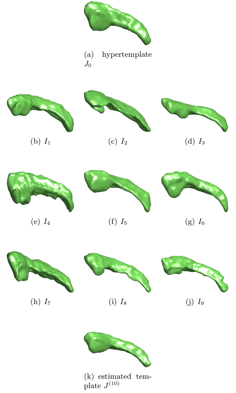
Shown in Figure 2 is an example of template estimation of 3D hippocampus data. Panel (a) is the hypertemplate and panel (b)-(i) are observations. Panel (j) is the estimated template with λ = 0.01.

Figure 2.

Estimating the template from 3D hippocampus data. Panel (a) is the hypertemplate. Panel (b)–(j) are observations I_n, n = 1, 2, …, 9. Panel (k) is the estimated template after 10 iterations. Data courtesy of Biomedical Informatics Research Network.

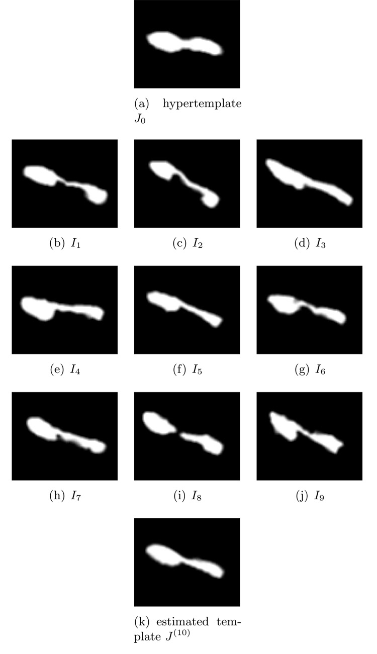
We present sections of the 3D data in Figure 3 to show more clearly that the estimated template adapts to the shapes of observations.

Figure 3.

Section view of 3D hippocampus data. Panel (a) is the hypertemplate. Panel (b)–(j) are observations I_n, n = 1, 2, …, 9. Panel (k) is the estimated template after 10 iterations. Data courtesy of Biomedical Informatics Research Network.

We define the deformation metric, ρ_ℐ(J, I_n) to be square root of the deformation energy, ${\displaystyle {\int }_0^1{\Vert \widehat{\upsilon }\Vert }_V^2}$, for the optimal velocity provided by the LDDMM algorithm. To show that the estimated template is a considerable improvement upon the hypertemplate, we list the metrics ρ_ℐ(J₀, I_n) and ρ_ℐ(J⁽¹⁰⁾, I_n) in Table 1, which are computed with the same parameters. This shows a significant metric reduction from the original hypertemplate to the template estimated after 10 steps.

Table 1.

The metric between observations and J₀, J⁽¹⁰⁾

ρℐ(·, ·)	J0	J(10)
I1	5.2995	4.2773
I2	7.6836	4.1446
I3	4.7706	3.7492
I4	4.9767	2.4993
I5	4.3480	3.3836
I6	4.2751	2.6810
I7	5.3083	3.2349
I8	5.1540	3.4601
I9	5.8151	3.6120

To assess the convergence of the results, we investigate the differences between the estimated templates in successive iterations

$${\Vert J^{\left(k\right)}-J^{\left(k+1\right)}\Vert }_2^2=\frac{1}{S}{\displaystyle \sum _{s=1}^S(J^{\left(k\right)}\left(x_s\right)-J^{\left(k+1\right)}\left(x_s\right)}{)}^2$$ (46)

where S is the number of voxels and k = 0, 1, …, 9. The results are shown in Table 2. We see that the differences between J^(k+1) and J^(k) decrease rapidly to a small value (approximately 0) in the first 10 iterations. This indicates the results converge to a stable shape. In Table 2, we also show the estimated noise levels, which converge too.

Table 2.

Differences between the estimated templates in successive iterations and estimated noise variances.

iteration k	${\Vert J^{\left(k+1\right)}-J^{\left(k\right)}\Vert }_2^2$	σ(k)
0	29.7629	1.0000
1	228.3461	8.5799
2	232.6406	22.1642
3	13.7406	27.1063
4	0.3902	24.5795
5	0.1638	23.8118
6	0.0776	23.6478
7	0.0036	23.5560
8	0.0014	23.5726
9	0.0003	23.5772

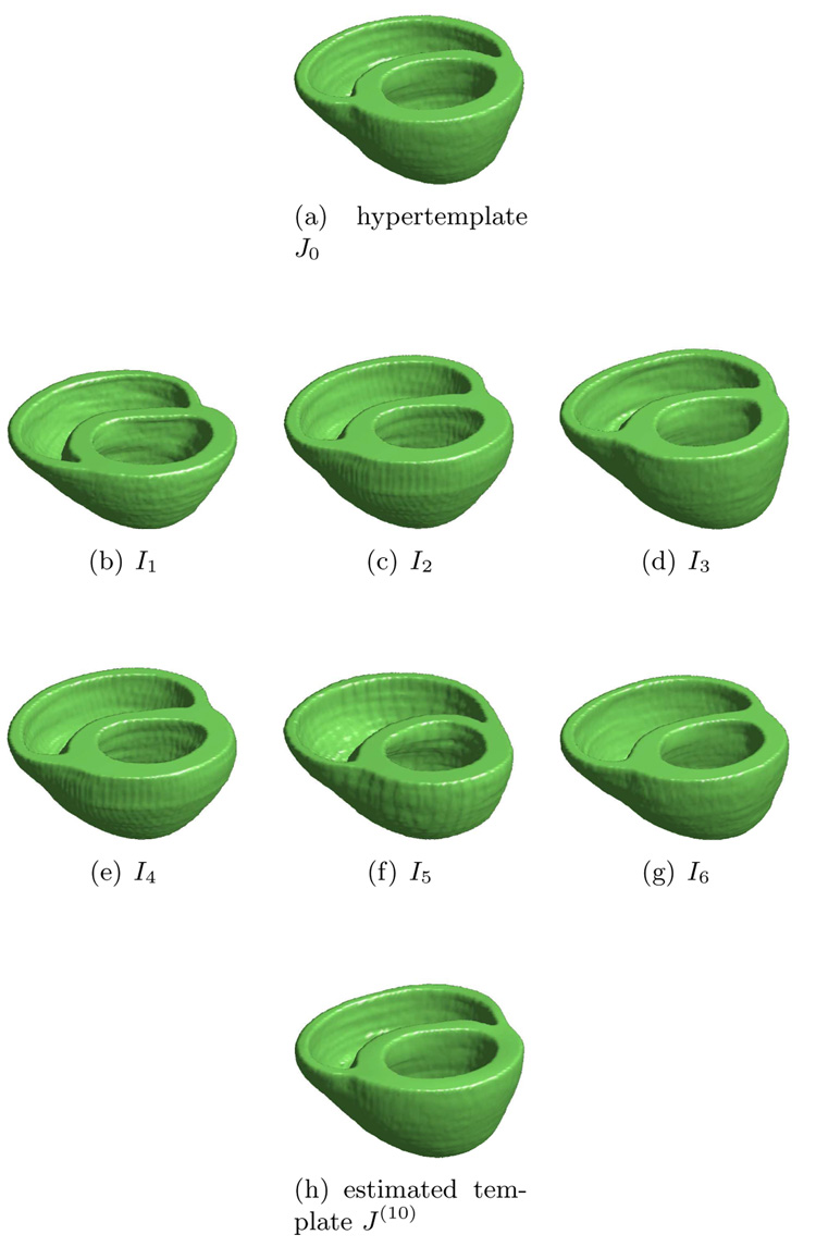
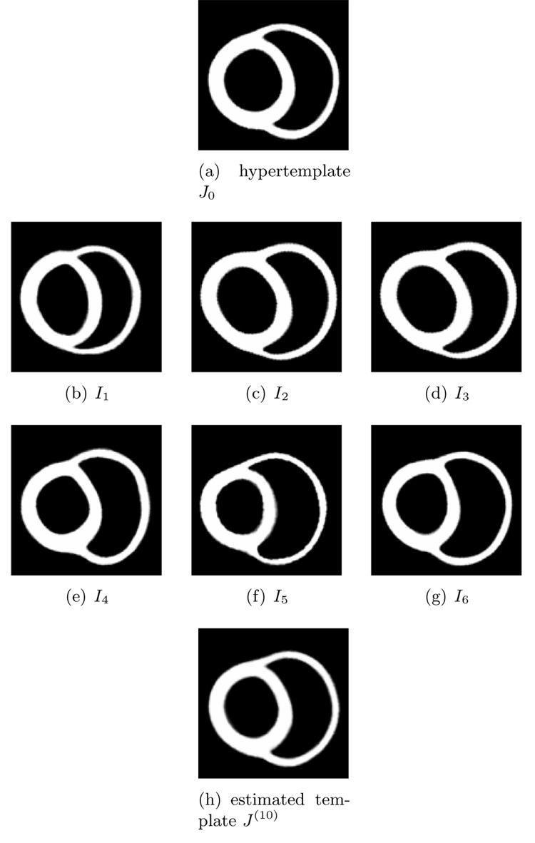
Finally we present the result for 3D heart template estimation. Panel (a) of Figure 4 is the hypertemplate. Panel (b)–(g) are observations I_n, n = 1, 2, …, 6. Panel (h) is the estimated template with λ = 0.0001 at 10th iteration. Figure 5 is the section view.

Figure 4.

Estimating the template from 3D heart data. Panel (a) is the hypertemplate. Panel (b)–(g) are observations I_n, n = 1, 2, …, 6. Panel (h) is the estimated template after 10 iterations. Data courtesy of Dr. Patrick Helm, previously of Dept. of Biomedical Engineering, Johns Hopkins University.

Figure 5.

Section view of 3D heart data. Panel (a) is the hypertemplate. Panel (b)–(g) are observations I_n, n = 1, 2, …, 6. Panel (h) is the estimated template after 10 iterations. Data courtesy of Dr. Patrick Helm, previously of Dept. of Biomedical Engineering, Johns Hopkins University.

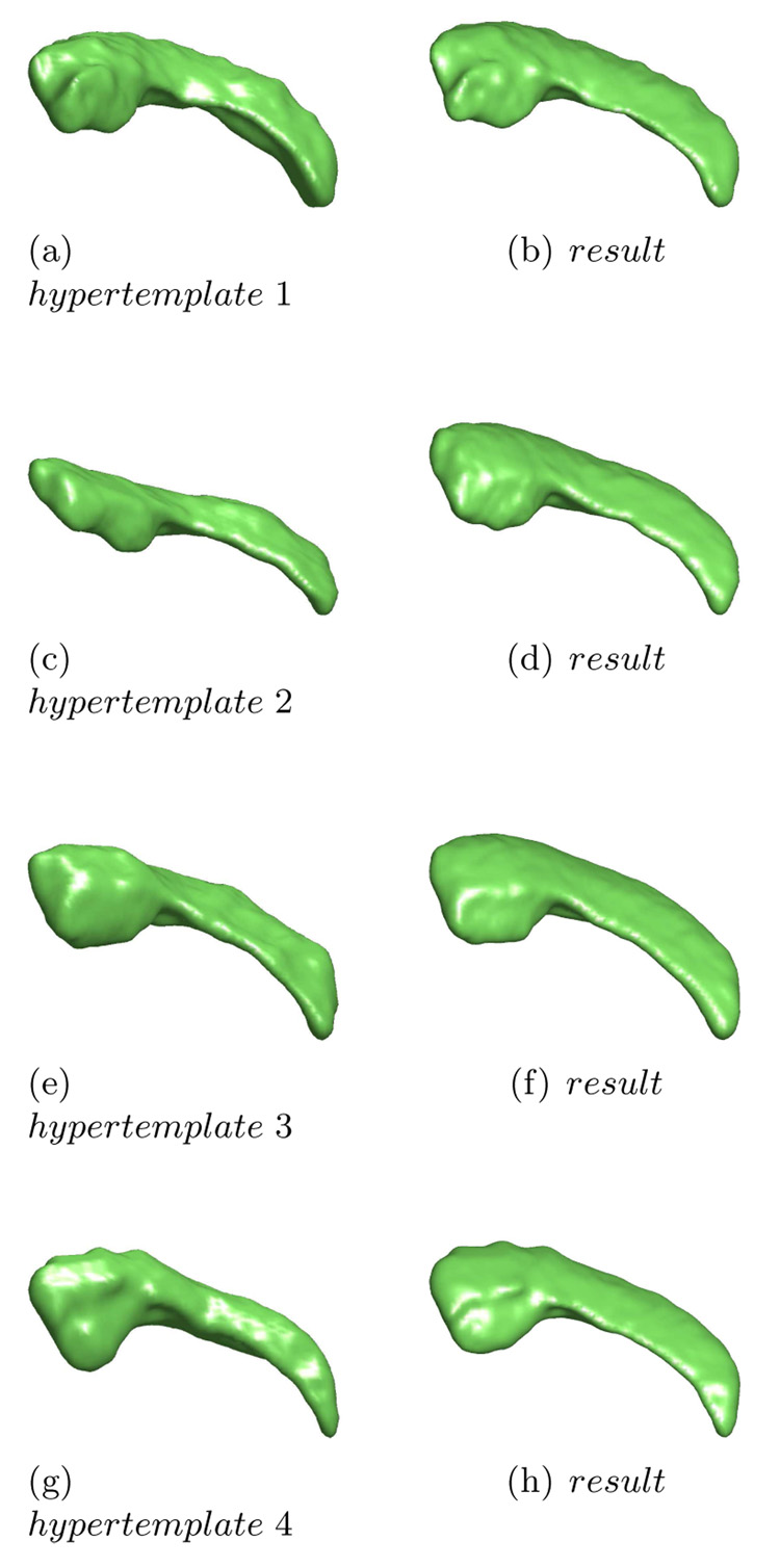
In our model, the hypertemplate is considered as an ”ideal” continuous image with fine structure, which can be provided by an atlas obtained from other studies, although we here simply choose a representative image in the population. Actually, as Figure 6 shows, different hypertemplates yield close results, although they have minor difference.

Figure 6.

For the same observed population, we choose different images as hypertemplate, λ = 0.01. The results only have minor differences.

λ controls how strongly the estimated template depends on the hypertemplate. This has been fixed by hands, but our experiments show a large range of variation without noticeable difference in the final result. By taking small values of λ, the prior reduces to an almost uniform distribution over the orbit of the hypertemplate. We indeed took values between 0.0001 and 1 and obtained stable results.

Remark

In the above model, we assume the initial momenta μ follows a prior distribution p_π(μ) and estimate the template given observations. We call this the “full model”. We can simplify this model by neglecting the prior and just estimate the maximum likelihood of the template J. The MAEM algorithm on this setting will lead us to iterate the procedure of

$${\mathit{Ī}}^{\left(k+1\right)}\left(y\right)=\frac{{\displaystyle {\sum }_{n=1}^N{I}_n\circ g_{{\theta }_n^{\left(k\right)}}\left(y\right)|d_y{g}_{{\theta }_n^{\left(k\right)}}|}}{{\displaystyle {\sum }_{n=1}^N|d_y{g}_{{\theta }_n^{\left(k\right)}}|}}.$$ (47)

The resulting algorithm is similar to [15]. The difference is that the model in [15] warps the observations to match the template and places the white noise between the deformed target and the template, which does not induce a jacobian in the averaging process. However, for a generative model, the logical progression is from template to target. From this point of view, [15] implies an observation noise that is proportional to the inverse jacobian of the deformation, which is hard to justify.

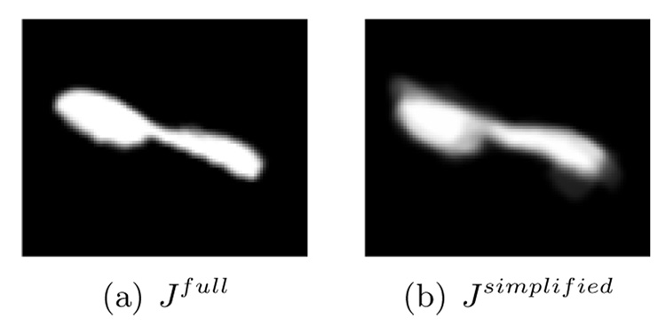
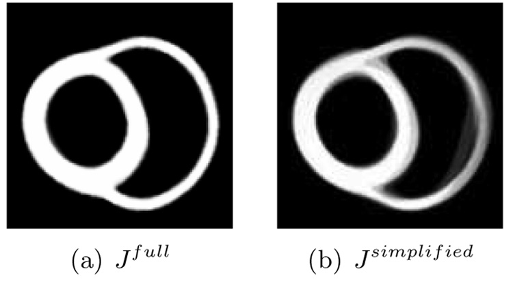
Figure 7 and Figure 8 compare the full model and the simplified model. The simplified model performed relatively poorly compared with the full model that used the prior. This discrepancy comes from the fact that we simultaneously estimate the template and the noise variance. This estimated value of the noise variance allows for some difference between the deformed template and the targets, yielding fuzzy boundaries in the simplified model. If we set the noise variance to a small number, we may obtain sharper boundaries using the simplified model, but this would estimate a template essentially as a metric average (a Fréchet mean) of the targets and would not be consistent with our generative model.

Figure 7.

The template estimation results of full model and simplified model for hippocampus data. Data courtesy of Biomedical Informatics Research Network.

Figure 8.

The template estimation results of full model and simplified model for cardiac data. Data courtesy of Dr. Patrick Helm, previously of Dept. of Biomedical Engineering, Johns Hopkins University.

5 Conclusion

In conclusion, we have presented in this paper a Bayesian model for template estimation in CA. By the momentum conservation law, the space of initial momenta is a linear space where statistical analysis can be applied. It is assumed that observed images I₁, I₂, …, I_N are generated by shooting the template J₀ through gaussian-distributed random initial momenta θ₁, θ₂, …, θ_N. The template J is modeled as a deformation from a given hypertemplate J₀ with initial momentum μ, which has a gaussian prior. This allows us to apply an generalized EM algorithm MAEM to computing the Bayesian estimation of the initial momentum μ, where the conditional expectation of the EM is approached by a Dirac measure, so that one can take the advantage of the LDDMM algorithm. The MAEM procedure finally leads to an image mapping problem from J₀ to Ī with Jacobian weight α in the energy term, which is solved by the weighted Euler-Lagrange Equation. In particular, we apply this method to template estimation for hippocampus and cardiac images. We show that the estimated template is “closer” to observations compared to the hypertemplate, and the differences between the estimated templates in successive iterations decrease to almost 0, which indicates the convergence of the algorithm. We also show the results are stable with different hypertemplates.

References

- 1.Allassonnière S, Amit Y, Trouvé A. Toward a coherent statistical framework for dense deformable template estimation. Journal of the Royal Statistical Society Series B. 2007;69(1):3–29. [Google Scholar]
- 2.Arnold VI. Sur un principe variationnel pour les ecoulements stationnaires des liquides parfaits et ses applications aux problèmes de stabilité non linéaires. Journal de Mécanique. 1966;5:29–43. [Google Scholar]
- 3.Arnold VI. Mathematical Methods of Classical Mechanics. Second Edition: 1989. Springer; 1978. [Google Scholar]
- 4.Avants BB, Gee JC. Geodesic estimation for large deformation anatomical shape averaging and interpolation. NeuroImage. 2004;23 supplement 1:S139–S150. doi: 10.1016/j.neuroimage.2004.07.010. [DOI] [PubMed] [Google Scholar]
- 5.Avants BB, Gee JC. Symmetric geodesic shape averaging and shape interpolation. ECCV Workshops CVAMIA and MMBIA. 2004:99–110. doi: 10.1016/j.neuroimage.2004.07.010. [DOI] [PubMed] [Google Scholar]
- 6.Beg MF, Khan A. Computation of average atlas using lddmm and geodesic shooting; IEEE International Symposium on Biomedical Imaging; 2006. [Google Scholar]
- 7.Beg MF, Miller MI, Trouvé A, Younes L. Computing large deformation metric mappings via geodesic flows of diffeomorphisms. International Journal of Computer Vision. 2005;61(2):139–157. [Google Scholar]
- 8.Dupuis P, Grenander U, Miller MI. Variational problems on flows of diffeomorphisms for image matching. Quarterly of Applied Mathematics. 1998;56:587–600. [Google Scholar]
- 9.Fletcher PT, Joshi S, Lu C, Pizer SM. Principal geodesic analysis for the study of nonlinear statistics of shape. IEEE Transactions on Medical Imaging. 2004;23(8):995–1005. doi: 10.1109/TMI.2004.831793. [DOI] [PubMed] [Google Scholar]
- 10.Glasbey CA, Mardia KV. A penalized likelihood approach to image warping. Journal of the Royal Statistical Society. 2001;63(3):465–492. [Google Scholar]
- 11.Grenander U. General Pattern Theory. Oxford Univ. Press; 1994. [Google Scholar]
- 12.Guimond A, Meunier J, Thirion JP. Average brain models: A convergence study. Computer Vision and Image Understanding. 2000;77(2):192–210. [Google Scholar]
- 13.Helm PA, Younes L, Beg MF, Ennis DB, Leclercq C, Faris OP, McVeigh E, Kass D, Miller MI, Winslow RL. Evidence of structural remodeling in the dyssynchronous failing heart. Circulation Research. 2006;98:125–132. doi: 10.1161/01.RES.0000199396.30688.eb. [DOI] [PubMed] [Google Scholar]
- 14.Holm DD, Marsden JE, Ratiu TS. The Euler–Poincaré equations and semidirect products with applications to continuum theories. Advances in Mathematics. 1998;137:1–81. [Google Scholar]
- 15.Joshi S, Davis B, Jomier M, Gerig G. Unbiased diffeomorphic atlas construction for computational anatomy. NeuroImage; Supplement issue on Mathematics in Brain Imaging. 2004;23 Supplement 1:S151–S160. doi: 10.1016/j.neuroimage.2004.07.068. [DOI] [PubMed] [Google Scholar]
- 16.Le H, Kume A. The Fréchet mean shape and the shape of means. Advances in Applied Probability. 2000;32:101–113. [Google Scholar]
- 17.Marsden JE, Ratiu TS. Introduction to Mechanics and Symmetry. Springer; 1999. [Google Scholar]
- 18.Miller MI, Trouvé A, Younes L. On the metrics, Euler equations and normal geodesic image motions of computational anatomy; Proceedings of the 2003 International Conference on Image Porcessing, IEEE; 2003. pp. 635–638. [Google Scholar]
- 19.Miller MI, Trouvé A, Younes L. Geodesic shooting for computational anatomy. Journal of Mathematical Imaging and Vision. 2006 January;24(2):209–222. doi: 10.1007/s10851-005-3624-0. [DOI] [PMC free article] [PubMed] [Google Scholar]
- 20.Mio W, Srivastava A, Joshi S. On shape of plane elastic curves. International Journal of Computer Vision. 2007;73(3):307–324. [Google Scholar]
- 21.Pennec X. Intrinsic statistics on riemannian manifolds: Basic tools for geometric measurements. Journal of Mathematical Imaging and Vision. 2006;25(1):127–154. [Google Scholar]
- 22.Trouvé A. An infinite dimensional group apporach for physics based model. technical report. 1995 (electronically available at http://www.cis.jhu.edu). unpublished.
- 23.Vailliant M, Miller MI, Younes L, Trouvé A. Statistics on diffeomorphisms via tangent space representations. NeuroImage. 2004;23:S161–S169. doi: 10.1016/j.neuroimage.2004.07.023. [DOI] [PubMed] [Google Scholar]