Biochemical Individuality Reflected in Chromatographic, Electrophoretic and Mass-Spectrometric Profiles

Abstract

This review discusses the current trends in molecular profiling for the emerging systems biology applications. Historically, the methodological developments in separation science were coincident with the availability of new ionization techniques in mass spectrometry. Coupling miniaturized separation techniques with technologically-advanced MS instrumentation and the modern data processing capabilities are at the heart of current platforms for proteomics, glycomics and metabolomics. These are being featured here by the examples from quantitative proteomics, glycan mapping and metabolomic profiling of physiological fluids.

1. INTRODUCTION

The rapidly developing fields of genomics, proteomics, glycomics, and metabolomics have largely been driven by the methodological/technological advances in biomolecular mass spectrometry and microscale separation science. Additionally, greatly improved computational capabilities to deal with complex information (bioinformatics) have become readily available When extensive and detailed analytical data are increasingly reported in the open literature, particularly in many new and technique-specialized journals, without explanations of their biochemical meanings or even trends, the time becomes appropriate for some generalization, reflections, and feedback on the direct and indirect causes and attributes of the “omics revolution.” Our specialized fields are finding their integration in the area of the newly promoted “systems biology” [1–4].

This brief review article deals with the subject of “biochemical individuality” from the point of view of our methodological constraints and discusses the current views and their historical connections to some earlier studies in metabolic profiling. This term generally implies that a living system under normal or standard conditions is broadly characterized by its unique set of biochemical parameters, particular compounds and substrates, enzymatically catalyzed reactions, etc., which may or may not be easily measurable by molecular profiling techniques at hand. As is known that simple microorganisms, and even their more or less virulent strains, differ in biological activity and interactions with their host, the differences in their biochemical individuality (molecular makeup) are automatically assumed. In multicellular, and thus more morphologically and biochemically complex systems, we measure or profile a certain integrated output, which is a function of altered biochemical individuality of, for example, a diseased individual in comparison to normal. This is not to say that normal organisms may not differ amongst themselves, however slightly, in their metabolic rates and biomolecular composition under somewhat different conditions of physical exercise and diet, and to a larger degree, in their gender and genetic makeup. While our desire to utilize molecular profiling for the benefits of biomedical research, improvements in human conditions, and the design of more effective pharmaceuticals in the future is likely to remain the centerpiece of this field, there are additional implications for developmental biology, neurobiology, nutrition, plant sciences, chemical ecology, etc.

The current understanding of biological processes at the molecular level has been greatly facilitated by the advances in bioanalytical chemistry over the past two decades. We briefly discuss the evolution of different measurement concepts and data interpretation tools. As three examples of the fields in which some progress has been made, we feature first quantitative proteomics and its role in disease biomarker discovery, followed by the recent uses of quantitative, high-sensitivity glycomics in cancer research and, potentially, diagnosis and prognosis. Finally, as an evident area of connecting genes with small metabolites, we discuss some recent research on chemosignaling in Nature.

2. FROM METABOLIC PROFILING TO SYSTEMS BIOLOGY

Every living organism in its environment represents a biochemically unique system whose vital functions can be probed through analytical measurements. Beyond the morphological recognition of different types of cells, which has been the basis of biological observations for a long time, we are now routinely capable of making a number of isolated analytical measurements which may help us in assessing the state of health or “normalcy” within the organisms under study. While this is true as much for small biological entities, i.e., microorganisms or primitive plants, as it is for the more advanced eukaryotic systems, the multicellular organism represents more challenging conditions and opportunities for our bioanalytical measurements. Yet, these methodologically unrelated and relatively simple analytical measurements can still be correlated to yield a biologically useful picture. This is easily exemplified in any case when a physician requests a battery of clinical tests to be performed on a patient’s blood sample. In such undertaking, he/she is being assisted by the knowledge of clinical chemistry and epidemiology that has often been in practice for many years. Not only does an experienced clinician learn about this patient’s primary condition, such as possibly a diabetic condition or one of the inborn errors of metabolism, but additional health-related information may also exist due to the remainder of clinical measurements. Unusual results from a clinical laboratory often lead to additional and more sophisticated clinical tests, frequently those based on antibody-determined “biomarkers” of a disease. While considerable progress has been made over the years in clinical diagnosis through biochemical measurements, an intensive search for additional disease biomarkers is still as alive as ever.

In general terms, biomarkers are indicators of a biological process or perturbation in a complex system as a result of a disease or its progression. These could be genes, proteins or unique posttranslational modifications of proteins, or small biological molecules and other products of metabolic pathways. Appropriate biomarkers are expected to provide valuable information for selection of a medical treatment or prediction and measures of outcome. In the current situation with biomarker discovery procedures, investigators using different molecular profiling technologies usually look at a vast number of biological sample components such as gene expression arrays (genomics and transcriptomics), complete peptide maps from digested protein mixtures (shotgun proteomics), deglycosylation products from glycoprotein mixtures (glycomics), or complex profiles of endogenous metabolites (metabolomics). Since a number of individuals and their profiles have to be judged on a statistical basis, search for putative biomarkers amounts to looking for a needle in a haystack without the use of reliable computer-aided techniques for pattern recognition. This connection between the advanced profiling methodologies and the data analysis has been occasionally found successful in preliminary indentification of putative biomarkers, as will be shown below with and example of the principal component analysis (PCA) of glycomic profiling data in cancer diagnosis. The so-called PCA loading plots can subsequently aid in the identification (structural elucidation) of components responsible for distinction. The ultimate goal is to identify a biomarker or a set of biomarkers with the greatest possibility for the risk assessment (preventive medicine), early diagnosis of a disease, and prognosis.

The biocomplexity issues have increasingly been recognized in contemporary science and, more specifically, in the context of the currently popular “systems biology” [1–4]. For several decades, this exciting and technologically-driven area of current human endeavor has had its philosophical basis in the early realization of the value of multicomponent analyses, rather than isolated analytical measurements. While the techniques of Williams [5] and other researchers were rather primitive at the time, he was able to define criteria for the individual variation in human biodiversity and suggested that characteristic metabolite patterns could be obtained from patients suffering from different diseases. After Dalgliesh et al. [6] demonstrated that it was possible to obtain multicomponent gas-chromatographic (GC) analyses of the derivatives for a variety of trace organic compounds present in urine and tissue extracts, Horning and Horning [7,8] introduced the term “metabolic profiles”, defining the patterns of biochemically related metabolites. These approaches hinge philosophically on the concept of “orthomolecular medicine”, promoted at one time by Linus Pauling [9]. As our biochemical knowledge of the physiological processes improves with time, this concept remains as topical as ever.

Clearly, chromatography made significant inroads already decades ago into getting us a bit closer to a complete biochemical knowledge of the living systems. First, the advent of gas-liquid chromatography and its new sensitive ionization detectors developed during the late 1950s and throughout the 1960s set the tone for chromatography as a quantitative analytical method for multicomponent determinations. Subsequent studies by different research groups, leading to conversion of polar biological compounds (steroids, sugars, urinary acids, etc.) into the derivatives amenable to GC analysis, have enormously expanded the scope of biomedical GC applications. A nearly coincident development of capillary GC, and GC-MS in particular, for biochemical separations and measurements has added the necessary resolution, sensitivity and identification power to study a wide range of biologically important molecules. Naturally, the scope of metabolomic investigations became significantly enriched two decades later when the combination of liquid chromatography with mass spectrometry (LC-MS) and other relevant technologies started to facilitate detection and quantitative profiling of the many biological compounds which were outside the reach of GC-MS-based techniques. These developments will be mentioned further in the sections below.

The primary practical aim of quantitatively profiling various body fluid and tissue constituents has been to define the biochemical status in health and disease. It has been summarized appropriately by Jellum [10] many years ago in that “it seems reasonable to assume that if one were able to identify and determine the concentration of all compounds inside the human body, including high molecular weight as well as low molecular weight substances, one would probably find that almost every known disease would result in characteristic changes of the biochemical composition of the cells and the body fluids.” While the separation and biomolecular mass-spectrometric technologies and the bioinformatics tools of today are formidable, they are probably still very far from delivering a full inventory of all constituents of body fluids and tissues.

The biochemical individuality has been recognized as an experimental complication of acquiring data from human subjects and, to a lesser degree, experimental animals. This is a somewhat parallel problem to distinguishing between the “apparently healthy” and “diseased” individuals in clinical chemistry assays where considerable ranges for both often exist. In humans, physical exercise, seasonal and diurnal variations, nutritional status, genetic background and ethnicity, physiological or pathological status have all been recognized as important even in clinical assays based on isolated determinations [11]. In the near future, the variables that cannot be easily controlled must be consequently accounted for in large-scale profiling studies. To what degree the most efficient tools of the “omics revolution” will deal with the obvious biochemical complexity of such biological systems is yet to be seen.

The systems biology provides a "holistic" approach to sorting out a vast body of biochemical information provided by the rapidly developing fields of genomics, transcriptomics, proteomics, glycomics, and metabolomics. Following the Human Genome Project and the following efforts to characterize the genomes of model animals, the overwhelming task of characterizing the corresponding proteomes with their voluminous posttranslational modifications has preoccupied many specialized laboratories. The unprecedented advances in biomolecular characterization and quantification of proteins in physiological fluids and tissues seem to provide foundation for further inquiries into the corresponding glycomes and metabolomes.

A narrow view of the biomarker concept can lead to misinterpretation of the virtues of molecular profiling. Even the commonly measured attributes of diseases, such as glucose levels in diabetes or a number of other disease-related quantitative changes in plasma proteins, are seldom satisfactory to define patients’ conditions. For example, serum prostate-specific antigen (PSA) is used clinically to screen for prostate carcinoma [12]. A PSA level greater than 4 ng/mL is considered to be indicative of potential prostate cancer; however, the specificity of this test is far from being satisfactory [13]. There is only 25% likelihood of having prostate cancer, if the PSA values are between 4 and 10 ng/mL. Prostate cancer may be present even when the PSA concentration is below 4 ng/mL, while it may be absent even at elevated PSA concentration which has been attributed to non-cancerous prostate diseases[13]. It is becoming increasingly appreciated that multiple biomarkers should be investigated, and that the early molecular markers of a disease may be different from those in its advanced stages. A significant virtue of the systems biology will undoubtedly be a mutual biochemical inclusiveness of different molecular profiling techniques together with the possibilities of dynamic modeling[14,15].

The dynamic aspects of a biomarker behavior are shown in Figure 1, according to van der Greef et al. [4], illustrating its temporal fluctuations in homeostasis and progression into different stages of a disease. Finding important biomarkers at the early stage of diseases is obviously a very important goal of biomedical research, which will require a scientific “synthesis” of many molecular profiling experiments involving human samples as well as appropriate animal models.

Figure 1.

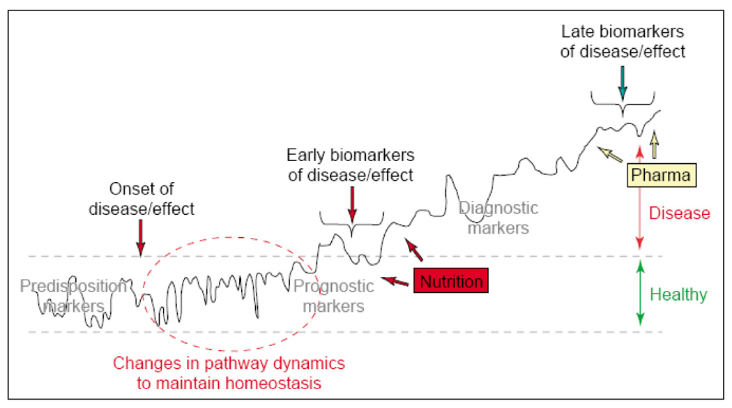
The development of disease from healthy (homeostasis within black-dotted lines) to sub-optimal health and eventually an overt disease state. Biomarker patterns (for graphical reasons represented as a single line) are essential to describe the changes from normality to dysfunction. Reproduced from [4] with permission.

3. EVOLUTION OF MOLECULAR PROFILING TECHNIQUES

Throughout the history of chromatography and electrophoresis development, we are often reminded that the capability of quantifying and analytical throughput are the essential ingredients of success in applying a particular technique to a significant biomedical problem. While the ideas of most pioneers of metabolic profiling were basically sound, they had to struggle, in their times, with rather primitive technologies to acquire seemingly complex biochemical data. From all chromatographic methodologies, gas chromatography (GC) was the first to obtain the multicomponent analyses of urine and tissue extracts, including aliphatic and aromatic acids, polyols, steroids, as well as their glycine and glucuronide conjugates [6]. With most biochemicals being thermally labile, this was only possible after the development of sample chemical derivatization techniques which stabilize such solutes.

It has become increasingly clear from today’s perspective that molecular profiling studies can only be successful if they readily provide at least the following attributes: (a) adequate resolution of most, if not all, important mixture components; (b) unequivocal structural identification/verification of the components to be measured and quantified; and (c) reliable quantification with the necessary measurement precision, so that the measurement errors do not exceed the genuine differences due to the individual profiles distinguishing different study subjects. Most biochemical applications of GC throughout the 1970s reflect these goals: development of capillary GC for biochemical measurements [16–21]; a coincidental availability of its combination with mass spectrometry (GC-MS) for important metabolite identifications; and, the overall improvements in the reliability of capillary GC as a sample profiling technique in terms of sampling and instrumentation [21]. Most of these issues appear paralleled in a later development of metabolomic approaches based on NMR spectrometry [22,23], an inherently quantitative technique, which also provides structural identification, yet on the basis of different physical principles. In certain applications, the NMR-based techniques feature distinct advantages of a minimum sample preparation and techniques’ non-destructive nature. On the other hand, they are often bound to miss minor, yet biologically important, components due to the general lack of sensitivity. Regardless, the earlier studies on the metabolic profiling concepts met with only a modest response from the biomedical community and, ironically, the subject is now being revisited with the introduction of Human Metabolome Database and a discussion of its comparative merits with the results of genomic and proteomic initiatives [24].

One additional, very important attribute of molecular profiling is comprehensiveness. With their inherent constraints of solute volatility, capillary GC and GC-MS could hardly cover a wide range of polar metabolites and other biomolecules. The attempts for sample derivatization (see reference [25] for a review) or degradation of biomolecules through pyrolysis [26] brought only a marginal progress concerning this problem. While the advent of high-performance liquid chromatography (HPLC) removed the limitations of molecular migration for non-volatile and large molecules, the inherent problems of detection and solute identification have hindered progress in the area. The earlier attempts for screening biological fluids by HPLC met with a limited success, when the detection techniques were largely favoring UV-absorbing, fluorescent, or electrochemically active solutes, without the availability of LC-MS for structural identification.

Among the early GC- and GC/MS-based applications to metabolic profiling, the separation of volatile body fluid components without derivatization [19,27] has gained particular importance to research in our laboratory aiming at the recognition of molecular attributes of diabetes and oxidative stress [28–32] as well as in the identification of selective messengers of physiological state and identity (pheromones) [33–35]. As an illustration of the state-of-the-art in this area during the 1970s, we show the separation of human volatile urinary profiles (Figure 2) and their minor variations with diet on three consecutive days of 24-hr urine collections [19] for a single individual. Similar techniques were also developed for other physiological fluids. With the high resolution of capillary GC columns, the availability of GC-MS for identification, and the early applications of chemometrics to these complex profiles [28,29], this part of the field was ready for meaningful biomedical applications well before the genomic era. While the earlier sample enrichment techniques in this area were recently replaced by the more quantitative and versatile methods based on fiber microextraction [36] and the stir bar sorptive approach [37,38], this area still hold significance to the current efforts in modern metabolomics.

Figure 2.

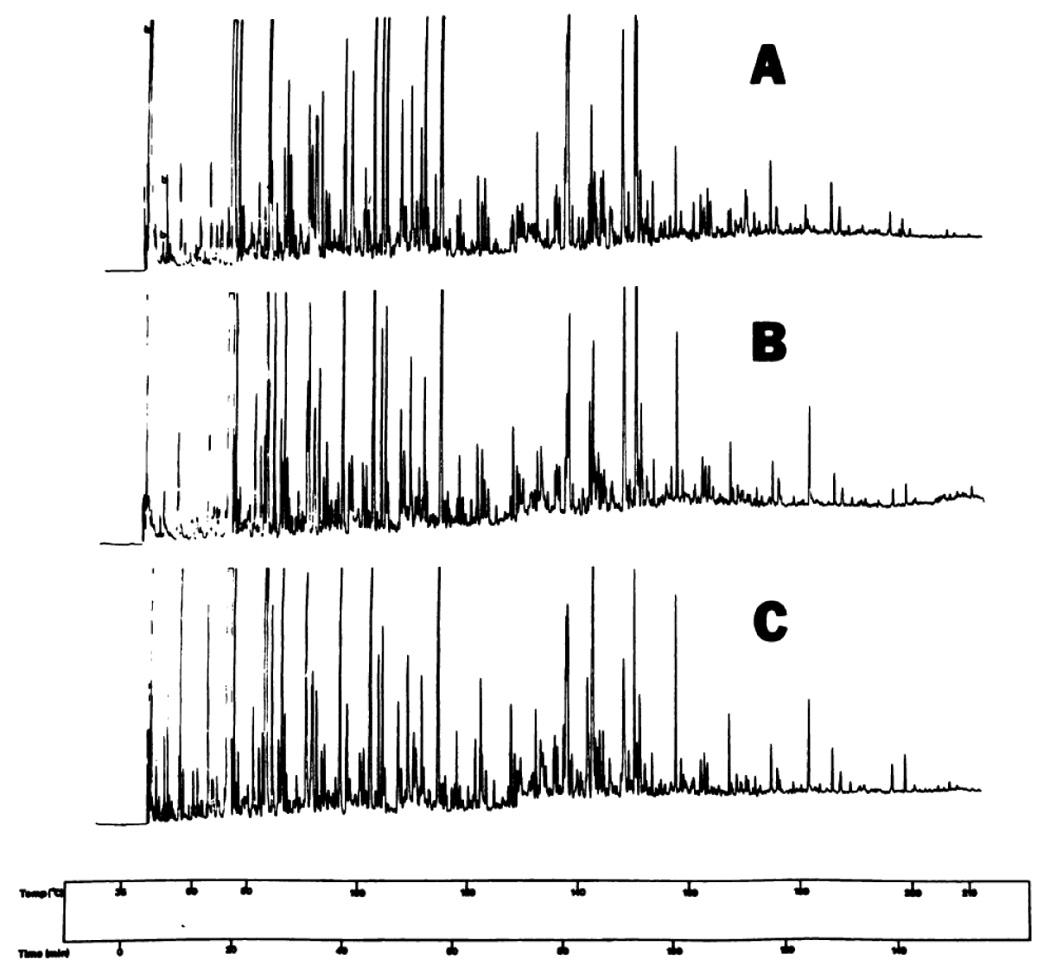
Chromatograms of urinary volatiles of a normal man. A and B are from 24-h, urines collected on different days and analyzed successively. B and C represent aliquots of the same urine, analyzed on different days. Peaks owing to the precolumn blank are designated as b in chromatogram A (left). Chromatographic conditions: 80 m × 0.31 mm (i.d.) glass capillary column coated with SF-96 silicone oil. Temp. (°C) time (min) are shown in all figures at top and bottom, respectively. Reproduced from [19] with permission.

Metabolic profiling through GC-MS of derivatized polar compounds, such as steroids [18,39] and urinary acids [40] were less commonly pursued by clinical and biomedical research laboratories, presumably due to their procedural complications and the difficulties of interpreting mass spectra of derivatized compounds.

Without any doubt, the introduction of electrospray ionization (ESI) and matrix-assisted laser desorption-ionization (MALDI) to mass spectrometry (MS) during the late 1980s has revolutionized the field of biomolecular analysis. It has made it feasible to analyze intact proteins, peptides, nucleotides, glycoconjugates, and other biomolecules, giving thus rise to the new fields of proteomics and glycomics and their new subdisciplines termed “glycoproteomics”, “neuropeptidomics”, “lipidomics”, “O-GlcNAc-proteomics”, etc. Both substantial and gradual improvements in virtually all aspects of the MS instrumentation, perhaps most notably in the mass analyzer area and detector technologies, have now been the major driving force for continuation of the “omics revolution”. Together with the enormous capabilities of today’s data acquisition, processing and interpretation (bioinformatics), the contemporary mass spectrometry, especially its tandem (MS/MS) instruments, are increasingly finding their match in the high-performance (capillary) separation techniques which effectively fractionate and separate the myriads of biological molecules.

Whenever a separation of complex biological mixtures is required, capillary separation techniques are almost invariably employed in virtually all contemporary investigations of the systems biology. Capillary separations in the condensed phase have their historical link to the developments of miniaturized separation systems in chromatography [41–45] and electrophoresis [46] in the late 1970s and the early 1980s, followed by the more recent introduction of microfabricated separatory channels [47,48] and the so-called “lab-on-the-chip” analytical approach. While liquid chromatography (LC) packed capillary columns of today’s proteomic and metabolomic procedures have mostly been based on the small-diameter type developed by Karlsson and Novotny [49] and Kennedy and Jorgenson [50], some current trends also emphasize the use of monolithic columns (for a review, see reference [51]) and ever smaller particle size, currently at 1–2 µm [52,53]. In the jargon of today’s proteomics or metabolomics, it is becoming more common to hear about “microflow” (above 1 µL/min) and “nanoflow” (below 1 µL/min) systems, rather than column types themselves, presumably due to their connection to MS.

Besides the efficiency advantages of capillary LC and electrophoresis, there are biochemically important attributes of the miniaturized separation systems [54], such as their compatibility with MS, increased mass sensitivity of concentration-sensitive detectors, better inertness toward sensitive biomolecules, such as proteins during microisolation, compatibility with small samples and small biological objects, such as laser dissection preparations and single biological cells [54]. As an example of the state-of-the-art biochemically important application from the 1980s, we demonstrate in Figure 3 a chromatogram of solvolyzed plasma steroids on a packed capillary column [55]. The hydroxysteroids were fluorescently labeled to ensure their detection through the laser-induced fluorescence. Such separations at that time suffered from relatively long analysis times, as contrasted by the more recent proteomic application (Figure 4) where considerably greater resolution of peptides is demonstrated at shorter analysis times [56] using a capillary of a smaller diameter and much smaller particle size. The advantages of small-particle columns, operating under very high inlet pressures, were also recently shown in metabolomic studies [57,58].

Figure 3.

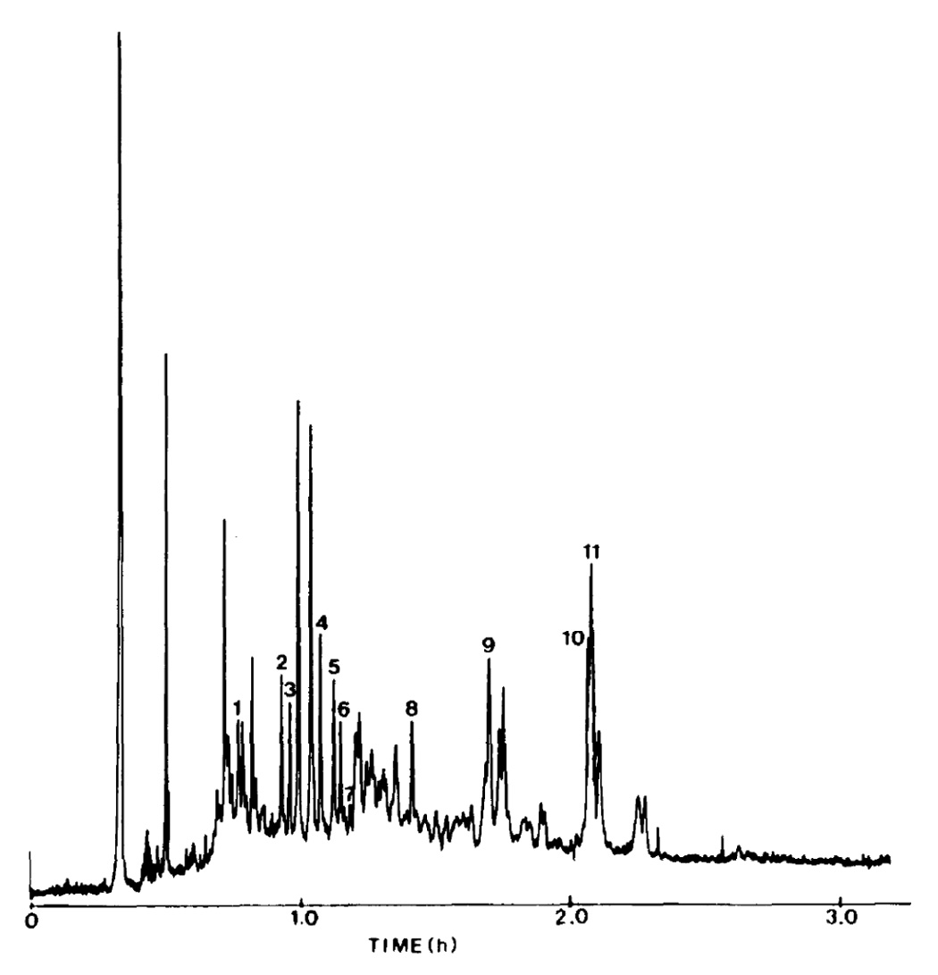
Chromatogram of solvolyzed plasma steroids. Chromatographic conditions: column, 2.25 m × 220 pm I.D. packed with 5-µm Spherisorb ODS; mobile phase: continuous gradient 75–100% aqueous acetonitrile (1.5 µl/min); injection, approximately 50 pg of each steroid was injected. Tentatively identified components: 1 = 5α-androstan-3α,11β-diol-17-one; 2 = 5β- androstan-3α,11β-diol-17-one; 3 = 5β-pregnane-3α, 11β,l7α,21-tetrol-20- one; 4 = 5β-pregnane-3α,17α,20β,21-tetrol-11-one; 5 = 5β-pregnane-3α,- 11β,17α-20α,21-pentol; 6 = 5β-pregnane-3α,17α,20α,2l-tetrol-11-one; 7 = 5β- pregnane-3α,11β,17α,20α,-21-pentol; 8 = 5α-androstan-3α-ol-17-one; 9 = 5- androstene-3β-ol-17-one; 10 = 5β-pregnane-3α,20α,21-triol; 11 = 5β- androstan-3α,17β-diol. Reproduced from [55] with permission.

Figure 4.

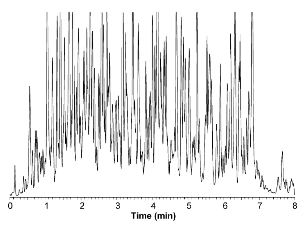
RPLC-MS base peak chromatogram the S. oneidensis global tryptic digest sample. Conditions: the 5-µL sample loop was used to load 1 µg of the sample onto a 20 cm × 50 µm i.d. packed capillary for LC separation. MS with an m/z range of 400–2000 was used for detection. Reproduced from [56] with permission and modification.

4. ANIMAL MODEL SYSTEMS

Precision and accuracy of analytical measurements have special meaning in the multicomponent investigations of any biological material. Whether we acquire protein profiles or closely related metabolite chromatograms of two genetically diverse microorganisms under different culture conditions for the sake of comparison, or analyze different patients’ blood sera through the same type of analytical instruments, the sample preparation and the use of internal standards may differ substantially. Just as with the routine measurements carried out daily in clinical laboratories, the serial measurements of molecular profiles greatly benefit from procedural automation and careful optimization of a multistep sample treatment. This is evident today with the efforts of developing analytical platforms for proteomic and glycomic measurements through the maximum use of liquid dispensers, automated sampling valve systems, commercial 96-well plates, etc.

In molecular profiling studies of human samples, the inherent biochemical variations within a population necessitate careful statistical comparisons of results, leading naturally to a wide use of multivariate statistical methods. In parallel, the large sets of clinical samples necessitate greater analytical throughput. The recent success in identifying some disease biomarkers notwithstanding, the current proteomic investigations (based on different combinations of the separation techniques and mass spectrometry) tend to be tedious and slow due to the inherent complexity of proteomes. The multimethodological nature of proteomic, glycoproteomic and glycomic investigations often tends to resort to the use of isotopic labeling in comparative quantitative studies. It is often the inherent advantage of the MS-based detection that the isotopic labeling can be widely utilized.

The biochemical variability of humans is a less complicating influence in the studies where a subject in different stages of a disease or in the course of disease treatment serves as “its own control” in molecular profiling studies. For example, a patient’s blood sample is drawn at the time of disease diagnosis, repeatedly during a treatment time and, finally, in remission. Comparative profiling analyses are subsequently performed to yield potential insights into the biochemical differences between health and disease. Thanks to a number of insightful clinicians, some sample banks exist around the world with highly valuable samples from the patients before the onset of a disease and after, or additional samples collected from the family members, siblings, identical twins, etc. A remarkable case of the genetic influence emerged during a study in our laboratory profiling 24-hr urine samples of two male identical twins (Figure 5), who were hospitalized and maintained on identical diets for a one-week period. The chromatograms are remarkably similar and quite different from the other individuals included in the overall study [59].

Figure 5.

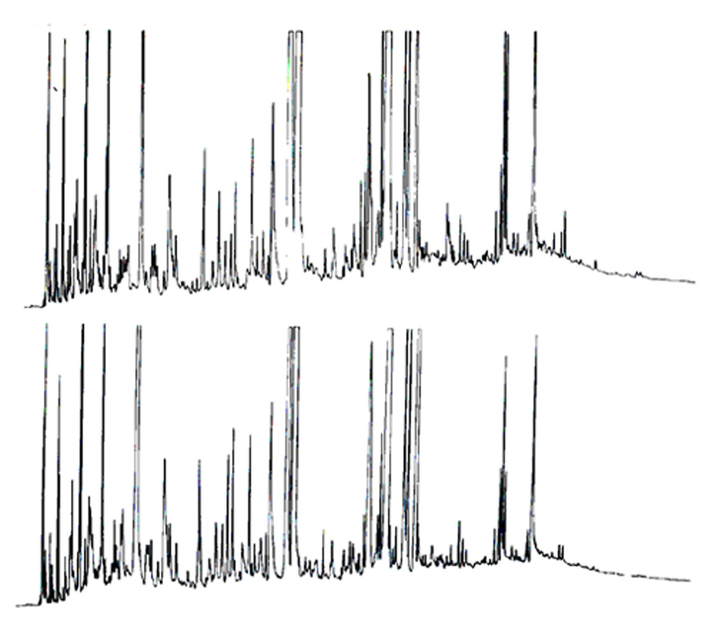
Volatile chromatographic profiles of identical twins maintained on an identical diet. Chromatograms were obtained on an SF-96 glass capillary column. Temperature programmed from 30–210°C at 2°C/min. Reproduced from [59].

Animal models provide an alternative approach for the cases where human studies are limited by the requirements of large sample sets, ethical considerations, rigid clinical control, or other considerations. A very large number of human disease models exist among experimental animals, including genetically inbred syndromes [60], spontaneously occurring diabetes in rodents [61], nude mice for immunological studies [62], knockout and transgenic mice, etc. Through the comparisons with appropriate control animals, molecular profiling techniques can potentially yield a wealth of information which may not be otherwise easily available.

Through the use of well-defined animal systems, experimental conditions can be adjusted to control diet, environment and exercise. With appropriate ethical safeguards, different metabolic, endocrinological and behavioral manipulations can also be performed that are not feasible with humans (e.g., the use of experimental diets, toxicity testing, selective metabolic blocking agents, or surgical procedures). During tumorigenesis in model rodents, the ability to control the onset, severity and complication of the disease can potentially be utilized to provide unprecedented data through molecular profiling of body fluids and tissue extracts.

The inbred strains of rodents provide a very unique focus on the separation of genetic factors from other potential biological variations. This is perhaps best exemplified by the house mouse strains where such strict genetic control is available that molecular profiling comparisons can be performed between animals differing only in one gene locus, such as with the major histocompatibility genes [63].

5. EXAMPLES OF MOLECULAR PROFILING TECHNIQUES

5.1. QUANTITATIVE PROTEOMIC ANALYSIS AND ITS SUCCESSES AND LIMITATIONS

A search for proteomic biomarkers has recently become both popular and necessary. Additionally, in contrast to the situation with genomes for various organisms, their respective proteomes are relatively dynamic, reflecting their immediate dependence on environmental conditions (system perturbation). Thus, comparing quantitatively the proteomes (with a simultaneously verified protein identity) under different states (e.g., samples originating from different stages of a disease) is an arduous, but necessary task of the field of proteomics. Fortunately, the efficient separation techniques and mass spectrometry, with its high data acquisition capabilities, complement each other in this important task of delivering quantitative information on such complex samples.

Quantitative differences in protein expression can be evaluated by a number of techniques that have evolved either around classical gel electrophoresis or the more modern techniques of LC. While the use of a single migratory dimension in electrophoresis is limited to extensively fractionated proteomes, two-dimensional electrophoresis (2-DE) in polyacrylamide gels remains widely employed in dealing with complex proteomes. Here, different stains are popular for quantitation, while a protease digestion of the isolated protein spots and MS are used for protein identification. The LC-based approaches involve stable-isotope tags, biological incorporation of isotopically-labeled amino acids in cell cultures, or a label-free quantification procedure. Each procedure will be briefly described in the following text, discussing their advantages and limitations.

A. Gel-based Procedures

In the most commonly used procedure, the gels featuring separate samples are run and stained for a side-by-side comparison. While 2-DE gels allow different proteomes to be compared on the basis of their orthogonal migrations according to the isoelectric point and molecular size, respectively, the individual proteins can be visualized through optical density or fluorescence by an appropriate scanner. Next, the spots that appear more intense in one gel over the other are excised for digestion and MS identification. In routine studies, only those spots (proteins) that appear differentially expressed need to be analyzed by MS (Figure 6).

Figure 6.

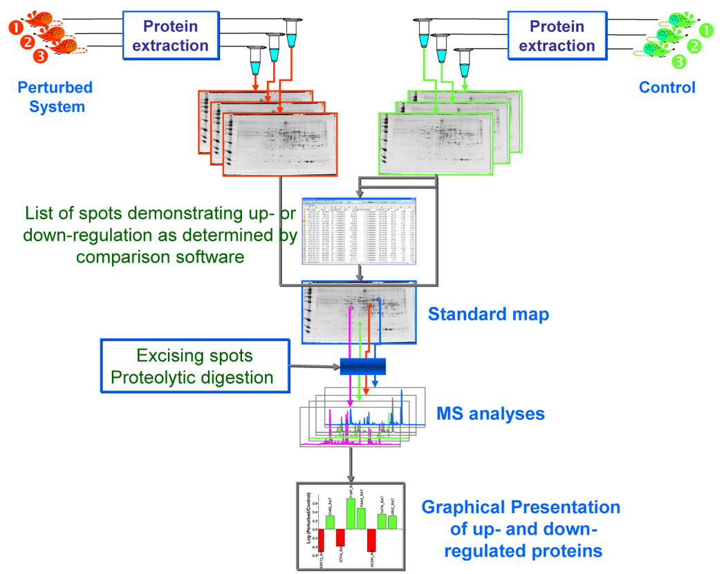
Flow chart depicting the different steps involved in generating sets of 2-D maps derived from control and perturbed biological systems. Proteome samples are extracted from both sets of animals and 2-DE is performed on each sample separately. After gel staining, the two sets of gels are compared using a specialized software such as PDQuest (BioRad, Hercules, CA). This comparison results in the generation of a list of up- and down-regulated spots which are subsequently excised and subjected to proteolytic digestion prior to MS identification. Finally, the identified proteins and their trends as a result of perturbation are graphically represented.

An interesting alternative to the conventional 2-DE systems is differential in-gel electrophoresis, which is based on a differential labeling of the proteome samples with N-hydroxy-succinimide ester-modified cyanine fluorophores that feature different excitation and emission wavelengths. The most popular dyes seem the so-called Cy3 and Cy5, which excite at 540 and 620 nm, and emit at 590 and 680 nm, respectively. Two different proteomes can be separately labeled with either of the two fluorophores, each covalently modifying lysine residues in proteins. Since the two fluorophores have distinct excitation and emission wavelengths, two different proteomic samples can be combined and analyzed in a single 2-DE gel. Specialized 2-DE image analysis softwares can evaluate differences in protein expression (Figure 7).

Figure 7.

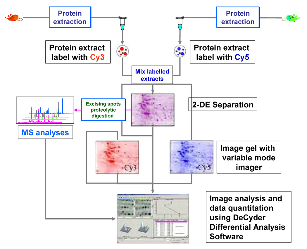
Flow chart depicting the different steps involved in generating of 2-DE using DIGE. Proteome extracted from control and perturbed systems are labeled differentially with the two fluorophores Cys 5 and Cys 3, respectively. The two labeled samples are then mixed and a single 2-DE is performed. The gel is then visualized using two different excitation wavelengths suitable for visualizing both fluorophores. The two images recorded at the different wavelengths are then compared with specific software capable of quantifying based on the intensities observed under the two different conditions employed for measurement. DeCyder Differential Analysis Software is capable of performing such comparison and has been developed by GE Healthcare Bio- Sciences Corp. (Piscataway, NJ).

Gel-based techniques are popular in biological laboratories because of their obvious attraction of visualizing and displaying hundreds of proteins in an easily understandable manner. However, the gel procedures are tedious and time-consuming. They have frequently been criticized for a lack of inclusiveness (e.g., a bias against small and hydrophobic proteins) as well as a lack of reproducibility. However, these criticisms have been to some extent dampened by the development of better reagents, techniques, and gel alignment softwares.

The differential in-gel approach overcomes the gel-to-gel variation problem, offering an improved spot matching, enhancement of sensitivity due to fluorescence, and improvement in dynamic range. However, fluorescent labeling has always its own issues of protein reactivity and contaminants, complicating the following MS analysis and subsequent database searching.

A significant handicap of all gel-based proteomic techniques is their limited dynamic range. With the high sensitivity of today’s mass spectrometers, it is not uncommon to locate significant amounts of proteinaceous material in the blank space between the visualized spots [64]. With serum and plasma as the most commonly used biofluids in biomarker discovery, it is essential to remove the major proteins through a depletion step, in order to be capable of displaying the trace proteins.

B. Chromatographic Procedures

Quantitative proteomics has recently capitalized on major advances in the design and use of chromatographic columns and automated instrumentation. Different platforms may use chromatographic separation, or at least fractionation, at the level of intact proteins prior to their proteolytic digestion and a subsequent separation of the resulting peptides and their characterization through LC/tandem MS (LC/MS-MS). An alternative approach utilizes direct protease digestion of unfractionated proteins in a mixture, followed by LC/MS-MS, since the intact proteins can thus be indirectly identified as their characteristic fragments in database searching and comparison with the gene data. The needed quantitative evaluations are obtained by comparing the LC/MS-MS data of different proteome samples extracted from both control and perturbed systems. Evaluating the differences in expression has been aided by chemical or metabolic stable isotope MS measurements, as discussed below. Another alternative, without the use of isotopic labeling, relies on a high reproducibility of LC/MS-MS runs and their standardization.

B.1. Chemical Stable Isotope Tagging

B.1a. Isotope-Coded Affinity Tags (ICAT)

This tagging strategy was introduced quite early in the practice of quantitative proteomics [65]. An appropriate model for this strategy is shown in Figure 8. The appropriate isotopes are incorporated into the two proteomes under investigation through a selective derivatization of cysteine (Cys) residues with either a “heavy” or “light” reagent. An ICAT reagent is composed of three components: a linker which incorporates “heavy” or “light” isotope; biotin to be used as an affinity tag for purification; and the iodine atom containing a terminal capable of specifically alkylating thio-containing Cys residues. The “heavy” form of the ICAT reagent has eight deuterium atoms, while the “light” one features hydrogen atoms instead. Once the two proteome samples are differentially labeled, they can be mixed and digested. The biotin component of the ICAT reagent allows purification and isolation of the labeled peptides using an avidin column. After purification, the biotin moiety is chemically removed, while the peptides are analyzed by LC/MS-MS performing data-dependent analysis. The instrument is operated in such a way that both MS scans and data-dependent tandem experiments are conducted consecutively to extract both qualitative and quantitative information. As shown in Figure 8, the ratio of ion intensities for any ICAT-labeled peptide pair quantifies the relative abundance of its parent protein, while their tandem MS information identifies unambiguously a protein enduring expression changes due to perturbation of the biological system and its proteome.

Figure 8.

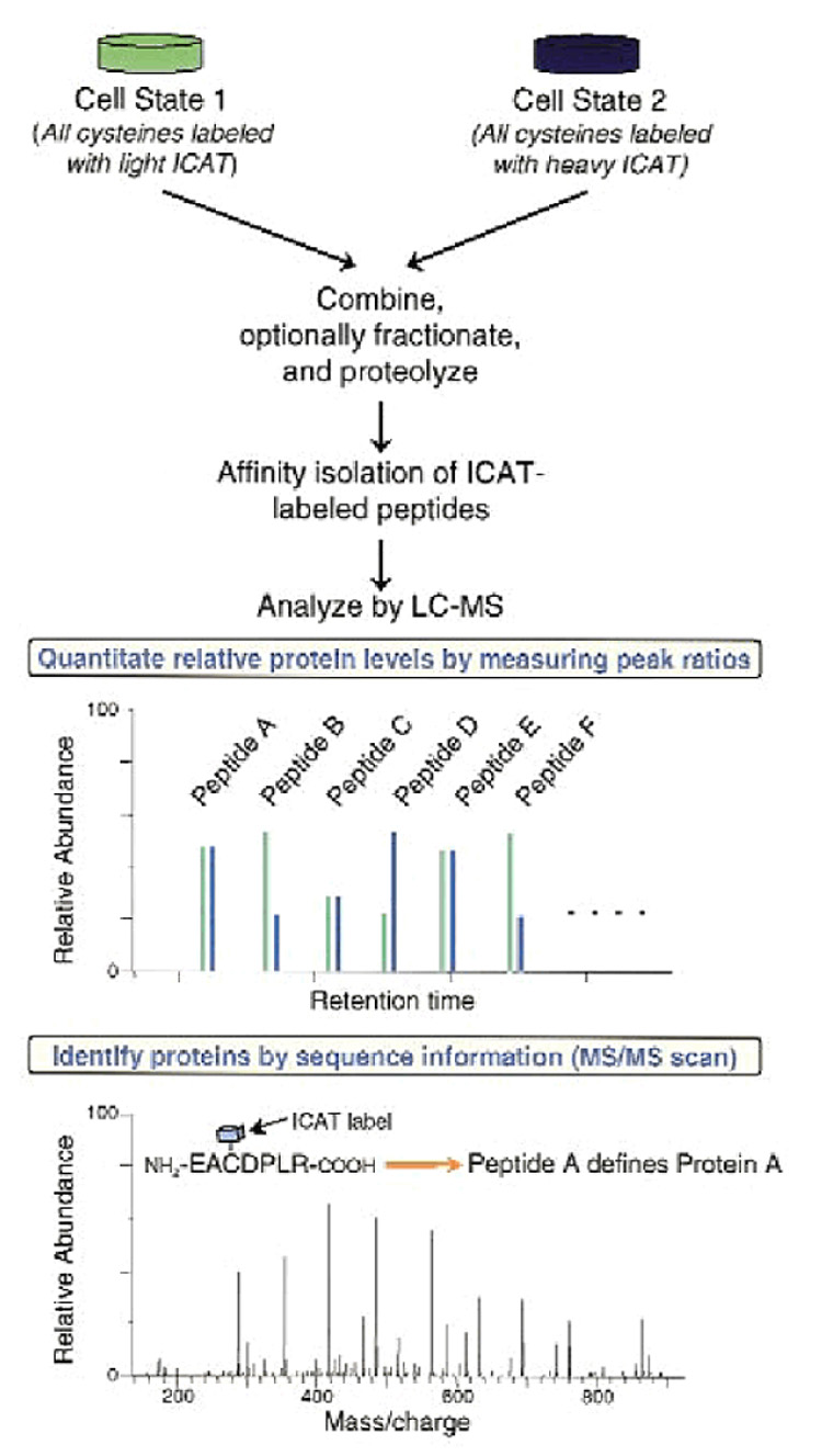
The ICAT strategy for quantifying differential protein expression. Two protein mixtures representing two different cell states have been treated with the isotopically light and heavy ICAT reagents, respectively; an ICAT reagent is covalently attached to each cysteinyl residue in every protein. Proteins from cell state 1 are shown in green, and proteins from cell state 2 are shown in blue. The protein mixtures are combined and proteolyzed to peptides, and ICAT-labeled peptides are isolated utilizing the biotin tag. These peptides are separated by microcapillary high-performance liquid chromatography. A pair of ICAT-labeled peptides are chemically identical and are easily visualized because they essentially coelute, and there is an 8 Da mass difference measured in a scanning mass spectrometer (four m/z units difference for a doubly charged ion). The ratios of the original amounts of proteins from the two cell states are strictly maintained in the peptide fragments. The relative quantification is determined by the ratio of the peptide pairs. Every other scan is devoted to fragmenting and then recording sequence information about an eluting peptide (tandem mass spectrum). The protein is identified by computer-searching the recorded sequence information against large protein databases. Reproduced from [65] with permission.

The value of the ICAT approach has now been demonstrated in numerous applications through its capability of quantifying proteins in complex mixtures. However, a relatively large size of the ICAT tag (~500 Da) limits database searching for small peptides. Another complication of this approach results from a common separation of the “heavy” and “light” pairs for the same peptide during LC, as the non-deuteriated peptides are retained longer than their deuteriated counterparts, causing variations in a precise isotope ratio determination. Since not all proteins contain Cys, roughly 15% of a typical proteome will not be covered through the ICAT approach.

B.1b. Global Internal Standard Strategy (GIST)

The abundance of reactive sites in a protein molecule permits utilization of isotope-labeling strategies besides the Cys-based ICAT approach. These approaches aim at labeling all peptides rather universally or “globally” [66–69] regardless of their amino acid composition. Due to their relatively uniform and frequent occurrence, arginine (Arg) and lysine (Lys) become the natural target of labeling strategies using different stable isotope reagents. The seemingly advantageous is a wide choice of derivatization and separation techniques to be employed in selection, identification and quantification of proteins.

One strategy involves the acylation of primary amino groups with either N-acetoxysuccinimide or N-acetoxy-[²H₃] succinimide [66,68]. Similarly to the ICAT determinations, the extracted proteome samples representing “experimental” and “control” are labeled with one of the two reagents prior to their mixing and proteolytic digestion. According to this approach, each peptide containing Arg at its C-terminus and a C-terminal Lys would be labeled doubly. Accordingly, an m/z difference of 3 or 6 will be observed for singly-and doubly-labeled peptides, respectively. Since virtually all peptides now carry a light/heavy label, the enormous complexity of this sample must be reduced through a variety of purification strategies.

GIST approach overcomes some limitations of ICAT. Since the mass increment due to tagging is very small, no variations in reactivity were reported, and a chromatographic separation of the heavy/light peptide pairs does not seem to occur. However, the procedure is still laborious and extensive sample handling is required in purifications, aiming to reduce sample complexity.

B.1c. iTRAQ™

As a major improvement over ICAT, a new labeling procedure, iTRAQ, has been developed by Pappin and co-workers at Applied Biosystems [70]. It involves a set of isobaric, amine-specific reagents, allowing a simultaneous identification and quantification for up to four different proteomes. This procedure is based on tagging the N-terminus of peptides generated from different protein digests with isobaric tags. The differentially labeled samples are then combined, subjected to nanoLC and analyzed by tandem MS. The following database searching of the MS fragmentation data readily identifies the differentially labeled peptides and hence the corresponding proteins. Due to the isobaric nature of the iTRAQ reagents, the same peptide from each sample pool appears as a single peak in the MS spectrum, thus reducing substantially spectral complexity. However, fragmentation of the tag attached to the peptides generates a low molecular mass reporter ion (at m/z 114.1, 115.1, 116.1, and 117.1) that is unique to the tag used to label each of the four digests (Figure 9). The intensity measurements of these reporter ions enables quantification of the respective peptides in each digest and hence the proteins from which they originate.

Figure 9.

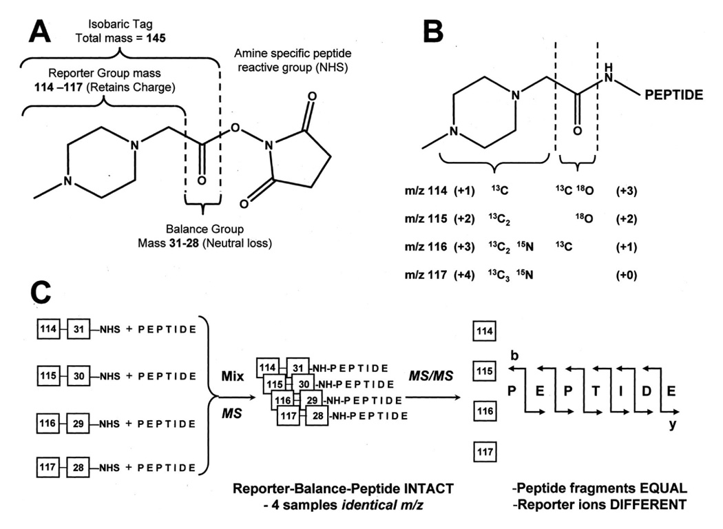
Diagram showing the components of the multiplexed isobaric tagging chemistry (A). The complete molecule consists of a reporter group (based on N-methylpiperazine), a mass balance group (carbonyl), and a peptide-reactive group (NHS ester). The overall mass of reporter and balance components of the molecule are kept constant using differential isotopic enrichment with ¹³C, ¹⁵N, and ¹⁸O atoms (B), thus avoiding problems with chromatographic separation seen with enrichment involving deuterium substitution. The number and position of enriched centers in the ring has no effect on chromatographic or MS behavior. The reporter group ranges in mass from m/z 114.1 to 117.1, while the balance group ranges in mass from 28 to 31 Da, such that the combined mass remains constant (145.1 Da) for each of the four reagents. B, when reacted with a peptide, the tag forms an amide linkage to any peptide amine (N-terminal or amino group of lysine). These amide linkages fragment in a similar fashion to backbone peptide bonds when subjected to CID. Following fragmentation of the tag amide bond, however, the balance (carbonyl) moiety is lost (neutral loss), while charge is retained by the reporter group fragment. The numbers in parentheses indicate the number of enriched centers in each section of the molecule. C, illustration of the isotopic tagging used to arrive at four isobaric combinations with four different reporter group masses. A mixture of four identical peptides each labeled with one member of the multiplex set appears as a single, unresolved precursor ion in MS (identical m/z). Following CID, the four reporter group ions appear as distinct masses (114–117 Da). All other sequence-informative fragment ions (b-, y-, etc.) remain isobaric, and their individual ion current signals (signal intensities) are additive. This remains the case even for those tryptic peptides that are labeled at both the N terminus and lysine side chains, and those peptides containing internal lysine residues due to incomplete cleavage with trypsin. The relative concentration of the peptides is thus deduced from the relative intensities of the corresponding reporter ions. In contrast to ICAT and similar mass-difference labeling strategies, quantitation is thus performed at the MS/MS stage rather than in MS. Reproduced from [70] with permission.

The iTRAQ approach seems to provide a substantial improvement over the other chemical labeling strategies in terms of procedural complexity and uniform coverage of studied proteomes. The unique isobaric nature of the four available reagents doubles the throughput of differential investigations of proteomes, while no chromatographic separation of the differentially tagged peptides has been observed with these reagents. While quantification is based on tandem MS rather than primary MS data, the instrument duty cycles are especially challenging for low-abundance proteins. However, the reported results [70–73] indicated enhanced signals due to isobarically-tagged peptides, resulting in detection of a greater number of peptides per protein with high confidence as well as a better performance with low-abundance proteins.

While the chemical labeling proteomic strategies have evolved in sophistication and concept with the capabilities of modern LC-MS, from the point of view of biomarker discovery, the needs for higher throughput are still formidable. Devising the better ways for selective fractionation of various proteomes prior to proteomic measurements will not improve the throughput situation, but they are likely to enhance the quality of quantitative measurements, as it has already been seen in the case of serum and plasma depletion of the most abundant proteins [74,75] and fractionation with lectin chromatography [76–81].

B.2. Stable Isotope Labeling by Amino Acids in Cell Culture (SILAC)

SILAC was first introduced to proteomic studies several years ago [82,83]. It has been commonly referred to as “metabolic stable-isotope labeling”, which is essentially a time-honored biochemical approach. SILAC involves growing two populations of cells, with one in a medium containing a “light” (normal) amino acid, and the other in the medium that contains a “heavy” amino acid. “Heavy” amino acids may contain ²H, ¹³C and ¹⁵N. Incorporation of the “heavy” residue into a peptide results in a known mass shift relative to the peptide containing a “light” residue (Figure 10). Using ¹³C₆-Arg as such an amino acid, for example, will result in a 6 Da shift in the molecular weight of a peptide possessing one Arg residue.

Figure 10.

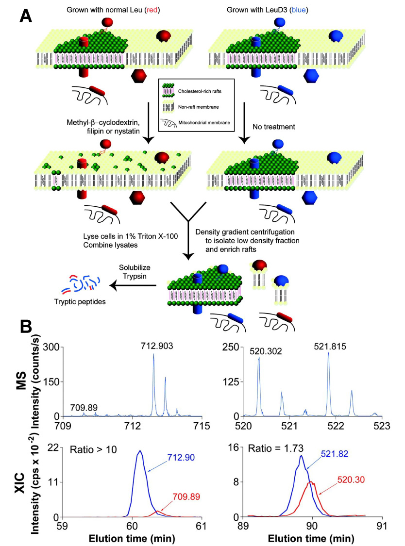
SILAC isolation scheme (A). Leu-labeled HeLa cells (depicted by red proteins/peptides) were treated with a cholesterol-disrupting agent, lysed, combined with lysates of LeuD3-labeled untreated HeLa cells (depicted by blue proteins/peptides), and used to prepare a detergent-resistant fraction. Because rafts in the drug-treated cells have lost their structural integrity, they no longer are purified in the detergent-resistant fraction, whereas nonraft contaminants originating from treated and untreated samples will copurify. Tryptic peptides were then prepared from isolated detergent- or pH/carbonate-resistant fractions MS and chromatograms (B). Representative MS and extracted ion chromatograms (XIC) for peptides from flotillin 1 and β-tubulin, two proteins identified in this study. Multiply charged peptides observed in MS mode were selected for fragmentation (MS/MS). Ion chromatograms (intensity vs. time) of Leu- and LeuD3-containing peptides identified by MS/MS were extracted from the series of MS scans and integrated by using SPINX (SILAC Peptide INtegration by XIC). Reproduced with modification from [83] with permission.

SILAC is apparently a “clean” procedure, which does not suffer from the problems of chemical labeling such as incomplete derivatization and formation of side-products. It offers high sensitivity without the need for sample purification. SILAC is suitable for studying the simple biological systems and changes associated with their perturbation.

B.3. Label-free Quantification

Numerous research laboratories now seem to explore different alternatives to isotopic labeling in proteomic studies. The procedures now commonly referred to as “label-free protein quantification techniques” have been based on either (a) relative quantification through a comparison of the number of peptides identified through LC/MS-MS; or (b) extracted ion chromatograms from LC/MS runs.

B.3a. Quantitative Proteomics-Based on the Number of Detected Peptides (Subtractive Proteomics)

The so-called “subtractive proteomics” is based on comparing the number of peptides identified for the same protein in different samples. The proteome, in this approach, is conventionally extracted from biological samples and then subjected to proteolytic digestion. The digested samples are then analyzed using multidimensional chromatography interfaced to an MS instrument, performing data-dependent tandem MS analyses. The relative abundance of a protein is simply related to the number of peptides identified for a specific protein in the samples under comparison. For example, protein X is 4-times more abundant in sample A relative to sample B, if the number of peptides determined for this protein is 4-times higher in sample A. This method is based on the assumption that the number of unique peptides identified for a particular protein is directly dependent on its abundance in the sample.

The major advantages of this approach are its inherent simplicity and small amounts of sample needed for analysis. However, to ascertain good sensitivity, a sufficient number of peptides must be detected for a protein in a very complex digest mixture. This, in turn, necessitates the use of two-dimensional chromatography, decreasing substantially analytical throughput. This approach is also totally dependent on the duty cycle of the MS instrument in use, and its capability of picking the same precursor ion in different samples that are subjected to tandem MS analysis and a subsequent database searching and identification.

B.3b. Quantitative Proteomics Based on Extracted Ion Chromatograms

This approach is based on the premises that the peak areas of peptides observed in an LC/MS analysis of a tryptic digest of a sample should correlate with their concentration. The peak areas of peptides originating from one protein as a result of proteolytic digestion should correlate with the concentration of that particular protein under identical LC/MS conditions. In this approach, proteomes are once again extracted from samples and proteolytically digested. The digested samples are then subjected to an LC/MS-MS analysis. Protein identification is achieved by correlating the tandem MS data with peptide sequences through database searching. The peak areas of identified peptides for a protein are then added to define the total reconstructed peak area of the protein digest.

The following assumptions apply for this approach: (1) the samples included in the study are largely similar to each other with respect to their peptide content (i.e., proteins from which these peptides originate are the same); (2) the same chromatographic conditions with acceptable reproducibility are employed during the analysis of all samples; and (3) the MS performance is identical for all analyses. The first assumption is totally dependent on the reproducibility of sample preparation, including proteolytic digestion, while the second and third assumptions are related to performance of both LC and MS parts, respectively. Several studies proposed the use of an internal standard prior to sample preparation [84,85] to offset the limitations of these assumptions.

Although several studies have demonstrated the importance of using an added protein or an endogenous protein as an internal standard [84,85] in normalizing the total reconstructed peak area of the protein digest, other studies have reported similar reproducibility and accuracy attained without the use of an internal standard [86–92]. In all cases, the obtained relative abundances, whether normalized or not, are quantitative within the MS dynamic range and become semiquantitative beyond it. Moreover, all studies have demonstrated a good reproducibility of the total reconstructed peak areas of protein digest (within 20% relative standard deviation) for highly complex proteomes. In general, more than 50%, and close to 90%, of the peptide area deviated less than 10% and 20%, respectively. This approach also demonstrated that the peak areas from LC/MS analyses correlate linearly with concentration of the protein (R² ≥ 0.95).

This approach is simple, requiring minimum sample preparation, in principle. However, reducing sample complexity through fractionation is still needed due to the limited dynamic range of MS with complex proteomes, limiting, once again, the analytical throughput.

While substantial progress has recently been made in proteomic quantification through LC/MS-MS procedures using ESI, the analysts must be periodically made aware of the ion suppression problems associated with this nearly routine ionization technique and interpret analytical data with caution.

5.2. GLYCOMIC PROFILING IN HEALTH AND DISEASE

Glycomic and glycoproteomic investigations can be counted among the most promising activities of the post-genomic era. Glycosylation of proteins is a wide-ranging and functionally important posttranslational modification. Many far-reaching medical consequences of the structural changes and metabolism of glycans are already known. Tentative connections of these versatile molecules have been made to congenital disorders, microbial infections, diabetes and cardiovascular problems, development of inflammation, toxicity effects, and cancer. Intimate knowledge of the disease-related changes of glycosylation patterns can potentially be integrated into the overall systems biology approach to provide far-reaching consequences for diagnostic applications, preventive medicine, and the development of novel therapeutic approaches.

While knowing the fine structural details on the whole biologically important glycoproteins is the ultimate long-term goal, it seems reasonable to assume that a wealth of practical information could be derived from quantitating the glycan patterns. Until recently, this area of investigation was somewhat limited by the lack of quantitative profiling procedures. Our laboratory has recently developed reproducible procedures for deglycosylation of proteins at microscale [93–95] that enable displaying the cleaved glycans into profiles that reflect the overall composition of physiological fluids and tissue extracts in terms of glycosylation (“normal” versus “aberrant”). The profiles can be displayed through different bioanalytical techniques: (a) MALDI-MS using a time-of-flight instrument [96] or an ESI mass spectrometer connected to capillary LC or capillary electrochromatography [97–99], or (b) capillary electrophoresis (CE), or (c) a chip-based separation using laser-induced fluorescence (LIF) detection. Each profiling approach assumes its own derivatization procedure, enhancing detection and a precise quantitative measurement.

Permethylation of glycans prior to an MS measurement has significant analytical merits due to such derivatives’ better ionization and fragmentation as well as the stabilization of sialylated (acidic) oligosaccharides. However, until recently [100,101], this time-honored derivatization technique of carbohydrate chemistry appeared unreliable for quantitative measurements due to incomplete methylation and degradation of some structures in the derivatization process. Consequently, a solid-phase permethylation of oligosaccharides in mixtures was developed at microscale [101] to overcome the quantitation difficulties of the previous procedures. In using MALDI-MS as the glycomic profiling approach, it has become feasible to include both the neutral and acidic glycans in one profile, as shown in Figure 11, which compares representative glycomic maps of a cancer patient to an individual free of the disease [102]. Importantly, these samples were derived from only 10-µL aliquots of human blood serum, demonstrating very high sensitivity of today’s analytical glycobiology. The sample treatment involved in these determinations has been currently optimized to process nearly two hundred sera, in parallel, during a 2-day period.

Figure 11.

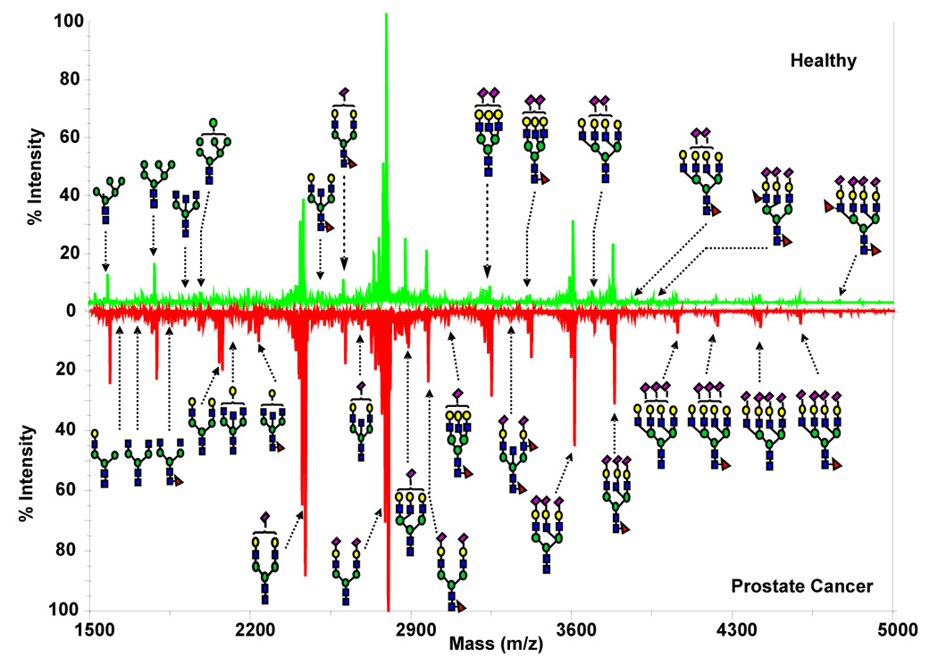
MALDI mirror spectra of permethylated N-glycans derived from human blood serum of a healthy individual vs. a prostate cancer patient. Symbols: , N-acetylglucosamine; , mannose; , galactose; , fucose; , N-acetylneuraminic acid. Reproduced from [102] with permission.

One of the inherent advantages of MS measurements is the capability to include stable-isotope labels for the sake of quantification. When methyl iodide is used as permethylation agent in our procedure, deuteromethyl iodide can be employed in running a comparison between normal and pathological samples in a single analytical run [103]. With a sufficiently high throughput and reliable quantification, as demonstrated in our recent studies [102,104], glycomic profiling procedures may even have a substantial diagnostic potential for different types of diseases.

Cancer is a set of diseases which has been for some time identified with the field of glycobiology [105–109]. During our recent studies on breast cancer [104], prostate cancer [102], liver cancer and other liver inflammatory disorders, we were able to analyze numerous blood serum samples and evaluate them statistically through different and independent chemometric procedures. The results of one of these comparisons are shown in Figure 12, where the principal component analysis clearly distinguishes different stages of cancer and clusters different patients’ glycomic profiles accordingly. In simple terms, the “biochemical individuality” of these patients, which is reflected in their averaged levels of different glycans (50–60 components determined per profile), has been changed from their “normal” state through different stages of the disease. How will different patients respond to their individual therapeutic regimes, as viewed through their glycomic profiles? Is there some biomarker change evident in the profiles of a person prior to acquiring distinct disease symptoms, i.e., occurrence of the primary tumor? These are some of the many questions that precise glycomic mapping could potentially provide answers for.

Figure 12.

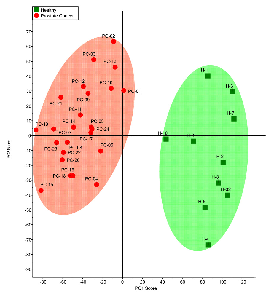
Principal component analysis (PCA) scores plot for mass spectra of glycans derived from blood sera of healthy individuals (n=10) and prostate cancer patients (n=24). Reproduced from [102] with permission.

A substantial limitation of biomedical MS in glycomic profiling is its weakness to distinguish many oligosaccharide isomers that the biological mixture may contain due to different sugar linkages, branching patterns, or a residue position on a particular antenna. Although we have recently demonstrated that high-energy tandem MS spectra reflecting cross-ring fragmentations are somewhat distinct [110,111] for different isomeric structures, it is difficult to do such measurements without prior isolation of these glycans or an on-line separation. One of the few techniques that can distinguish various sugar isomers at high measurement sensitivity is capillary electrophoresis (CE) [112–116]. While the glycans of interest must be tagged at their reducing end with a fluorophoric group to ensure detection through laser-induced fluorescence (LIF), the differences in hydrodynamic radius during electromigration in CE are still sufficient to distinguish different isomeric structures as distinct peaks [112–116].

An example of a CE/LIF glycomic profile is shown in Figure 13 with the fraction of an N-glycanase digest from human serum. Once again, the sample complexity reflected in this electropherogram suggests a source of potentially diagnostic information, but comparison of the relevant profiles on statistical basis is as yet incomplete. A minor disadvantage of a CE-based profiling is a relatively long analysis time (around 30-min duration), which can be overcome by a transfer of this analytical approach to a microchip format, as Figure 14 indicates. However, the problem of solute identification must await a development of reliable technologies for coupling such separation systems to MS. Multiplexing of the separate CE runs on a microchip for an enhanced analytical throughput is also a distinct possibility in future studies.

Figure 13.

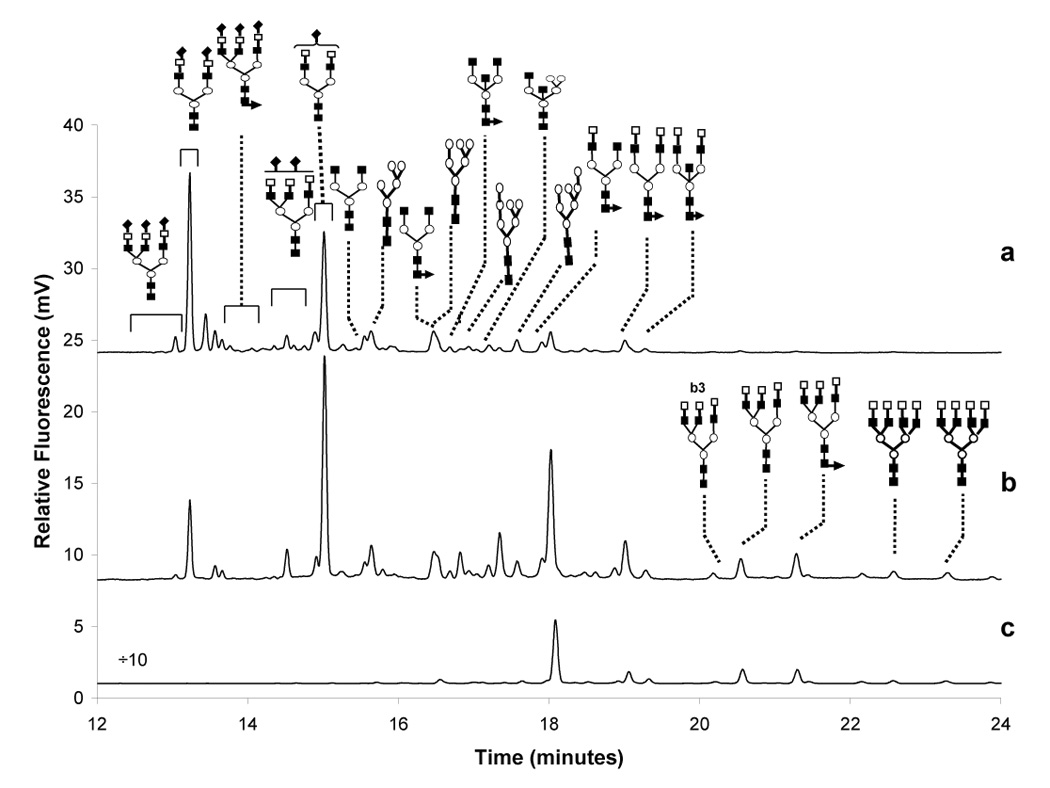
Electropherograms of N-glycans released from (a) human blood serum, (b) treated with 2–3 sialidase and (c) treated with 2–6 sialidase. Conditions: 60 cm acrylamide coated column (60 cm total length), 25 µm ID; LIF detection: argon-ion laser, excitation: 488 nm, emission: 520 nm; separation buffer: 40 mM Tris-HCl (pH 6.5), E=333 V/cm; 22.5° C. Symbols: □, galactose (Gal); ○, mannose (Man); ■, N-acetylglucosamine (GlcNAc); ▲, fucose (Fuc); and ♦, N-acetylneuraminic acid (NeuAC). Reproduced from [117] with permission.

Figure 14.

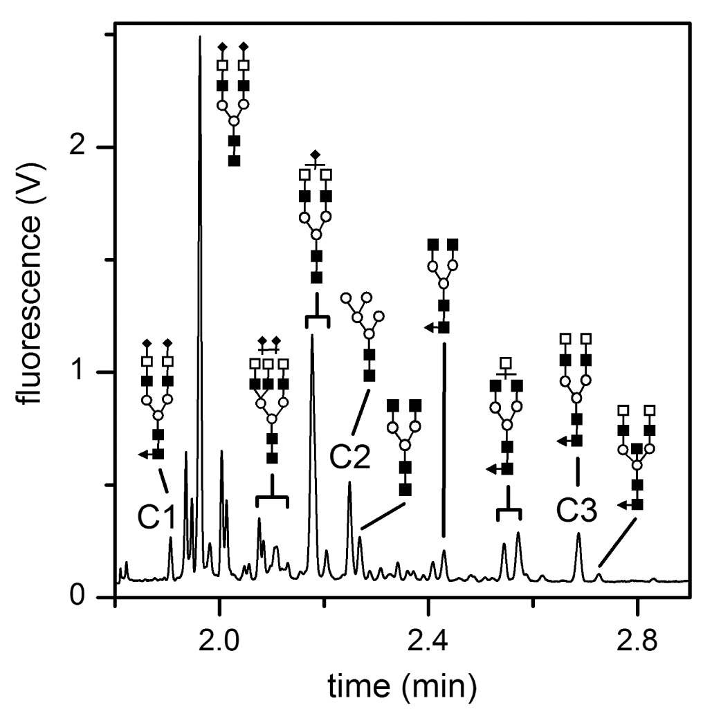
Electropherogram of N-glycans released from a blood serum sample from a stage IV breast cancer patient separated on the microfluidic device. The separation length was 22 cm, and the separation field strength was 750 V/cm. The separation efficiencies for components C1, C2, and C3 are listed in Table 2. Symbols: □ for galactose (Gal), ○ for mannose (Man), ■ for N-acetylglucosamine (GlcNAc), ▲ for fucose (Fuc), and ♦ for N-acetylneuraminic acid (NeuAC). Reproduced from [118] with permission.

5.3. CONNECTIONS BETWEEN GENES AND METABOLITES

Understanding life processes in their structural and dynamic details is a daunting task. With the increasing availability of specialized molecular profiling techniques to the biological and biomedical laboratories, and the increased emphasis on cross-disciplinary efforts, there is a need to translate complex molecular data to a broader view of life’s complexity, its chronology and dynamic nature, biorhythms, synchronization, symbiotic relations, etc. [14,119]. How does one approach an important research area through systems biology? The answer to this will of course depend on the inclinations, orientation and research experience of the individual investigators. Biologists may start with a choice of appropriate model systems and develop increasingly into the molecular aspects of investigation through acquiring new tools and techniques. A chemist/biochemist may initially favor either his favorite class of compounds (proteins, carbohydrates, steroids, prostaglandins, etc.) or a profiling technique (GC, LC, MS, etc.). Obviously, one starting point toward a productive investigation may start with the acquisition of complex molecular profiling data and explore certain correlations between the measured biochemicals toward building and describing a network for an appropriate biological model. To this date, modeling efforts in this area have been rare.

The “omics revolution” resonates with the Central Dogma of biology, giving genes the key role in life processes, with the current emphasis going from genotyping to phenotyping. However, as expressed appropriately by van der Greef and Smilde [120], “one cannot study a system by studying the building blocks only,” so that investigating molecular details of the phenotype, including its metabolome part, becomes essential. Empowered with the genomic knowledge of key organisms, the field of systems biology will increasingly move into measuring transcripts, proteins and their posttranslational modifications, as well as components of the complex metabolic networks.

A potential importance of connections between the genome and metabolome notwithstanding [2,121], there are relatively few and tenuous documented cases in the literature. Among the simplest systems to study a dynamic nature of the phenotype are microorganisms with a relatively easy system perturbation. Metabolomic studies and modeling will be considerably more difficult with the mammalian systems of a much greater organizational complexity of numerous cell types, cellular aggregations, and compartmentalization of different metabolic pools and pathways. Moreover, human studies are largely limited to the availability of physiological fluids, and seldom, small tissue biopsies.

Laboratory rodents, particularly the genus Mus domesticus (house mouse), have been bred for many generations as distinct strains with a well-defined genetic background. The more recent availability of genetic manipulation techniques provide further interesting possibilities for the wide use of laboratory mice in biomedical research. Through detailed metabolomic investigations, it is thus possible to compare the animals with different genetic background, including those with a single-gene deletion, and/or mutants within the same strain, against suitable controls. Among the biomedical applications of metabolomic procedures, these have been exemplified by the studies of db/db and db/+ mice (a maturite-onset diabetes model) through the GC-MS profiles of urinary acids and volatiles [122] as well as a more recent investigation of a transgenic ApoE3-Leiden mouse (atherosclerosis model) through NMR and LC-MS [123]. Moreover, congenic mice with the variations in the major histocompatibility complex (MHC) were found statistically distinguishable in their urinary volatile profiles [124–126].

Both the laboratory and wild mice represent very valuable animals for linking certain hormonal and behavioral attributes to their genetics. Mice use extensively a chemical communication system based on pheromones [33,127–129], primarily the volatile constituents of urine and glandular secretions. The pheromone components of a complex urinary profile recorded through GC-MS or other detection means are known to be involved in communicating the reproductive status, dominance and aggression [35] to a signal recipient within the species. Mice have been referred to as the reproductively most successful mammals on Earth, while their sophisticated chemical communication systems are viewed as highly important in this success [130].

While the phylogeny of the wild mice is well established [131], there have been no studies that would precisely characterize their genetic differences in terms of behavior and chemosignaling. For example, two groups which differ substantially in their nesting behavior and breeding are Mus musculus domesticus (common house mouse, which has a polygamous mating system) and Mus spicilegus (mound-building mouse, which is monogamous). During recent investigations [132], we have observed some major molecular differences between the two male mouse groups (Figure 15): the key pheromone of the house mouse, 2-sec-butyl-4,5-dihydrothiazole [133] is missing in the urine of M. spicilegus, while a different set of oxygenated volatiles, which are also under testosterone control, appear within the complex GC-MS profile.

Figure 15.

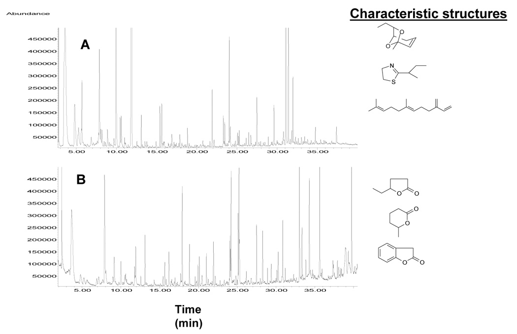
Comparative male mouse urinary volatile profiles for (A) Mus domesticus and (B) Mus spicilegus by GC-MS with characteristic chemical structures. Reproduced from [132] with permission.

It has been known for a long time that mating preferences in mice are related to certain regions of the MHC gene complex, yet not until recently [124–126], any biochemical evidence has been provided for this phenomenon. While mouse urine, a rich source of volatile constituents, is at least partially a source of this genetically-determined chemosignal, we have recently profiled the urinary samples of different MHC haplotypes, as exemplified in Figure 16. Our recent data from profiling a large set of potential chemosignaling compounds [126] provides evidence that even minute genetic variations in MHC can be reflected in the quantitative differences of selected metabolic profile constituents. Interestingly, some of these components include the previously identified pheromones [34]. Mus domesticus appears to be a suitable model for other gene-behavior studies, as some reports in the recent years suggest that MHC-dependent mating preferences may also be operative in fish, lizards, birds, and even humans [134].

Figure 16.

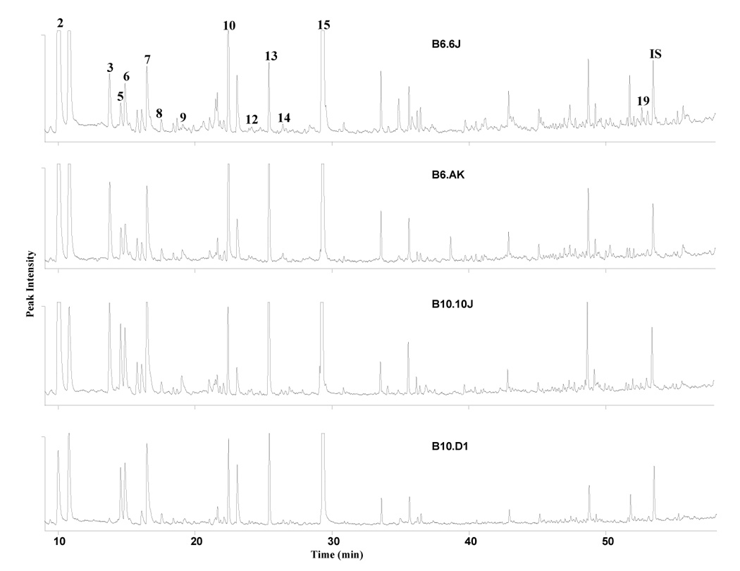
A comparison of male mouse urinary profiles measured by GC-AED carbon line 193 nm in different strains and haplotypes. Analysis conditions: capillary was HP-5MS (30 m × 0.25 mm, i.d., 0.25 µm film thickness) with the temperature program from 40° C (5 min) to 200° C at the rate of 2° C/min (10 min hold time). Numbers refer to compounds 2,3,7: dihydrofurans (DHF); 5: 2-heptanone; 6: 5-hepten-2-one; 8: 2-ethyl-5-methyl-5,6-dihydro-(4H)pyran; 9: 6-methyl-6-hepten-3-one; 10: 6-methyl-5-hepten-3-one; 12: limonene; 13: dehydro-exo-brevicomin (DHB); 14: acetophenone; 19: β-farnesene and IS: internal standard. Reproduced from [124] with permission.

A tentative relation of the human equivalent of the MHC genes to reproductive data [135,136] is supported by the fact that individuals have their distinctive scent, analogous to a “signature” or “fingerprint.” The individual odors can change due to a number of circumstances, such as menstrual cycle, emotional state, individual’s health, etc., yet each individual may retain their particular (genetically programmed) odor components. These, at least partially, explain that humans can recognize their own and their mate’s scents [137,138] and that mothers and their newborn infants mutually recognize each other through olfactory cues [139] When confronted with human scents, canines can readily distinguish individuals, but less so identical twins [140]. Mosquitoes are attracted variously to different individuals based on olfactory cues [141]. Body scent due to age and disease has also been discussed at numerous times.

While the body scent and volatile constituents were a subject of numerous studies in the past (for a review, see reference [142]), quantitative analyses and their statistical evaluations were not available due to a lack of suitable analytical techniques and a sufficient measurement throughput. We have recently developed a sampling approach [143], which permits quantitative evaluation of the skin volatiles sampled in a location remote from the analytical laboratory. This highly reproducible methodology has subsequently allowed us to participate in a cross-disciplinary study involving a repeated sampling of axillary sweat and physiological fluids from 196 adults living in a village in the Austrian Alps [144]. Their GC-MS samples were statistically analyzed chemometrically, yielding 373 chromatographic peaks that were consistent over time. Both individual and gender-specific chromatographic components were tentatively identified in their respective molecular profiles.

The examples of illustrative total-ion chromatograms from sampling of the axillary skin surface are given in Figure 17. Given the enormous complexity of repeated axillary sweat samples, no meaningful comparisons could be made without the measurement reproducibility [143] and the extensive use of chemometric procedures. The chemometric approaches used in our work [145,146] were, however, able to discriminate certain volatile components in terms of gender and family identification. Figure 18 exemplifies the multivariate nature of the data for the gender-specific marker compounds. A group of 14 compounds were determined to be marker compounds for sex as based on their abundance, although single compound square-rooted and normalized variations did not reveal the same property. Due to a general symbiotic relationship between humans and microorganisms, and more specifically, the perceived role of axillary microflora in human odor production [147,148], we used multivariate pattern recognition [149] in relating microbial genomic profiles with our GC-MS data. When the sampled subjects were divided into individual families, strong correlations were revealed, but some results must be interpreted with caution since such correlations might be influences by different personal behavior patterns in a family group.

Figure 17.

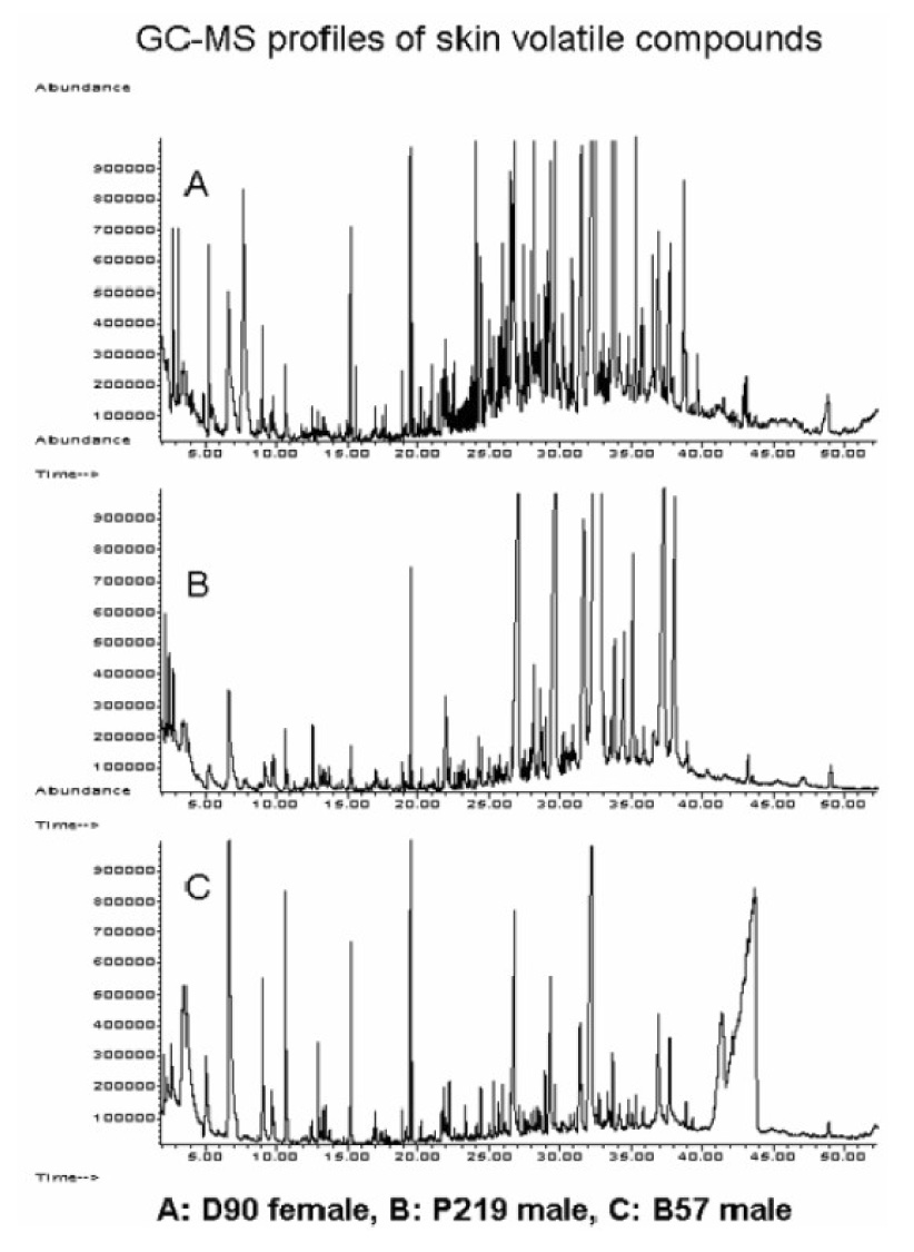
Representative human skin volatile profiles measured by GC-MS from different individuals within different families: A female (family D); B: male (family P); C: male (family B). Reproduced from supplementary data of [142] with permission.

Figure 18.

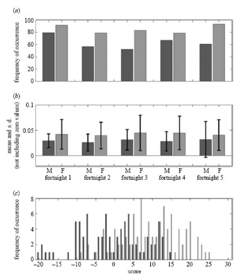
Distributions of markers that distinguish the sexes. (a) The distribution of the marker compound isopropyl hexadecanoate (RT 33.70 min), as the percentage of samples it was detected in and (b) mean and s.d. of the normalized squareroot intensity when detected in males and females, over all five fortnights. (c) Distribution of males and females is based on a model using the scoring system (black, male; grey, female). For each fortnight, if the male marker is detected in a specific individual, it is scored as K1, for a female marker it is scored as C1, so an individual scoring C35 contains the strongest possible female fingerprint, whereas an individual scoring K35 the strongest possible male fingerprint. Using a score of five as a divider between the classes, 75% can be correctly classified into their respective genders based on the presence and absence of 14 key markers. Reproduced from [142] with permission.

Dealing with the Complexity of Analytical Data

7.1. Bioinformatic Tools for Proteomic Applications

The success of any quantitative approaches relies heavily on the development of effective, reliable and user-friendly bioinformatic tools. As discussed previously, for the gel-based methodologies, quantitative evaluation will depend on aligning the gels and comparing the densities of the different gel spots. Differential densities under different excitation and emission wavelengths are employed in the case of DIGE, while the ratios of spots in different gels are used in the case of 2-DE. These bioinformatic tools capable of aligning and quantifying gel spots have been developed by the 2-DE and DIGE vendors. PDQuest 2-D Analysis Software developed by BioRad (Hercules, CA) organizes gels and quantifies the results. This software package normalizes each gel to “housekeeping proteins”, filters out background noise, and creates virtual gels using ideal Gaussian representations of experimental gels. In addition, this software allows statistical analysis of gels to determine which differences are significant and which are not. At each stage, PDQuest will show the spot of interest on all of the gels; sometimes, the user can make their own judgment call on whether the difference is significant or not. On the other hand, DeCyder™ Differential Analysis Software by GE Healthy (Piscataway, NJ) has been specifically developed as a key element of the DIGE system. DeCyder Differential Analysis Software automatically detects, matches and analyzes protein spots in multiplexed fluorescent images, and is capable of giving routine detection of < 10% differences with > 95 % confidence. Statistical analysis is carried out on each and every difference.

Less effort has been invested by the vendors when it comes to quantitative proteomics based on LC/MS analyses. Here, the vendors focused their efforts on the development of protein and peptide identification tools rather than on the quantification of LC/MS-acquired data. Therefore, individual researchers have often developed various bioinformatic tools, allowing an automated data interpretation and evaluation of LC/MS and LC/MSMS data. Such tools have been commonly developed to quantify LC/MS data, but they all also possess a component allowing protein identification.

A variety of algorithms, including SEQUEST, MASCOT, SpectrumMill and ProteinProphet have been developed to search raw MS or tandem MS data against different protein databases. Each algorithm offers its own advantages and disadvantages, yet they all allow the identification of proteins and peptides. Generally, the choice of one algorithm over the other is mainly based on personal preferences of any given laboratory.

Thus far, the bioinformatic tools developed for protein and peptide quantification adopt one of the two approaches. The first is based on the identification of peptides and proteins through LC/MSMS analysis, followed by quantification of peptides and, subsequently, their corresponding proteins. The second approach is more global in its nature, focusing on comparing all ions observed in an LC/MS analysis through various statistical tools such as support vector machines, decision trees, principal component analysis, and genetic algorithms. Such analyses result in creating a list of ions, enabling segregation of the two compared samples or sets of samples.

7.2 Chemometric Approaches to Metabolomics

While the extraordinary molecular complexity of biological mixtures is increasingly revealed by high-efficiency techniques and their connections to mass spectrometers and selective detectors, the use of chemometric procedures assumes particular importance. With hundreds of components resolved in a typical GC-MS and LC-MS runs, such data analyses can already be difficult due to the needs to identify and quantify all major and minor mixture components. When we add the high throughput of modern analytical procedures and a need to analyze many samples statistically in a typical biomedical or epidemiological study, the data handling and interpretation problem escalates rapidly. For a recent study involving GC-MS analysis of 196 individuals [144], each sampled repeatedly five-times, Dixon et al. [145] estimated that it would take nearly 19 years of full-time manual work to go through these human profiles. Fortunately, today’s fast computational techniques and modern chemometric procedures make such studies considerably easier.

Since our laboratory first advocated and used the pattern recognition approach for metabolic profiling and other complex chromatographic separations [28–30,150], there has been substantial progress with different chemometric approaches [151]. While the computational tools for multivariate non-linear statistical analyses became quite sophisticated, there are still special problems of pattern recognition compounded by large data sets. For example, for GC-MS and LC-MS data, total-ion chromatograms typically contain a very large number of peaks with varying intensities, which, moreover, frequently co-elute with other solutes, resulting in distorted spectra.

Successful pattern recognition procedures typically involve efficient data preprocessing methods [152]. Such methods can utilize peak-picking [153,154], followed by peak alignment algorithms [155–157]. Subsequently, the peaks can be normalized by summing the peak areas to a constant value in the sample, avoiding the skewing impact from the large peaks diminishing the importance of minor components (signals). Even appropriately organized raw data still require substantial processing if the number of variables is not reduced by defining those with the highest impact on the data sets. Naturally, a prior experimental/empirical knowledge of some variables can help reducing the numbers used for comparisons. Yet another means to simplify the data sets is to use Bayesian statistical methods to locate the signals with the highest impact on differences among the data sets [120].

In a simplified view, both metabolomic and proteomic analyses can produce a number of data sets which create a data matrix X(I × J), where I is the number of subjects and J number of variables. After the initial data organization steps, the commonly used pattern recognition tools currently involve principal component analysis (PCA) [158,159], principal component –discriminant analysis (PCDA) [160], or partial least squares (PLS) [161], and partial least squares discriminant analysis (PLS-DA) [162,163]. The PCA analysis creates score plots visualizing the relations between the subjects and loading plots classifying the relations between the measured variables. Such scatter plots can be difficult to interpret when there are large numbers of variables present [120]. The subsequently applied discriminant functions that are used for reduction of the number of variables simplifying the data classification as scatter plots [160]. PLS-DA methods have been used efficiently as classification and discrimination tools for processing very large data sets with a reduced number of variables.

Extensive metabolomic data may include added degrees of complexity, such as within-subject and between-subject variabilities. Multi-level batch statistical processing had to be used in modeling of urinary NMR data [164]. Another source of added complexity is a continuous change of the data input within time. In such cases, data analysis requires time-resolved or longitudinal data analysis approaches, such as the newly developed ANOVA-simultaneous component analysis (SAC) or ASCA. In this approach, the SCA models are built for each type of variation to facilitate easier interpretation of the variation from different factors of an experimental design [165].

Attempts have been made to use the entire metabolomic data to interpret fingerprints for the plant biophysical system [166]. Pair-wise correlations from the metabolomic data were used to create a metabolomic correlation network for interpretation of system’s fingerprints. However, a metabolomic correlation network would be a more challenging task in the case of mammalian systems, since the degree of biocomplexity exceeds that in the plant systems due to a wider occurrence of symbiotic microorganisms [15].

8 Conclusions

The most formidable challenges of biochemical complexity in the living systems are being gradually met through advances in bioanalytical chemistry. The recent availability of genomic tools has provided impetus to look into different aspects of phenotypic expression, particularly the proteomes, glycomes and metabolomes. The bioinformatic expansion of the recent years is a further essential means to deal with the enormously large data sets generated through high-resolution molecular profiling. The databases and database searches have been increasingly available for the field of proteomics, but similar efforts in glycomics and metabolomics are still in their infancy. While the available computer-aided identifications may provide encouraging “hints,” the identifications must still be considered tentative at best, or “hypotheses” that need further verification through the availability of standard, authentic glycans or metabolites, or in the area of proteomics, the proofs through targeted Western blots. Unequivocal structural identification deserves no less. The field of systems biology provides the common denominator for all different areas pertaining to biocomplexity.

Separation science and mass spectrometry have played enormous roles in unraveling the molecular attributes of life since the early concepts of “biochemical individuality” and “metabolic profiling” formulated during the 1960s. The emphasis on coupling the best separation tools with mass spectrometry, as they gradually develop, remains with us to this date. As the GC and GC-MS-based methodologies have now matured to the stage of routine utilization on the automated basis, they become very valuable assets of today’s metabolomics together with the other obvious choices, such as LC-MS and NMR spectrometry.

After a slow rate of acceptance during the 1980s, miniaturized (capillary) separations in the liquid state, i.e., capillary LC and CE, are becoming the common techniques in virtually all fields pertaining to systems biology. While their capabilities of handling effectively biomolecules at unprecedented low levels were demonstrated earlier, it was undoubtedly the “MS revolution” of the late 1980s and the arrival of new ionization techniques that gave nanoscale separations their new meaning. They are now incorporated routinely to all major analytical platforms for proteomics. The bourgeoning field of analytical glycobiology, which has often been neglected by the proponents of systems biology, relies on similar methodologies and instrumentation.

The recent emphasis in molecular profiling of biological materials has clearly been on improved quantification. Besides aiding the biomarker discovery and future diagnostic/prognostic uses of biomolecular profiling techniques, reliable quantitative methodologies will undoubtedly answer many additional questions of future research in biocomplexity.