Correction of B0-Susceptibility Induced Distortion in Diffusion-weighted Images Using Large-Deformation Diffeomorphic Metric Mapping

Abstract

Geometric distortion caused by B0-inhomogeneity is one of the most important problems for diffusion weighted images (DWI) using single shot, echo planar imaging (SS-EPI). In this study, large-Deformation, Diffeomorphic Metric Mapping (LDDMM) algorithm has been tested for the correction of geometric distortion in diffusion tensor images (DTI). Based on data from nine normal subjects, the amount of distortion caused by B0-susceptibility in the 3T magnet was characterized. The distortion quality was validated by manually placing landmarks in the target and DTI images before and after distortion correction. The distortion was found to be up to 15 millimeters in the population-averaged map and could be more than 20 millimeters in individual images. Both qualitative demonstration and quantitative statistical results suggest that the highly elastic geometric distortion caused by spatial inhomogeneity of the B0 field in DTI using SS-EPI can be effectively corrected by LDDMM. This postprocessing method is especially useful for correcting existent DTI data without phase maps.

1. Introduction

Diffusion tensor imaging (DTI) is an MRI technique that can visualize detailed white matter anatomy. Using this technique, various axonal bundles can be discretely identified. This opens up a new research area, with which we can assess the impact of various factors on the morphology of specific axonal bundles. For example, it is well known that white matter volume increases during brain development and decreases during aging. What we do not know is whether all axonal bundles increase or decrease their volumes proportionally during these processes. Or, under pathological conditions, are there specific bundles that experience atrophy? These findings would provide important clues about normal and abnormal brain formation and aging processes.

When we perform morphological studies using MRI, it is assumed that MRI has a high degree of fidelity to the actual brain anatomy. However, DTI, which is usually based on single-shot, echo planar imaging (EPI), contains image deformation due to B0-susceptibility differences over the brain. Fortunately, the degree of distortion has been dramatically reduced in recent years due to the introduction of parallel imaging [1, 2], although a certain amount of distortion still remains around the tissue-air interface.

Currently, there are roughly two types of post-processing methods for distortion correction. For the first method, a phase map or field map plays an essential role [e.g. 3–9]. While this is a viable option, precise measurement of the phase map is not straightforward and integration with parallel imaging would be challenging. The second approach is independent from imaging acquisition protocol. In this approach, EPI images are warped to co-register anatomical MR images, such as T₁/T₂-weighted images [e.g. 10–13]. The deformation process provides information about the location and the amount of distortion and the resultant transformed image will, in theory, provide distortion-free EPI images. For this purpose, we need to resort to non-linear image transformation (also known as elastic warping) because the image distortions are highly non-linear. When using non-linear transformation, the degree of elasticity can be controlled. For example, if polynomial fitting is used, the higher order polynomial allows the shape to be changed more freely. In the past, this type of post-processing could not provide satisfactory distortion corrections because the distortion in the SS-EPI was often too severe. In view of continuously improving image-matching technology and the recent introduction of parallel imaging that has drastically reduced the distortion, re-evaluation of the efficacy of nonlinear matching may prove useful.

Practically, with DTI more widely used in clinical studies, large amount of DTI data without phase/field map has already been acquired. Statistical analysis usually needs large samples. Sometimes the existent data which do not have phase map may constitute a big portion of the samples. Under this circumstance, recruiting patients and acquiring new data with phase/field map seems a more expensive way than making usage of the existent DTI data with distortion, if a nonlinear transformation can correct distortion effectively.

In this study, we tested a nonlinear warping algorithm based on large-deformation, diffeomorphic metric mapping (LDDMM) [14–16] to match images. LDDMM is an advanced, non-linear transformation method that enforces preservation of topology even with severe distortion. We applied this method to 3T DTI data acquired with parallel data acquisition. To evaluate the quality of distortion correction, manually defined anatomical landmarks were used to statistically quantify the distance errors. Distortion correction quality, advantages, and disadvantages of the proposed method are discussed. The proposed method with executable software available from the internet (http://www.cis.jhu.edu/software/lddmm-volume/index.html) will be especially useful for distortion correction of existent DTI data.

2. Brief Theory of Large-Deformation Diffeomorphic Metric Mapping

This section briefly describes theory of LDDMM method. Please refer to the literature [14–16] for details. The use of LDDMM to study the shapes of objects requires the placement of shapes in a metric space. It provides a diffeomorphic transformation (one-to-one, reversible smooth transformations that preserve topology), and defines a metric distance that can be used to quantify the similarity between two shapes. We assume that the shapes can be generated via a flow of diffeomorphisms, solutions of ordinary differential equations,

$$\frac{\partial {\phi }_t}{\partial t}=v_t({\phi }_t),t\in [0,1]$$ (1)

where φ_t are deffeomorphisms, φ₀ are identity maps that have ones at diagonal entries and zeros elsewhere, ν_t are associated velocity fields and t denotes time. For a pair of images, I_template and I_1, a diffeomorphic map φ₁ transforms one to the other

$${\phi }_1·I_{\mathit{template}}=I_1$$ (2)

at time t = 1. The metric distance between them is the length of the geodesic curves, φ_t·I_template t ∈ [0,1] through the shape space generated from connecting I_template to I₁ in the sense that φ₁· I_template,= I_1. The metric ρ(I_template,I₁) between I_template and I₁ takes the form

$$\rho {(I_{\mathit{template}},I_1)}^2=\underset{v_t:{\stackrel{.}{\phi }}_t=v_t({\phi }_t),{\phi }_0=id}{inf}{\int }_0^1\parallel L{v}_t\mid {\mid }^{2}dt$$ (3)

such that φ₁· I_template = I_1, where Lν_t are smooth vector fields with norm ||L·||. L is a linear differential operator to ensure that the solutions are diffeomorphisms. inf denotes infimum. For matching two images, L is chosen to be of the Cauchy-Navier type in the form of

$$L=-\alpha {\nabla }^2+\gamma id$$ (4)

where ${\nabla }^2=\frac{\partial }{\partial x^2}+\frac{\partial }{\partial y^2}+\frac{\partial }{\partial z^2}$ is the Laplacian operator and id is the identity operator [14]. The coefficient α enforces smoothness, large values ensuring solutions are diffeomorphic, and the coefficient γ is chosen to be positive so that the operator L is non-singular.

The metric ρ and the diffeomorphic map φ between I_template and I₁ are computed via a variational problem:

$$J(v_t)=\underset{v_t:{\stackrel{.}{\phi }}_t=v_t({\phi }_t),{\phi }_0=id}{inf}{\int }_0^1\parallel L{v}_t\mid {\mid }^{2}dt+D({\phi }_1·I_{\mathit{template}},I_1)$$ (5)

where D(φ₁·I_template, I₁) quantifies the closeness between the deformed image, φ₁·I_template, and target image, I_1. A gradient descent algorithm is used to seek an optimal solution for the above variational problem.

In practice, for distortion correction of DTI images, only α in equation (4) will be adjusted to determine the degree of elasticity and all other parameters can be used with their default optimal values. Detailed implementation can be found in section 3.3.

3. Materials and Methods

3.1. Data Acquisition and Preprocessing

The study was approved by Institutional Review Board (IRB) and informed consents including a HIPAA compliant data sharing agreement were obtained from all subjectes. Nine normal subjects (age 11–18, 4 male and 5 female) participated in this study. A 3 T Philips Achieva scanner was used for MRI scans. Human brain DTI data were acquired using a single-shot EPI sequence with a SENSE parallel imaging scheme (SENSitivity Encoding, reduction factor = 2.5). The imaging matrix was 96×96, with a field of view of 212 × 212 mm (nominal resolution of 2.2 mm), which was zero-filled to 256 × 256. Axial slices of 2.2 mm thickness were acquired parallel to the anterior–posterior commissure line. A total of 60 slices covered the entire brain and brainstem without gaps. The diffusion weighting was encoded along 30 independent orientations [17] and the b-value was 700 sec/mm2. Five additional images with minimal diffusion weighting (b= 33 sec/mm2) were also acquired (called b0 images hereafter). TE and TR were 97ms and 11.8s, respectively. The acquisition time per dataset was approximately 6 minutes. To enhance the signal-to-noise ratio, imaging was repeated two times, resulting in total acquisition time 12 minutes. Co-registered T₂ weighted images, using a double spin echo sequence, were acquired with a first echo time of 40ms, a second echo time of 100ms, and a repetition time of 6,084ms. The T₂-weighted image was used for anatomical reference for distortion correction.

Different from distortion caused by B0-inhomogeneity susceptibility, there is distortion caused by eddy current due to big gradient changes in diffusion weighted image acquisition. Twelve-mode linear affine intra-subject registration was performed to correct eddy current distortion using automated image registration (AIR) [18] for all 30 diffusion-weighted images with average of 5 b0 image as reference [19].

3.2. Tensor Calculation

Six independent elements of the 3 × 3 diffusion tensor were determined by multivariate least-squares fitting of raw DWI images. The tensor was diagonalized to obtain three eigenvalues (λ_1–3 ) and eigenvectors (ν_1–3 ). Anisotropy was measured by calculating fractional anisotropy (FA) with equation below:

$$FA=\frac{\sqrt{{({\lambda }_1-{\lambda }_2)}^2+{({\lambda }_1-{\lambda }_3)}^2+{({\lambda }_2-{\lambda }_3)}^2}}{\sqrt{2}\sqrt{{\lambda }_1^2+{\lambda }_2^2+{\lambda }_3^2}}$$ (6)

The eigenvector associated with the largest eigenvalue (ν₁ ) was used as an indicator of fiber orientation. For color-coded orientation maps, red (R), green (G), and blue (B) colors were assigned to left-right, anterior-posterior, and superior-inferior orientations, respectively [20]. For the color presentation, 24-bit color was used, in which each RGB color had 8-bit (0–255) intensity levels. The unit vector ν₁ (= [ν_1x, ν_1y, ν_1z]) always fulfills the condition, ν_1x² + ν_1y²; + ν_1z² = 1. Intensity values of ν_1x²*255, ν_1y²*255, ν_1z²*255 were assigned to the R(ed), G(reen), and B(lue) channels, respectively. In order to suppress orientation information in isotropic brain regions, the 24-bit color value was multiplied by FA. Average diffusion-weighted images (aDWI) were obtained by adding all diffusion-weighted images.

3.3. Application of LDDMM to T₂-weighted image/b0 image Registration

The LDDMM registration procedure is summarized as follows:

1. T₂-weighted image and b0 image were skull-stripped.

2. The intensities of the T₂-weighted image and the b0 image were adjusted using a histogram equalization method [21].

3. Within each subject, the T₂-weighted image was used as the target image and the b0 image representing the DTI data was deformed to the target image using LDDMM algorithm. A two-step deformation process was conducted. In the first step, α in operator L (equation 4) was set at 0.01 to achieve global registration. More elastic transformation was performed by setting α at 0.002 in the second step. The transformation matrix obtained from LDDMM mapping was applied to the DTI images using tri-linear interpolation and a distortion map was computed.

The LDDMM mapping procedure was implemented with C code and run in a Linux platform workstation. The usage and parameter settings of this software can be found in the webpage http://www.cis.jhu.edu/software/lddmm-volume/manual.html.

3.4. Calculation of Distortion Map and Distortion Correction

After b0 images were transformed to the target T₂-weighted images, a distortion map was calculated. Although distortion could happen in both X (phase encoding) and Y (frequency encoding) orientations, only the Y component was visualized because it is usually much larger than the X component. For every pixel in the b0 image, its locations before (x_B=[x_B, y_B, z_B]) and after (x_A=[x_A, y_A, z_A]) distortion correction were obtained and a distortion map was calculated by x_B−x_A=[x_B−x_A, y_B−y_A, z_B−z_A]. Note that B0-inhomogeneity causes both elongation and shrinkage of the tissue and distortion map, which is a scalar map of (y_B−y_A), contains both positive and negative values consequently. The LDDMM matching was repeated for data from the nine subjects to characterize geometric distortion in each subject. For group analysis, the distortion maps were normalized to the ICBM-152 template (www.loni.ucla.edu/ICBM) using an affine transformation, and a group-averaged distortion map was created.

For distortion correction of diffusion tensor, the transformation matrix was applied to all diffusion-weighted images. A new diffusion tensor was fitted with the corrected DWIs with the method described in section 3.2.

3.5. SPM

An automatic registration method, SPM (Statistical Parametric Mapping) (22), was also tested for distortion correction. For a fair comparison, the following parameters were not default but had been optimized to correct highly localized distortion. As in LDDMM, skull-stripped T₂-weighted images and b0 images were used. Intensity histograms of these two images were matched prior to the normalization. In the “Normalize” module of SPM, the following parameters were used for “Estimation Options”: source image smoothing=0; template image smoothing=0; no affine regularization; nonlinear frequency cutoff=10; nonlinear iteration=16; and nonlinear regularization=5. The following parameters were used for “Writing Options”: preserve concentrations; bounding box=[−106, −106, −61.6; 106, 106, 61.6]; voxel sizes=[0.828, 0.828, 2.2]; tri-linear interpolation; and no wrap.

3.6. Assessment of Distortion Correction

To assess the quality of distortion correction, we manually placed eighty-one homologous landmarks in each of the b0 image, the corrected b0 image, and the corresponding anatomical T₂-weighted image for every subject. The landmarks were placed on the characteristic anatomical locations such as tips of ventricles, boundaries of sulci. Those locations can be easily and consistently identified. The rater was blind to correction status when placing landmarks. After the distortion correction using LDDMM or SPM, the eighty-one landmarks in every b0 image were transformed to the correspondent anatomical T₂-weighted image. The Euclidean distance between paired landmarks before and after distortion correction was computed and referred to as the distance error to quantify distortion error. Its cumulative distributions for every subject were generated for before and after LDDMM and SPM processing to represent the percentage of paired landmarks with a distance of less than d mm. We performed a one-sided Kolmogorov-Smirnov (KS) test on the distance cumulative distribution and hypothesized that there was no difference before or after distortion correction against the alternative that the LDDMM method significantly reduces distortion error compared to before distortion correction. The empirical distribution estimate of KS statistics was obtained using the permutation-based resampling approach to reduce the risk of a large number of degrees of freedom. The resampling was not performed independently and landmark-by-landmark, but rather, the entire eighty-one landmarks were resampled as a whole without replacement. For each resampled dataset, the KS statistic was recomputed. By repeating this process ten thousand times, an empirical null distribution of the KS statistic was constructed, and the P-value was computed as a percentage of the KS statistics greater than the KS value from the original dataset.

4. Results

4.1 Phantom Study

A digital phantom was created to visualize the deformation field and evaluate the quality of elastic warping with LDDMM. The results are shown in Fig. 1. The distorted image and the image free of distortion are shown in Figs. 1a and 1b, respectively. The digital phantom of distorted image has both local expansion at the anterior part and local shrinkage at the posterior part (Figs. 1a and 1c). The LDDMM transformations with two different elasticity parameter settings were applied to the distorted image Fig. 1a. Both transformations evidently corrected distortion, as proved by the subtracted images Figs. 1e and 1h. Image warping of different elasticity with α = 0.01 and α= 0.002 is revealed by deformation fields, as shown in Figs 1f and 1i. Figs 1f and 1i also clearly demonstrate that the topology of the image is well preserved under both conditions. Higher elasticity is achieved with smaller value of Laplacian operator α.

Fig. 1.

LDDMM registration on digital phantom with control of elastic warping. (a) is the image after local anterior expansion and posterior shrinkage of template image (b). (c) is the difference image of (a) and (b). (d) and (g) are the corrected results of LDDMM with α = 0.01 and α = 0.002, respectively. (e) is the difference image of (b) and (d) and (h) is the difference image of (b) and (g). (f) and (i) show the deformation field from LDDMM transformation.

4.2. Distortion Correction of 3T Human DTI Data

Figs. 2 and 3 show results of distortion correction of 3T DTI images using LDDMM and SPM. Fig. 2 is an axial slice from the acquired data and Fig. 3 is a reconstructed sagittal slice from all axial slices to give an overall view of distortion correction. The red and yellow curves indicate the boundaries of the brain and the lateral ventricles of the T₂-weighted image (Figs. 2a and 3a) using an intensity threshold. These boundaries are overlaid on the exact same locations of the b0 images and color-coded orientation map to serve as a geometric reference. Global distortion is easily appreciable in Figs. 2b, 2c, 3b, and 3c. To better reveal the localized distortion, dramatically distorted areas pointed by yellow arrows are magnified in Figs. 2h and 3h. After distortion correction by LDDMM, the red and yellow reference curves are well aligned to the corrected brain, shown in Figs. 2e, 2f, 3e and 3f. Specifically full correction at the elastically distorted areas in regions such as prefrontal lobe and the brainstem is evident from Figs. 2i and 3i. The distortion map is also shown in Figs. 2g and 3g, clearly indicating the spatial extent of the distortion. To unify orientation of the two-dimensional images, the slice locations in a three-dimensionally reconstructed brain are shown at the corners of Figs. 2–4.

Fig. 2.

The target T₂-weighted (a), uncorrected b0 (b), uncorrected color-coded (c), SPM-corrected b0 (d), LDDMM-corrected b0 (e), and LDDMM-corrected, color-coded (f) images. The color map shown in (g) is a distortion map and the color bar indicates the distortion values in millimeters. (h) and (i) are enlarged uncorrected b0 and LDDMM-corrected b0, respectively. Axial slices at the level of the genu of the corpus callosum are shown. Red and yellow curves were defined by the brain boundary (red) and the lateral ventricle (yellow) of the target image and were superimposed on other images at the exact same locations. Yellow and white arrows indicate severely distorted regions that could be fully corrected by LDDMM and the regions where LDDMM performs better than SPM, respectively.

Fig. 3.

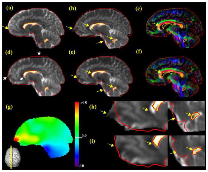
The target T₂-weighted (a), uncorrected b0 (b), uncorrected color-coded (c), SPM corrected b0 (d), LDDMM-corrected b0 (e), and LDDMM-corrected, color-coded (f) images. The color map shown in (g) is a distortion map. (h) and (i) are enlarged uncorrected b0 and LDDMM-corrected b0, respectively. The reconstructed para-sagittal slices from acquired axial images are shown to demonstrate the overall severe distortion at prefrontal lobe and pons. See legend of Fig. 2 for representation of red and yellow lines and that of yellow and white arrows.

Fig. 4.

Population-averaged 3D distortion map calculated from the nine subjects. Axial slices at the level of the internal capsule (a), the anterior commissure (b), the pons (c), the para-sagittal slice (d), and a coronal slice (e) are shown.

4.3. Averaged Distortion Map

Fig. 4 shows a 3D, averaged distortion map from the nine subjects imaged on a 3T scanner. The majority of the distortion is low-frequency (slow spatial change), and should be readily correctable by automated non-linear image matching routines. Severe (high-frequency) distortions are concentrated at the prefrontal lobe, the anterior edge of the brainstem, and the ventral temporal lobe. The amount of averaged distortion is smaller than that of the individual case shown in Figs. 2 and 3 because the severe distortions are localized in small regions and are not exactly at the same locations among different subjects.

4.4. Assessment of Distortion Correction

From Figs. 2 and 3, it can be seen that both LDDMM and SPM could correct distortion excellently. However, close inspection reveals some regions where LDDMM performed noticeably better (indicated by white arrows). To quantitatively assess distortion correction using different mapping methods, Fig. 5 shows the cumulative distribution of the distance error computed from the manually labeled eighty-one pairs of landmarks averaged across the nine normal subjects. The figure suggests that the distortion correction was improved with both SPM and LDDMM. However, LDDMM provides a better solution. The KS test shows that both correction methods statistically significantly corrected distortion compared to no correction (KS=0.4143, P<0.0001 for SPM; KS= 0.6214, P<0.0001 for LDDMM). Moreover, LDDMM statistically significantly corrected distortion compared to SPM (KS=0.2071, P<0.0001).

Fig 5.

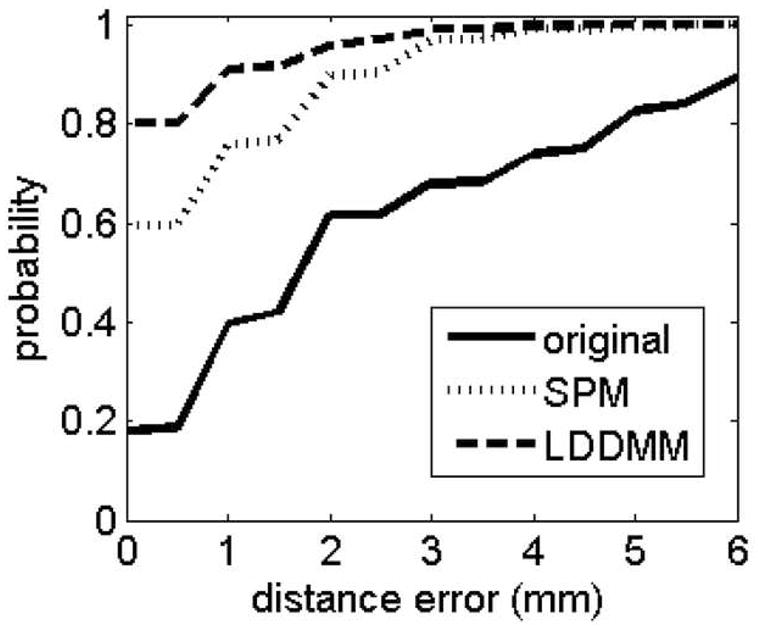
Cumulative distribution of distances between paired landmarks averaged across nine subjects. Solid, dot and dashed lines represent the distances before and after SPM and LDDMM distortion correction.

5. Discussion and Conclusion

We quantified the distortion in DTI datasets acquired with SS-EPI and parallel imaging acquisition. The characterization of distortion is especially important for DTI because DTI is often used for anatomical studies where it is important to maintain accurate sizes and shapes of anatomical structures. Currently, with DTI providing superb white matter structural information, most brain cortex anatomical information comes from conventional T₁/T₂ weighted images. Coregistration of images acquired from different imaging protocols by correcting the distortion is essential to fuse the anatomical information of total brain. As LDDMM is available from the internet, for researchers who do not have access to phase maps, distortion correction with LDDMM has proved to be an effective way. Due to its pure postprocessing characteristics, our method will be a useful remedy for existent data to get accurate anatomical information. To the best knowledge of authors, this study presents the first application of LDDMM to distortion correction of DTI data. In addition, SS-EPI is also widely used for other types of MRI studies, such as fMRI and, thus, our postprocessing approach could be useful for non-DTI studies.

In the past, distortion in SS-EPI was often beyond our ability to correct with satisfactory accuracy. Corrections based on a phase map or non-linear transformation can remove distortions to a certain degree, but these post-processing approaches have limitations if raw images have severe distortion. The introduction of parallel imaging was revolutionary, in the sense that it could reduce the distortion at its source. However, our study shows the displacement is still up to 15 millimeters in the population-averaged map and could be more than 20 millimeters in individual images after parallel data acquisition. The problematic distorted regions will greatly reduce the application of DTI since quite a few pathological states cause structural abnormality just within 15–20mm. Under these conditions, we can not tell if the abnormality/distortion results from imaging or diseases. Therefore, such distortion should not be overlooked and it is important to characterize and remove the substantial remaining distortions. Usually standard phase map measurement is a good solution to correct the distortion. With parallel imaging, the phase map measurement, however, is not straightforward and postprocessing is a more applicable method. In other cases when data was acquired and there is no possibility to recruit the subjects/patients to repeat the experiments, postproessing is the only choice. As expected, such distortions were concentrated around the regions of tissue-air boundaries, including the prefrontal lobe, the antero-ventral region of the temporal lobe, and the pons. It is important to point out that the distortion depends on many factors, such as magnetic field strength, gradient hardware quality, and image matrix size. Therefore, we cannot generalize our measurement results. Nonetheless, our results can be used as a reference for experiments with similar hardware and imaging parameters.

Roughly speaking, there are two types of distortion in SS-EPI images. One is low-frequency distortion, which refers to gradual anatomical distortion. This type of distortion was found throughout the brain in our study (Fig. 4), and could be easily corrected by the postprocessing image registration methods. The other type is high-frequency distortion, in which there is a sudden geometric transition from low to high distortion regions. In extreme cases, this leads to disappearance or collapse of signals from multiple pixels to a single pixel. Once this occurs, post-processing correction, including ours, cannot effectively correct the image. Other than these extreme cases, high frequency and localized severe distortion could be effectively corrected with the post-processing warping method. To avoid any inaccuracies due to the uncorrectable severe distortion, the distortion maps could be used as a binary mask to remove problematic regions (e.g., distortions larger than 10 mm) from the subsequent image analysis.

We compared LDDMM result with that of SPM. Although they both provide substantial improvement, LDDMM performed noticeably better. This is partly because LDDMM allows large deformation between two images. Furthermore, LDDMM generates the deformation velocity vector fields in the group of infinite dimensional diffeomorphisms, which is an elastic mapping method with a higher degree of freedom compared to SPM. However, we would like to stress that the matching quality depends on the parameter settings, and it is difficult to draw general conclusions from our study with regard to the software performance.

There are several disadvantages in the proposed approach. First, it requires a target image with very similar contrasts; in our case, a T₂-weighted image. Initially, we tried cross-contrast matching between T₁-weighted and DTI-derived contrasts. However, both LDDMM and SPM performed poorly. In this study, we used intensity-based cost functions and did not use mutual information. It would be an interesting future endeavor to determine whether satisfactory cross-contrast matching can be achieved by adapting a mutual information-based cost function. The second disadvantage is that the approach requires skull-stripping.

In conclusion, we tested LDDMM to measure and correct B0-related image distortion in SS-EPI with parallel data acquisition. Digital phantom study showed it corrected distortion with high elasticity while preserving topology. We further characterized and corrected distortions in DTI images acquired on a 3.0T scanner. Both qualitative observation and statistical evaluation show that LDDMM warping could correct localized and severe distortion with excellent quality. This postprocessing method has proved to be a useful tool for correcting distortion of existent DTI data. With the binary software available from internet, it can be used for distortion correction by DTI researchers without access to phase maps. The distortion map can be used to identify problematic regions and remove them from subsequent image analysis. This method, however, requires a non-distorted target image with similar contrast and skull-stripping.

References

- 1.Bammer R, Auer M, Keeling SL, Augustin M, Stables LA, Prokesch RW, Stollberger R, Moseley ME, Fazekas F. Diffusion tensor imaging using single-shot SENSE-EPI. Magn Reson Med. 2002;48(1):128–136. doi: 10.1002/mrm.10184. [DOI] [PubMed] [Google Scholar]
- 2.Pruessmann KP, Weiger M, Scheidegger MB, Boesiger P. SENSE: Sensitivity Encoding for Fast MRI. Magn Reson Med. 1999;42(5):952–962. [PubMed] [Google Scholar]
- 3.Jezzard P, Balaban RS. Correction for geometric distortion in echo planar images from B0 filed variations. Magn Reson Med. 1995;34(1):65–73. doi: 10.1002/mrm.1910340111. [DOI] [PubMed] [Google Scholar]
- 4.Reber PJ, Wong EC, Buxton RB, Frank LR. Correction of off resonance-related distortion in echo-planar imaging using EPI-based filed maps. Magn Reson Med. 1998;39(2):328–330. doi: 10.1002/mrm.1910390223. [DOI] [PubMed] [Google Scholar]
- 5.Chen NK, Wyrwicz AM. Correction for EPI distortions using multi-echo gradient-echo imaging. Magn Reson Med. 1999;41(6):1206–1213. doi: 10.1002/(sici)1522-2594(199906)41:6<1206::aid-mrm17>3.0.co;2-l. [DOI] [PubMed] [Google Scholar]
- 6.Cusack R, Brett M, Osswald K. An evaluation of the use of magnetic field maps to undistort echo-planar images. NeuroImage. 2003;18(1):127–142. doi: 10.1006/nimg.2002.1281. [DOI] [PubMed] [Google Scholar]
- 7.Andersson JL, Skare S, Ashburner J. How to correct susceptibility distortions in spin-echo echo-planar images: application to diffusion tensor imaging. NeuroImage. 2003;20(2):870–888. doi: 10.1016/S1053-8119(03)00336-7. [DOI] [PubMed] [Google Scholar]
- 8.Zeng H, Gatenby JC, Zhao Y, Gore JC. New approach for correcting distortions in echo planar imaging. Magn Reson Med. 2004;52(6):1373–1378. doi: 10.1002/mrm.20297. [DOI] [PubMed] [Google Scholar]
- 9.Chen B, Guo H, Song AW. Correction for direction-dependent distortions in diffusion tensor imaging using matched magnetic field maps. NeuroImage. 2006;30(1):121–129. doi: 10.1016/j.neuroimage.2005.09.008. [DOI] [PubMed] [Google Scholar]
- 10.Kybic J, Thevenaz P, Nirkko A, Unser M. Unwarping of unidirectionally distorted EPI images. IEEE Trans Med Imaging. 2000;19(2):80–93. doi: 10.1109/42.836368. [DOI] [PubMed] [Google Scholar]
- 11.Studholme C, Constable T, Duncan JS. Accurate alignment of functional EPI data to anatomical MRI using a physics-based distortion model. IEEE Trans Med Imaging. 2000;19(11):1115–1127. doi: 10.1109/42.896788. [DOI] [PubMed] [Google Scholar]
- 12.Andersson JL, Skare S. A model-based method for retrospective correction of geometric distortions in diffusion-weighted EPI. NeuroImage. 2002;16(1):177–199. doi: 10.1006/nimg.2001.1039. [DOI] [PubMed] [Google Scholar]
- 13.Ardekani S, Sinha U. Geometric distortion correction of high-resolution 3T diffusion tensor brain images. Magn Reson Med. 2005;54(5):1163–1171. doi: 10.1002/mrm.20651. [DOI] [PubMed] [Google Scholar]
- 14.Miller MI, Trove A, Younes L. On the metrics and Euler-Lagrange equations of computational anatomy. Annu Rev Biomed Eng. 2002;4:375–405. doi: 10.1146/annurev.bioeng.4.092101.125733. [DOI] [PubMed] [Google Scholar]
- 15.Beg MF, Miller MI, Trouve A, Younes L. Computing large deformation metric mapping via geodesic flows of diffeomorphisms. Int J Comput Vision. 2005;61:139–157. [Google Scholar]
- 16.Miller MI, Beg MF, Ceritoglu C, Stark C. Increasing the power of functional maps of medial temporal lobe by using large deformation diffeomorphic metric mapping. Proc Natl Acad Sci USA. 2005;102(27):9685–9690. doi: 10.1073/pnas.0503892102. [DOI] [PMC free article] [PubMed] [Google Scholar]
- 17.Jones DK, Horsfield MA, Simmons A. Optimal strategies for measuring diffusion in anisotropic systems by magnetic resonance imaging. Magn Reson Med. 1999;42(3):515–525. [PubMed] [Google Scholar]
- 18.Woods RP, Mazziotta JC, Cherry SR. MRI-PET registration with automated algorithm. J Comput Assist Tomogr. 1993;17(4):536–546. doi: 10.1097/00004728-199307000-00004. [DOI] [PubMed] [Google Scholar]
- 19.Mori S. Introduction to diffusion tensor imaging. Elsevier; 2007. [Google Scholar]
- 20.Pajevic S, Pierpaoli C. Color schemes to represent the orientation of anisotropic tissues from diffusion tensor data: application to white matter fiber mapping in the human brain. Magn Reson Med. 1999;42(3):526–540. [PubMed] [Google Scholar]
- 21.Gonzalez RC, Woods RE. Digital image processing. Upper Saddle River, New Jersey: Prentice Hall; 2001. [Google Scholar]
- 22.Friston KJ, Ashburner J, Frith CD, Poline J, Heather JD, Frackowiak RSJ. Spatial registration and normalization of images. Hum Brain Mapp. 1995;3:165–189. [Google Scholar]