Forecasting United States mortality using cohort smoking histories

Abstract

In this paper, we introduce a recently established relationship between cohort smoking patterns and adult mortality into mortality projections for the United States. In particular, we incorporate a variable representing the intensity of smoking within a cohort into the original Lee–Carter projection model. The introduction of this variable accounts for important anomalies in the recent age/sex pattern of mortality change and enables the use of a common temporal trend of mortality change for the 2 sexes. We project age-specific mortality rates for men and women at ages 50–84 between 2004 and 2034 in the United States. Because of reductions in smoking that have already occurred or can be reliably projected, mortality is projected to decline much faster when smoking is introduced into the model.

Cigarette smoking has long been recognized as a significant factor affecting human mortality (1). The effect of smoking on mortality is clearly visible in the mortality profiles of different birth cohorts in the United States (2). These cohort patterns offer an opportunity to add important information to mortality projections. In this paper we incorporate a variable representing the prevalence of smoking among cohorts into the Lee–Carter model, the most widely used model to forecast mortality. We demonstrate the effect of this incremental information on forecasts of American mortality.

Smoking and Mortality

Although epidemiologic studies have identified cigarette smoking as an important risk factor in mortality for at least a half century, there is no consensus on how great the risk is. The large studies that have garnered the bulk of attention are based on nonrepresentative samples and have typically recorded smoking status at baseline without changing the classification of individuals as their smoking status changes. Measurement error in smoking status has the effect of reducing the estimated risk. The two largest studies, each involving more than 1 million individuals, were conducted under the auspices of the American Cancer Society. Cancer Prevention Study I, conducted between 1959 and 1972, found a ratio of mortality among current smokers relative to never-smokers ages 40–84 of 1.91 for white men and 1.46 for white women (3). Cancer Prevention Study II found ratios of 2.52 to 2.82 for men between ages 50 and 79 during 1982–1996 and ratios of 1.33–1.89 for women at these ages (4). When adjustment for smoking cessation was made for a subsample for whom this information was gathered in Cancer Prevention Study II, the range of relative risks for current smokers rose to 3.11–3.53 for men and to 2.58–3.14 for women (4). This study also produced higher estimates of the long-term effects of smoking for those who had stopped. Rogers et al. (5) used a nationally representative sample and found risks for current and ex-smokers that are intermediate between the 2 Cancer Prevention Studies, controlling for education, family income, and a variety of other variables.

These studies show that the risk of death from smoking is high and endures many years after smoking has ceased. In view of the high percentage of the American population that consists of current or past smokers, a percentage that reached 77% in some male cohorts (3), it is not surprising that smoking has left a distinctive imprint on national mortality patterns. And in view of the enduring impact of smoking and its serial correlation across the life cycle, it is not surprising that much of that imprint is cohort-specific.

Smoking Patterns

The prevalence of cigarette smoking in the United States first rose and then fell in the course of the 20th century. However, the patterns were not the same for men and women (6). The sex differential in smoking prevalence also rose and fell, which was associated with widening and then narrowing sex differentials in mortality (2). Only about 6% of women smoked in 1924, a number that increased to 16% by 1929. However, during the same period, more than 50% of men smoked (6). For United States adults ages 18 and older, smoking prevalence was 56.9% for men and 28.4% for women in 1955. This sex difference of 28.5% subsequently declined to ≈5% and has remained there since the beginning of the 1990s. In this paper we rely upon a careful reconstruction of cohort smoking information for the United States that was done by Burns et al. (7).

Mortality Projections

There is no universally accepted method for projecting mortality. The methods that are used can be classified into 4 categories: projections by extrapolating age-specific mortality rates; projections by reference to a model mortality scenario; projections by interpolating current mortality and a targeted mortality in the future; and projections by reference to components of mortality (8).

There have been 3 major programs of mortality forecasting in the United States: projections by the Social Security Administration (SSA), by the Census Bureau, and a series of projections using a method developed by Lee and Carter (9). All of these programs are based on observations of past trends in period levels of mortality and assumptions about whether and how those trends will be modified in the future. The Census Bureau (10) uses Lee–Carter procedures to establish long-range targets to which estimates eventually converge. The Lee–Carter method has also been recommended by advisory panels to SSA for use by the SSA (11).

The Lee–Carter model (9, 12) has many advantages: it produces an excellent fit to mortality trends; it is parsimonious in the number of parameters used; it linearizes mortality trends and thereby adds confidence to extrapolations; and it produces sensible estimates of forecast uncertainty. The basic model can be expressed as

In this model, M_x,t is the central mortality rate for age x at time t, whereas a_x describes the mortality profile by age, which is constant over time; k_t represents the temporal trend of mortality changes over time; and b_x describes the changes in the mortality rates at age x in response to changes in k_t over time. The ε_x,t is an error term, which depicts the age period-specific influences that are not explained by the model. In the typical application, this model is fitted to past data to obtain parameter estimates, and projections are then made by holding the a_x and b_x parameters constant and extrapolating k_t.

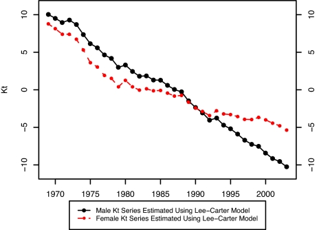
In their 1992 paper, Lee and Carter applied their model to the sex-combined United States population instead of applying it separately to male and female populations; they were concerned that extrapolating sex differentials in mortality would produce implausible differentials in the future. To illustrate the difficulty, we have estimated the Lee–Carter model separately for male and female United States populations between 1969 and 2003 at ages 40–84. Fig. 1 shows that the temporal trends in mortality are markedly different for males and females. In the past 35 years, male mortality has declined much more rapidly than female mortality, a pattern that may produce implausible results if projected far into the future.

Fig. 1.

K_t estimated by using the Lee–Carter Model: United States, 1969–2003.

Although cigarette smoking accounts for the highest number of “attributable deaths” of any physical risk factor in the United States (13), relatively few mortality projections have taken this factor into consideration. Pampel (14) forecasts sex differences in mortality in high-income countries while using data on smoking. Based on the relationship between smoking prevalence and lagged smoking mortality, he predicts a rapid decline of the logged ratio of male-to-female smoking-related mortality between the 1990s and 2020 for an aggregate of 21 developed countries. Bongaarts (15) indentifies mortality attributable to smoking and projects mortality assuming that component to be constant. Several national projection programs refer to smoking patterns as a basis for projecting narrowing sex differences in mortality (e.g., ref. 16).

The possibility that there is a strong cohort pattern in the relationship between smoking and mortality opens up promising new possibilities for mortality projection. A period-specific approach to smoking-based projections would require making predictions of smoking behavior at all ages for all future periods. In contrast, a cohort approach can rely primarily on cohort behaviors that have already been observed.

In this paper we incorporate a cohort smoking factor into the original Lee–Carter model to project mortality for the United States. We build on the Lee–Carter model by producing mortality forecasts jointly for males and females within the same model, rather than combining the two sexes or treating them individually. We use the average number of years spent as current smoker by age 40 as an indicator of smoking history for each cohort. This variable was successfully used to predict mortality by Preston and Wang (2). This variable is an indicator of smoking duration rather than of smoking intensity, which cannot be recovered from the retrospective data available. Studies of lung cancer mortality find that duration is a much more successful predictor than intensity (17).

Methods and Data

Model.

We assume that men's and women's mortality is influenced by age and period in the manner hypothesized by Lee and Carter, but that it is also influenced by smoking histories. In addition, we assume that males and females share a common temporal trend in mortality. The new model is:

In the above equations, a_x^Female and a_x^Male are the constant elements in the mortality profile by age for women and men, respectively; b_x^Female and b_x^Male describe the changes in the mortality rates at age x in response to changes in k_t over time for women and men, respectively; k_t is the level of mortality at time t, assumed to be the same for men and women when smoking histories are controlled; S_x,t^F and S_x,t^M are cohort smoking indices for women and men by single year and single age; and c and w are coefficients that indicate the effect of a particular smoking history on mortality of men and women, respectively. To reiterate, the differences between this modified Lee–Carter model and the original Lee–Carter model are that we introduce cohort smoking behaviors into the models and that men and women share a common mortality trend, k_t.

Eqs. 2.1 and 2.2 are then combined into a single equation for estimation purpose after a simple transformation as follows:

We can combine the above two equations into one:

We obtain Eq. 3 by simply stacking Eqs. 2.1.1 and 2.2.1 vertically. For example,

is a new matrix in Eq. 3 obtained by stacking matrices (ln (M_x,t^Female) − w·S_x,t^F) and (ln (M_x,t^Male) − c·S_x,t^M) vertically.

Eq. 3 can be estimated by singular value decomposition. In particular, we find a set of parameters that minimizes the sum of the squared errors, E, which is defined in the following form:

where

is the estimated matrix given c = c′ and w = w′. E is equal to sum of all of the squared elements in the error matrix, which is

Data.

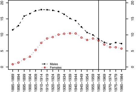
Mortality data are derived from the Human Mortality Database (www.mortality.org). The population data in this source are drawn from the U.S. Census Bureau. Data on deaths are taken from the National Center for Health Statistics. We use single-year of age mortality rates from ages 50 to 84 for every calendar year from 1969 to 2003. The first year for which we have complete smoking histories for all cohorts in the age interval under study is 1969. The cohort smoking index is reconstructed from the work by Burns et al. (ref. 7, with supplement supplied by the author), who relied on National Health Interview Surveys conducted between 1965 and 2001. We have converted the data into estimates of the average number of years that members of various birth cohorts smoked before age 40. We have assigned the smoking behavior for a 5-year birth cohort to each single-year birth cohort within that group. The value of the smoking variable for various birth cohorts of men and women is shown in Fig. 2.

Fig. 2.

Average number of years spent as a cigarette smoker before age 40 among men and women in different birth cohorts. Source: Preston S, Wang H (2).

Results

We solved simultaneously for all parameters, iterating across all possible values of c and w. The sum of squared errors was minimized by the set of parameters c′ = 0.031 and w′ = 0.017. A greater responsiveness of males to smoking is consistent with the epidemiologic studies reviewed above. In particular, Cancer Prevention Study I found that smoking raised male death rates by 91% and female rates by 46% (3), a sex difference very similar to that estimated here. Table 1 presents the estimated values of a_x^Male, a_x^Female, b_x^Male, and b_x^Female.

Table 1.

Estimated values of a_x and b_x for males and females

Age, yr	axMale	axFemale	bxMale	bxFemale
50	−5.4288	−5.7211	0.01233	0.01589
51	−5.3452	−5.6295	0.01157	0.01394
52	−5.2601	−5.5362	0.01263	0.01401
53	−5.1882	−5.4542	0.01287	0.01360
54	−5.1121	−5.3831	0.01457	0.01400
55	−5.0140	−5.2890	0.01437	0.01332
56	−4.9326	−5.1942	0.01451	0.01312
57	−4.8562	−5.1168	0.01544	0.01290
58	−4.7449	−5.0023	0.01459	0.01179
59	−4.6879	−4.9402	0.01546	0.01192
60	−4.5846	−4.8391	0.01595	0.01256
61	−4.5110	−4.7527	0.01461	0.01058
62	−4.4063	−4.6454	0.01514	0.01159
63	−4.3424	−4.5808	0.01522	0.01026
64	−4.2714	−4.5078	0.01518	0.01028
65	−4.1795	−4.4067	0.01596	0.01146
66	−4.1108	−4.3342	0.01527	0.01057
67	−4.0312	−4.2455	0.01571	0.01122
68	−3.9397	−4.1479	0.01538	0.01152
69	−3.8637	−4.0646	0.01568	0.01240
70	−3.7654	−3.9512	0.01666	0.01403
71	−3.6969	−3.8729	0.01503	0.01240
72	−3.5976	−3.7543	0.01637	0.01398
73	−3.5210	−3.6644	0.01577	0.01389
74	−3.4440	−3.5800	0.01623	0.01486
75	−3.3561	−3.4747	0.01680	0.01579
76	−3.2725	−3.3823	0.01633	0.01490
77	−3.1908	−3.2905	0.01599	0.01445
78	−3.1151	−3.1937	0.01544	0.01489
79	−3.0232	−3.0833	0.01586	0.01532
80	−2.9173	−2.9643	0.01680	0.01605
81	−2.8291	−2.8666	0.01550	0.01435
82	−2.7363	−2.7497	0.01614	0.01483
83	−2.6381	−2.6359	0.01582	0.01499
84	−2.5467	−2.5254	0.01618	0.01496

We have estimated Eq. 3 with and without data on smoking. The addition of the smoking variable explains 20% of the variance that was left unexplained by the Lee–Carter Model without smoking: the modified R² (i.e., the proportion of variance explained after age effects are accounted for) increases from 0.965 to 0.972. In addition, parameter values and projections are strongly affected.

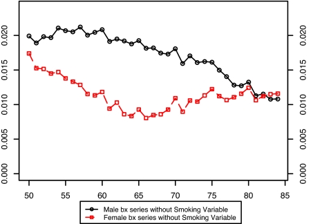
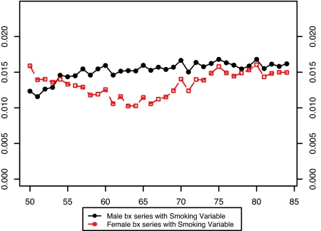
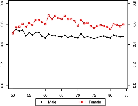
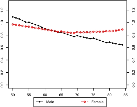
Fig. 3 presents the estimated values of the b_x for males and females without the smoking variable in the model. It is evident that there is a large disparity between the sexes in the estimated pattern of change in age-specific death rates when smoking is not included in the model. Furthermore, the age pattern of change is irregular for both sexes. Fig. 4 compares the b_x of males and females when the smoking variable is introduced into the model. Including smoking produces much more similarity in age patterns of mortality change between men and women. And when smoking is included in the model, both the male and female patterns of change in age-specific death rates are much more level with age than when smoking is omitted.^†

Fig. 3.

Comparison of male and female b_x values in a model without smoking histories: United States, 1969–2003.

Fig. 4.

Comparison of male and female b_x values in a model with smoking histories: United States, 1969–2003.

This result suggests that changing smoking histories have distorted the observed age/sex pattern of change in death rates during this period. Younger ages experienced larger mortality declines than older ages in Fig. 3, probably because declines in cumulative smoking histories were sharper for younger ages than for older ages during the period of observation (Fig. 2). The fact that the male distortion in Fig. 3 relative to Fig. 4 is larger than the female distortion is also consistent with this interpretation, because male smoking has declined more sharply. Thus, accounting for smoking irons out many anomalies in the shape and sex differences in estimated b_x, anomalies that may have otherwise become exaggerated as the projection period advanced.

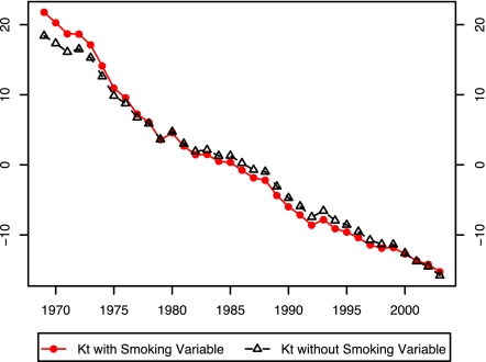
Fig. 5 shows the values of k_t produced by models with and without the smoking variable. Differences between the k_t series are not striking, but it should be recalled that in projections, k_t is multiplying the b_x, so that the same values of k_t may produce much different projections in the models with and without smoking variable.

Fig. 5.

Comparison of k_t values in models with and without smoking histories: United States, 1969–2003.

Projections.

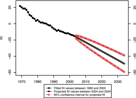
The first step in the projection process is forecasting the mortality index, k_t. We followed the standard procedures suggested by Box and Jenkins (18) and Makridakis et al. (19) to find the appropriate ARIMA time series model for the mortality trend, k_t. ARIMA (0, 1, 0)—in other words, random walk with drift—best describes our index. Using this model, we forecasted the values of k_t to year 2034. We ended the projection period in 2034 because that is the latest year for which we have actual data (in some cases, partial) on smoking behavior for all cohorts in the age range 50–84. Fig. 6 presents the fitted and projected values of k_t, with 95% confidence intervals for the projected values.

Fig. 6.

Fitted and projected k_t values: United States, 1969–2034.

To forecast age-specific mortality rates between 2004 and 2034 for the age interval 50–84, we also required smoking indices for all cohorts who will be alive during this period. Most of those cohorts were already beyond age 40, and their smoking behavior could simply be observed. For the 4 cohorts born 1965–1969, 1970–1974, 1975–1979, and 1980–1984, we must project some portion of their smoking histories.

Our estimation strategy was to predict the smoking index (cumulative years smoked by age 40) based on cumulative years smoked at successively earlier ages by using the experience of cohorts who have already reached age 40 years. In other words, we predicted the value of smoking by age 40 years based on regressions with independent variables representing cumulative smoking indexes by age 35, by age 30, by age 25, and by age 20 years. We also added a trend variable to the regressions. Regressions are estimated on data for the 16 cohorts for which we have complete data up to age 40 years. The regressions in all cases explain at least 97% of the variance in cumulative years of smoking before age 40 years. We used these models to estimate the smoking index required for the 4 cohorts who had not completed their pre-40 smoking histories (Fig. 2).^‡

Using the parameters from the fitted model and the projected k_t and smoking index, we produced the age-specific mortality rates for each age group 50–84 between 2004 and 2034. Fig. 7 presents the ratio of projected death rates in 2034 to those in 2003. The projected mortality declines are somewhat larger for males than for females, in part because larger declines in cohort smoking behavior are projected for males. It should be stressed that most of the changes in smoking behavior that are reflected in the projections are not speculative but have already been observed among cohorts before reaching age 40 years.

Fig. 7.

Ratio of projected age-specific mortality rate in 2034 to age-specific mortality rate in 2003 using a model with smoking histories.

To evaluate the effect on projections of adding the smoking variable, we also projected mortality for males and females from 2004 to 2034 using the Lee–Carter Model without the smoking variable. In Table 2, we summarize the impact of including smoking on the level of projected mortality in the form of the probability of surviving from age 50 to 85 years. Differences between the 2 projections are small in the early years and grow substantially over the projection period. For both sexes, faster declines in mortality are projected when smoking is accounted for than when it is not. The main reason for this outcome is that the prevalence of smoking has declined for cohorts that are about to enter the age categories under study.

Table 2.

Comparison of projection results using different models: United States 2004–2034

Year	Probability of surviving from age 50 to 85 years
	Lee–Carter model with smoking		Lee–Carter model without smoking
	Male	Female	Male	Female
2004	0.3186	0.4723	0.3130	0.4776
2009	0.3595	0.4976	0.3397	0.4970
2014	0.4038	0.5242	0.3664	0.5161
2019	0.4491	0.5512	0.3931	0.5348
2024	0.4929	0.5786	0.4196	0.5531
2029	0.5378	0.6066	0.4457	0.5710
2034	0.5775	0.6318	0.4714	0.5884

The projected declines in smoking are greatest for males at older ages. As can be inferred from Fig. 2, male smoking behavior before age 40 years was still near its peak in 2003 in the age interval 80–84. Because this age interval experienced rising or constant smoking levels throughout the period of observation, the observed mortality improvements in this age interval were relatively small. In the model without smoking histories, these small improvements are embodied in the relatively low b_x values at these ages, which produce relatively small mortality improvements during the projection period. In the model that includes smoking, the imminent declines in smoking behavior for cohorts entering these older ages result in much more rapid projected mortality improvement. Fig. 8 presents the ratio of projected age-specific death rates in 2034 in models with and without the smoking variable. As anticipated, the biggest difference between the models occurs for older males.

Fig. 8.

Ratio of projected age-specific mortality rates in 2034 from a model with to one without smoking histories.

At younger ages, smoking was already declining during much of the period of observation. These declines are reflected in relatively high values of b_x at younger ages in the model that does not include smoking histories. Thus, including smoking in the model makes little difference for projections at younger ages; the empirical effect of declining smoking is already reflected in the parameters of the model without the smoking variable. In fact, projected male mortality at these ages is slightly higher in the model with smoking than in the model without, because smoking declines are projected to decelerate at younger ages.

According to Table 2, by the end of the projection period in 2034, the male probability of surviving from age 50 to age 85 years is 22.5% greater (0.5775/0.4714) when smoking is accounted for than when it is not. The female difference is 7.4% (0.6318/0.5884). Because smoking declines have been larger among males than among females, the sex difference in mortality is projected to narrow faster when smoking is accounted for than when it is not. This narrowing of sex differentials continues a pattern that has been observed for the past several decades.

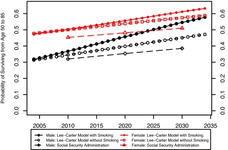
Both of the projections imply much faster improvements in mortality than those projected by the SSA (20). The SSA-projected male probability of surviving from age 50 to age 85 years in 2034 is only 0.397, compared with 0.578 in our smoking projection and 0.471 in our nonsmoking projection.^§ The SSA-projected female survival probability is 0.521, compared with 0.632 and 0.588 in our 2 projections. Fig. 9 presents the probability of surviving from age 50 to 85 years in the SSA projection and the 2 Lee–Carter projections. The SSA projections have often been criticized for projecting slow mortality improvements relative to Lee–Carter methods (11). If changes in smoking behavior are factored into the projections, the SSA projections appear even more conservative.

Fig. 9.

Probability of surviving from age 50 to 85 using different projection methods: United States, 2004–2034.

What may be bad news for the fiscal balance of the Social Security system is good news for the population as a whole and especially for men. Because of changes in smoking behavior that have already occurred or that can be reliably projected, American mortality is likely to fall more rapidly than is commonly anticipated.

References

- 1.Department of Health, Education, and Welfare. Smoking and Health: Report of the Advisory Committee to the Surgeon General of the Public Health Service. Washington, D.C: U.S. Department of Health, Education, and Welfare. Public Health Service; 1964. PHS Publ No 1103. [Google Scholar]
- 2.Preston S, Wang H. Sex mortality differences in the United States: The role of cohort smoking patterns. Demography. 2006;43:631–646. doi: 10.1353/dem.2006.0037. [DOI] [PubMed] [Google Scholar]
- 3.Burns D, et al. In: Changes in Cigarette-Related Disease Risk and Their Implicaitons for Prevention and Control. Burns D, Garfinkel L, Samet J, editors. Bethesda: Natl Inst Health; 1998. pp. 113–304. [Google Scholar]
- 4.Taylor D, Hasselblad V, Henley J, Thun M, Sloan F. Benefits of smoking cessation for longevity. Am J Public Health. 2002;92:990–996. doi: 10.2105/ajph.92.6.990. [DOI] [PMC free article] [PubMed] [Google Scholar]
- 5.Rogers R, Hummer R, Krueger P, Pampel F. Mortality attributable to cigarette smoking in the United States. Popul Dev Rev. 2005;31:259–292. doi: 10.1111/j.1728-4457.2005.00065.x. [DOI] [PMC free article] [PubMed] [Google Scholar]
- 6.Centers for Disease Control and Prevention. Morbidity and Mortality Weekly Report. Rockville, MD: DHHS; 1965–2004. Cigarette Smoking Among Adults–United States. [Google Scholar]
- 7.Burns D, et al. In: Smoking and Tobacco Control Monograph No. 8. Burns D, Garfinkel L, Samet J, editors. Bethesda: Natl Inst Health; 1998. pp. 13–112. [Google Scholar]
- 8.Gomez de Leon J, Texmon I. In: National Population Forecasting in Industrialized Countries. Keilman N, Cruijsen , editors. Amsterdam: Swets and Zeitlinger; 1992. pp. 61–74. [Google Scholar]
- 9.Lee R, Carter L. Modeling and forecasting U.S. Mortality. J Am Stat Assoc. 1992;87:659–671. [Google Scholar]
- 10.Hollman F, Mulder T, Kallan J. Methodology and Assumptions for the Population Projections of the United States 1999–2100. Washington: U.S. Census Bureau; 2000. Population Division Working Paper No 38. [Google Scholar]
- 11.Wilmoth J. Some methodological issues in mortality projection, based on an analysis of the U.S. Social Security system. Genus. 2005;XLI:179–211. [Google Scholar]
- 12.Lee R. The Lee-Carter Model for forecasting mortality, with various extensions and applications. North Am Actuar J. 2000;4:80–91. [Google Scholar]
- 13.Mokdad A, Marks J, Stroup D, Gerberding J. Actual causes of death in the United States, 2000. J Am Med Assoc. 2004;291:1238–1245. doi: 10.1001/jama.291.10.1238. [DOI] [PubMed] [Google Scholar]
- 14.Pampel F. Forecasting sex differences in mortality in high income nations: The contribution of smoking. Demogr Res. 2005;13:455–484. doi: 10.4054/DemRes.2005.13.18. [DOI] [PMC free article] [PubMed] [Google Scholar]
- 15.Bongaarts J. How long will we live? Pop Dev Rev. 2006;32:605–628. [Google Scholar]
- 16.van Hoorn W, De Beer J. In: Forecasting Mortality in Developed Countries: Insights from a Statistical, Demographic and Epidemiological Perspective. Tabeau E, van den Berg Jeths A, Heathcote C, editors. Dordrecht: Kluwer Academic; 2001. pp. 205–226. [Google Scholar]
- 17.Knoke J, et al. Lung cancer mortality is related to age in addition to duration and intensity of cigarette smoking: An analysis of CPS-I data. Cancer Epidemiol Biomark Prev. 2004;13:949–957. [PubMed] [Google Scholar]
- 18.Box G, Jenkins G. Time Series Analysis: Forecasting and Control. San Francisco: Holden-Day; 1970. [Google Scholar]
- 19.Makridakis S, Wheelwright S, Hyndman R. Forecasting: Methods and Applications. New York: John Wiley and Sons; 1998. [Google Scholar]
- 20.Bell F, Miller M. Life Tables for the United States Social Security Area 1900–2100. Baltimore, MD: Social Security Administration; 2006. Actuarial Study No. 116. [Google Scholar]