Multiresolution Bilateral Filtering for Image Denoising

Abstract

The bilateral filter is a nonlinear filter that does spatial averaging without smoothing edges; it has shown to be an effective image denoising technique. An important issue with the application of the bilateral filter is the selection of the filter parameters, which affect the results significantly. There are two main contributions of this paper. The first contribution is an empirical study of the optimal bilateral filter parameter selection in image denoising applications. The second contribution is an extension of the bilateral filter: multiresolution bilateral filter, where bilateral filtering is applied to the approximation (low-frequency) subbands of a signal decomposed using a wavelet filter bank. The multiresolution bilateral filter is combined with wavelet thresholding to form a new image denoising framework, which turns out to be very effective in eliminating noise in real noisy images. Experimental results with both simulated and real data are provided.

I. Introduction

There are different sources of noise in a digital image. Some noise components, such as the dark signal nonuniformity (DSNU) and the photoresponse nonuniformity (PRNU), display nonuniform spatial characteristics. This type of noise is often referred as fixed pattern noise (FPN) because the underlying spatial pattern is not time varying. Temporal noise, on the other hand, does not have a fixed spatial pattern. Dark current and photon shot noise, read noise, and reset noise are examples of temporal noise. The overall noise characteristics in an image depend on many factors, including sensor type, pixel dimensions, temperature, exposure time, and ISO speed. Noise is in general space varying and channel dependent. Blue channel is typically the noisiest channel due to the low transmittance of blue filters. In single-chip digital cameras, demosaicking algorithms are used to interpolate missing color components; hence, noise is not necessarily uncorrelated for different pixels. An often neglected characteristic of image noise is the spatial frequency. Referring to Figure 1, noise may have low-frequency (coarse-grain) and high-frequency (fine-grain) fluctuations. High-frequency noise is relatively easier to remove; on the other hand, it is difficult to distinguish between real signal and low-frequency noise.

Fig. 1.

Portion of an image captured with a Sony DCR-TRV27, and its red, green, and blue channels are shown in raster scan order. The blue channel is the most degraded channel; it has a coarse-grain noise characteristics. The red and green channels have finer-grain noise characteristics.

Many denoising methods have been developed over the years; among these methods, wavelet thresholding is one of the most popular approaches. In wavelet thresholding, a signal is decomposed into its approximation (low-frequency) and detail (high-frequency) subbands; since most of the image information is concentrated in a few large coefficients, the detail subbands are processed with hard or soft thresholding operations. The critical task in wavelet thresholding is the threshold selection. Various threshold selection strategies have been proposed, for example, VisuShrink [1], SureShrink [2], and BayesShrink [3]. In the VisuShrink approach, a universal threshold that is a function of the noise variance and the number of samples is developed based on the minimax error measure. The threshold value in the SureShrink approach is optimal in terms of the Stein’s unbiased risk estimator. The BayesShrink approach determines the threshold value in a Bayesian framework, through modeling the distribution of the wavelet coefficients as Gaussian. These shrinkage methods have later been improved by considering inter-scale and intra-scale correlations of the wavelet coefficients [4], [5], [6], [7], [8]. The method in [4] models the neighborhoods of coefficients at adjacent positions and scales as Gaussian scale mixture and applies the Bayesian least squares estimation technique to update the wavelet coefficients. The method, known as the BLS-GSM method, is one of the benchmarks in the denoising literature due to its outstanding PSNR performance. Some recent methods have surpassed the PSNR performance of [4]. Among these methods, [9] constructs a global field of Gaussian scale mixtures to model subbands of wavelet coefficients as a product of two independent homogeneous Gaussian Markov random fields, and develops an iterative denoising algorithm. [10], [11], [12] develop gray-scale and color image denoising algorithms based on sparse and redundant representations over learned dictionaries, where training and denoising use the K-SVD algorithm. [13], [14] group 2D image fragments into 3D data arrays, and apply a collaborative filtering procedure, which consists of 3D transformation, shrinkage of the transform spectrum, and inverse 3D transformation. [15] models an ideal image patch as a linear combination of noisy image patches and formulates a total least squares estimation algorithm.

A recently popular denosing method is the bilateral filter [16]. While the term “bilateral filter” was coined in [16], variants of it have been published as the sigma filter [17], the neighborhood filter [18], and the SUSAN filter [19]. The bilateral filter takes a weighted sum of the pixels in a local neighborhood; the weights depend on both the spatial distance and the intensity distance. In this way, edges are preserved well while noise is averaged out. Mathematically, at a pixel location x, the output of the bilateral filter is calculated as follows:

$$\stackrel{\sim }{I}(\mathbf{x})=\frac{1}{C}\sum _{\mathbf{y}\in \mathcal{N}(\mathbf{x})}{e}^{\frac{-{\Vert \mathbf{y}-\mathbf{x}\Vert }^2}{2{\sigma }_d^2}}{e}^{\frac{-\mid I(\mathbf{y})-I(\mathbf{x}){\mid }^2}{2{\sigma }_r^2}}I(\mathbf{y}),$$ (1)

where σ_d and σ_r are parameters controlling the fall-off of the weights in spatial and intensity domains, respectively, (x) is a spatial neighborhood of x, and C is the normalization constant:

$$C=\sum _{\mathbf{y}\in \mathcal{N}(\mathbf{x})}{e}^{\frac{-{\Vert \mathbf{y}-\mathbf{x}\Vert }^2}{2{\sigma }_d^2}}{e}^{\frac{-\mid I(\mathbf{y})-I(\mathbf{x}){\mid }^2}{2{\sigma }_r^2}}.$$ (2)

Although the bilateral filter was first proposed as an intuitive tool, recent papers have pointed out the connections with some well established techniques. In [20], it is shown that the bilateral filter is identical to the first iteration of the Jacobi algorithm (diagonal normalized steepest descent) with a specific cost function. [21] and [22] relate the bilateral filter with the anisotropic diffusion. The bilateral filter can also be viewed as an Euclidean approximation of the Beltrami flow, which produces a spectrum of image enhancement algorithms ranging from the L₂ linear diffusion to the L₁ nonlinear flows [23], [24], [25]. In [22], Buades et al. proposes a nonlocal means filter, where similarity of local patches is used in determining the pixel weights. When the patch size is reduced to one pixel, the nonlocal means filter becomes equivalent to the bilateral filter. [26] extends the work of [22] by controlling the neighborhood of each pixel adaptively.

In addition to image denoising, the bilateral filter has also been used in some other applications, including tone mapping [27], image enhancement [28], volumetric denoising [29], exposure correction [30], shape and detail enhancement from multiple images [31], and retinex [32]. [27] describes a fast implementation of the bilateral filter; the implementation is based on a piecewise-linear approximation in the intensity domain and appropriate sub-sampling in the spatial domain. [33] later derives an improved acceleration scheme for the filter through expressing it in a higher-dimensional space where the signal intensity is added as the third dimension to the spatial domain.

Although the bilateral filter is being used more and more widely, there is not much theoretical basis on selecting the optimal σ_d and σ_r values. These parameters are typically selected by trial and error. In Section II, we empirically analyze these parameters as a function of noise variance for image denoising applications. We will show that the value of σ_r is more critical than the value of σ_d; we will in fact show that the optimal value of σ_r (in the mean square error sense) is linearly proportional to the standard deviation of the noise. In Section III, we will propose an extension of the bilateral filter. We will argue that the image denoising performance of the bilateral filter can be improved by incorporating it into a multiresolution framework. This will be demonstrated in Section IV with simulations and real data experiments.

II. Parameter selection for the bilateral filter

There are two parameters that control the behavior of the bilateral filter. Referring to (1), σ_d and σ_r characterizes the spatial and intensity domain behaviors, respectively. In case of image denoising applications, the question of selecting optimal parameter values has not been answered completely from a theoretical perspective. [22] analyzes the behavior of the bilateral filter depending on the derivative of the input signal and σ_r/σ_d values. Conditions under which the filter behaves like a Gaussian filter, anisotropic filter, and shock filter were examined. [26] proposes an adaptive neighborhood size selection method for the non-local means algorithm, which can be considered as a generalization of the bilateral filter. The neighborhood size is chosen to minimize the upper bound of the local L₂ risk; however, the effect of the intensity domain parameter is not considered. In this section, we provide an empirical study of optimal parameter values as a function of noise variance, and we will see that the intensity domain parameter σ_r is more critical than the spatial domain parameter σ_d.

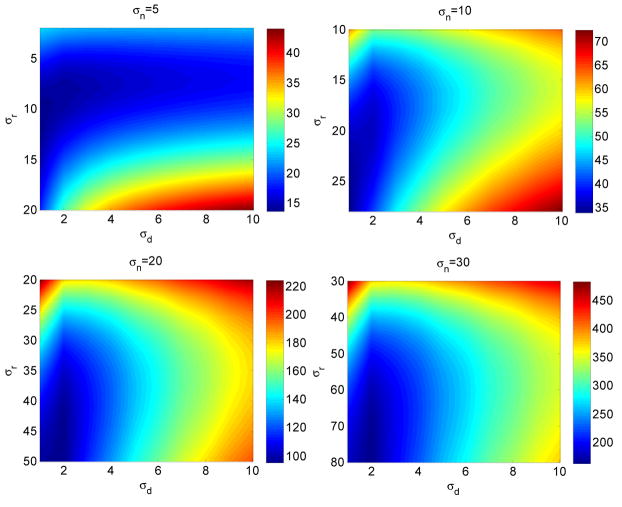
To understand the relationship among σ_d, σ_r, and the noise standard deviation σ_n, the following experiments were done. Zero-mean white Gaussian noise was added to some test images and the bilateral filter was applied for different values of the parameters σ_d and σ_r. The experiment was repeated for different noise variances and the mean squared error (MSE) values were recorded. The average MSE values are given in Figure 2. Examining these plots, it can be seen that the optimal σ_d value is relatively insensitive to noise variance compared to the optimal σ_r value. It appears that a good range for the σ_d value is roughly [1.5 – 2.1]; on the other hand, the optimal σ_r value changes significantly as the noise standard deviation σ_n changes. This is an expected result because if σ_r is smaller than σ_n, noisy data could remain isolated and untouched as in the case of the salt-and-pepper noise problem of the bilateral filter [16]. When σ_r is sufficiently large, σ_d becomes important; apparently, increasing the value of σ_d too much results in over-smoothing and decrease of MSE.

Fig. 2.

The MSE values between the original image and the denoised image for different values of σ_d, σ_r, and the noise standard deviation σ_n are displayed. The results displayed are average results for 200 images. The number of samples along the σ_d (and σ_r) direction is 10; the results are interpolated to produce smoother plots.

To see the relationship between σ_n and the optimal σ_r, we set σ_d to some constant values, and determined the optimal σ_r values (minimizing MSE) as a function of σ_n. The experiments were again repeated for a set of images; the average values and the standard deviations are displayed in Figure 3. We can make several observations from these plots: (1) Optimal σ_r and σ_n are linearly related to a large degree. (2) The standard deviation from the mean increases for larger values of σ_n. (3) When σ_d value is increased, the linearity between the optimal σ_r and σ_n still holds, but with lower slope. Obviously, there is no single value for (σ_r/σ_n) that is optimal for all images and σ_d values; in fact, future research should look for spatially adaptive parameter selection to take local texture characteristics into account. On the other hand, these experiments at least tell us some guidelines in selecting these parameters.

Fig. 3.

The optimal σ_r values as a function of the noise standard deviation σ_n are plotted based on the experiments with 200 test images. The blue data points are the mean of optimal σ_r values that produce the smallest MSE for each σ_n value. The blue vertical lines denote the standard deviation of the optimal σ_r for the test images. The least squares fits to the means of the optimal σ_r/σ_n data are plotted as red lines. The slopes of these lines are, from left to right, 2.56, 2.16, and 1.97.

III. A multiresolution image denoising framework

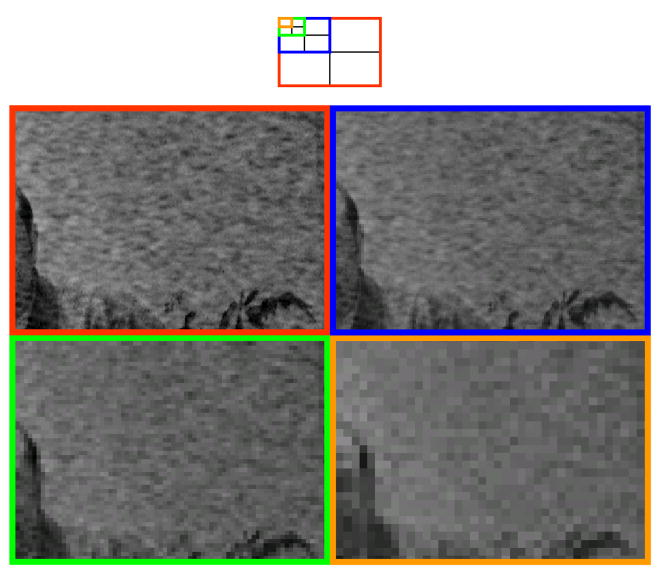
As we have discussed in Section I, image noise is not necessarily white and may have different spatial frequency (fine-grain and coarse-grain) characteristics. Multiresolution analysis has been proven to be an important tool for eliminating noise in signals; it is possible to distinguish between noise and image information better at one resolution level than another. Images in Figure 4 motivate the use of the bilateral filter in a multiresolution framework; in that figure, approximation subbands of a real noisy image are displayed. It is seen that the coarse-grain noise becomes fine-grain as the image is decomposed further into its subbands. While it is not possible to get rid of the coarse-grain noise at the highest level, it could be eliminated at a lower level.

Fig. 4.

Multiresolution characteristics of coarse-grain noise. A noisy image is decomposed into its frequency subbands using db8 filters of Matlab. Part of the image is shown at the original resolution level and at three approximation subbands. The coarse-grain noise at the original level is difficult to identify and eliminate; the noise becomes fine grain as the image is decomposed, and can be eliminated more easily.

The proposed framework is illustrated in Figure 5: A signal is decomposed into its frequency subbands with wavelet decomposition; as the signal is reconstructed back, bilateral filtering is applied to the approximation subbands. Unlike the standard single-level bilateral filter [16], this multiresolution bilateral filter has the potential of eliminating low-frequency noise components. (This will become evident in our experiments with real data. Such an observation was also made in [34] for anisotropic diffusion, which has been shown to be related to the bilateral filter. Also, [31] utilizes the bilateral filter (because it does not create halo artifacts) in a multiresolution scheme for shape and detail enhancement from multiple images.) Bilateral filtering works in approximation subbands; in addition, it is possible to apply wavelet thresholding to the detail subbands, where some noise components can be identified and removed effectively. This new image denoising framework combines bilateral filtering and wavelet thresholding. In the next section, we will demonstrate that this framework produces results better than the individual applications of the wavelet thresholding or the bilateral filter, or successive application of the wavelet thresholding and the bilateral filter. We will also discuss the contribution of the wavelet thresholding to overall performance.

Fig. 5.

Illustration of the proposed method. An input image is decomposed into its approximation and detail subbands through wavelet decomposition. As the image is reconstructed back, bilateral filtering is applied to the approximation subbands, and wavelet thresholding is applied to the detail subbands. The analysis and synthesis filters (L_a, H_a, L_s, and H_s) form a perfect reconstruction filter bank. The illustration shows one approximation subband and one detail subband at each decomposition level; this would be the case when the data is one dimensional. For a two-dimensional data, there are in fact one approximation and three (horizontal, vertical, and diagonal) detail subbands at each decomposition level. Also, in the illustration, there are two levels of decomposition; the approximation subbands could be decomposed further in an application.

IV. Experiments and Discussions

We have conducted some experiments to see the performance of the proposed framework quantitatively and visually. To do a quantitative comparison, we simulated noisy images by adding white Gaussian noise with various standard deviations to some standard test images. These noisy images were then denoised using several algorithms and the PSNR results were calculated. For visual comparisons, real noisy images were used.

A. PSNR Comparison for Simulated Noisy Images

For each test image, three noisy versions were created by adding white Gaussian noise with standard deviations 10, 20, and 30. PSNR results for six methods are included in Table I. The first method is the BayesShrink wavelet thresholding algorithm [3]. Five decomposition levels were used; the noise variance was estimated using the robust median estimator [1]. The second method is the bilateral filter [16]. Based on our experiments discussed in the previous sections, we chose the following parameters for the bilateral filter: σ_d = 1.8, σ_r = 2 × σ_n, and the window size is 11 × 11. The third method is the sequential application of [3] and [16]. The reason this method was included is to see the combined effect of [3] and [16] and compare it with the proposed method. The fourth method is the new SURE method of [8]. It was recently published, and shown to produce very good results with non-redundant wavelet decomposition. The fifth method is the 3D collaborative filtering (3DCF) of [13], [14]. The sixth method is the proposed method. For the proposed method, db8 filters in Matlab were used for one-level decomposition. For the bilateral filtering part of the proposed method, we set the parameters as follows: σ_d = 1.8, the window size is 11 × 11, and σ_r = 1.0 × σ_n at each level. (In case of the original bilateral filter, σ_r = 2 × σ_n was a better choice. However, for the proposed method this lead to a smaller PSNR value on average. The reason is the double application of the bilateral filter in the proposed method. When σ_r was large, the images were smoothed to produce low PSNR values. After some experimentation, σ_r = 1.0 × σ_n turned out to be a better choice in terms of PSNR values. Here, we should note that a higher PSNR does not necessarily correspond to a better visual quality. We will discuss this shortly.) For the wavelet thresholding part of the proposed method, the BayesShrink method [3] was used; and the noise variance was estimated again with the robust median estimator technique. To eliminate the border effects, images were mirror-extended before the application of the bilateral filter and cropped to the original size at the end.

TABLE I.

PSNR comparison of the BayesShrink method [3], the bilateral filter [16], sequential application of the BayesShrink [3] and the bilateral filter [16] methods, New SURE thresholding [8], 3DCF [14] and the proposed method for simulated additive white Gaussian noise of various standard deviations. (The numbers were obtained by averaging the results of six runs.)

Input Image	σn	BayesShrink [3]	Bilateral Filter [16]	[3] Followed by [16]	New SURE [8]	3DCF [14]	Proposed Method
Barbara 512 × 512	10	31.25	31.37	30.92	32.18	34.98	31.79
	20	27.32	27.02	27.16	27.98	31.78	27.74
	30	25.34	24.69	25.23	25.83	29.81	25.61
Boats 512 × 512	10	31.98	32.02	31.81	32.90	33.92	32.58
	20	28.55	28.40	28.43	29.47	30.88	29.25
	30	26.71	26.57	26.66	27.63	29.12	27.24
Goldhill 512 × 512	10	31.94	32.08	31.93	32.69	33.62	32.48
	20	28.69	28.90	28.80	29.52	30.72	29.50
	30	27.13	27.50	27.34	27.89	29.16	27.77
Peppers 256 × 256	10	31.49	32.98	31.89	33.18	34.68	33.45
	20	27.85	29.07	28.01	29.33	31.29	30.20
	30	25.73	27.02	26.07	27.13	29.28	28.18
House 256 × 256	10	33.07	33.77	33.09	34.29	36.71	34.62
	20	29.83	29.63	29.79	30.93	33.77	31.37
	30	27.12	28.11	28.10	28.98	32.09	29.24
Lena 512 × 512	10	33.38	33.65	33.39	34.45	35.93	34.48
	20	30.27	30.33	30.29	31.33	33.05	31.28
	30	28.60	28.54	28.62	29.55	31.26	29.33
Average		29.24	29.54	29.31	30.29	32.34	30.34

As seen in the PSNR results of Table I, the proposed method is 0.8dB better than the original bilateral filter and 1.1dB better than the BayesShrink method on average. The sequential application of [3] and [16] is only slightly better than [3] and worse than [16]. Therefore, we conclude that the improvement of the proposed method is not due to the combined effect of [3] and [16], but due to the multiresolution application of the bilateral filter. While the new SURE method [8] is slightly worse than the proposed method, the 3DCF method [14] is 2dB better than the proposed method.

Most of the denoising methods are optimized for additive white Gaussian noise (AWGN); however, the real challenge is the performance for real noisy images. While we cannot quantitatively evaluate the performances for real noisy images, we may simulate spatially varying noise and make a quantitative comparison for it. This is more challenging than the AWGN case and could be a better representative of the performance for nonuniform noise situations. In our experiments, the space varying noise is generated by using a two-dimensional sinusoid of the same size as the input image; and the standard deviation of the noise at each pixel is controlled based on the amplitude of the sinusoid. To be specific, we generated the 2D signal f(x_1, x₂) = (sin(x₁/T)sin(x₂/T) + 1)/2, where T is the period of the sinusoid. For an input image I(x₁, x₂), the noisy image is I(x_1, x₂)+ σ_d f(x_1, x₂). The experiment was repeated for several standard test images (for T = 10 and σ_d = 15); the results are shown in Table II. Notice that methods specifically designed for additive white Gaussian noise do not perform well for this experiment. The neighborhood based denoising method of [14], which can be considered as an extension of the bilateral filter, is still the best; however, compared to the simulated AWGN noise experiments, the gap between the proposed method and [14] is much smaller. The standard bilateral filter also produces very good results. This experiment tells the effectiveness of the neighborhood based approach in case of space varying noise.

TABLE II.

PSNR comparison of the BayesShrink method [3], the bilateral filter [16], 3DCF [14], New SURE thresholding [8], BLS-GSM [4], and the proposed method for the space varying noise simulation.

Input Image	BayesShrink [3]	Bilateral Filter [16]	3DCF [14]	New SURE [8]	BLS-GSM [4]	Proposed Method
Barbara 512 × 512	31.9	32.2	34.3	24.0	29.7	32.6
Lena 512 × 512	33.1	33.4	35.2	22.7	31.2	34.1
Goldhill 512 × 512	32.2	32.6	32.3	23.6	29.9	32.8
Boat 512 × 512	32.5	32.6	32.9	23.6	30.3	32.9
House 256 × 256	32.5	33.4	35.8	22.7	31.4	34.1
Peppers 256 × 256	31.8	33.4	33.8	23.4	31.3	33.7
Average	32.3	32.9	34.0	23.3	30.6	33.4

B. Visual Comparison for Real Noisy Images

PSNR comparisons with simulated white Gaussian noise tell only a part of the story: First, it is well known that the PSNR is not a very good measure of visual quality; second, the white Gaussian noise assumption is not always accurate for real images. As a result, experiments with real data and visual inspections are necessary to evaluate the real performance of image denoising algorithms.

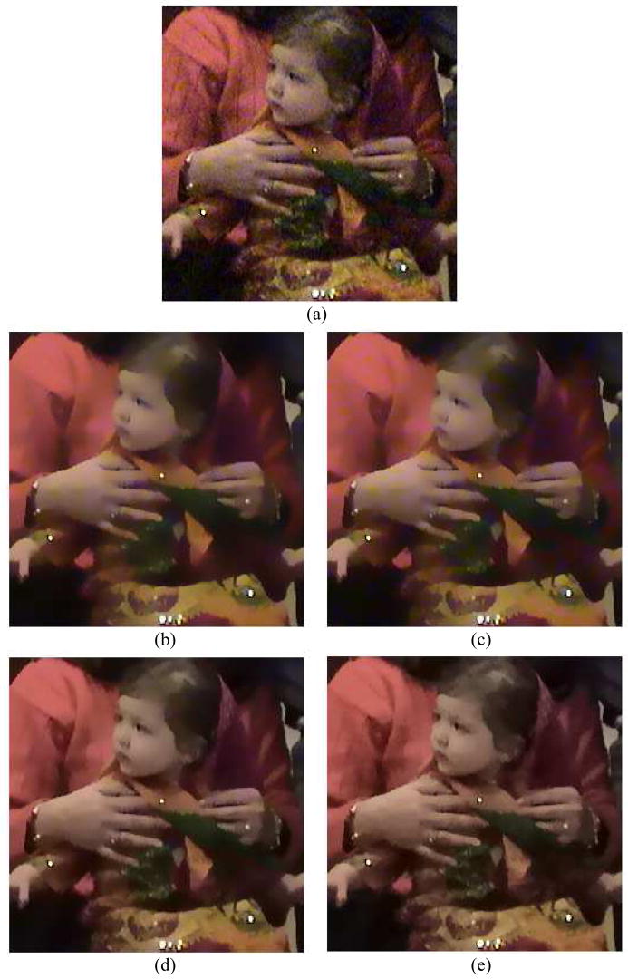
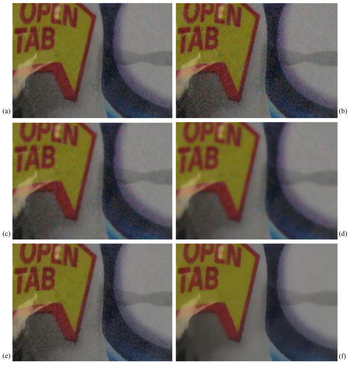
In case of color images, there is also the issue of what color space to use. To achieve good PSNR performance, the RGB space could be a good choice; however, for visual performance, it is a better idea to perform denoising in the perceptually uniform CIE-L^*a^*b^* color space. As humans find color noise more objectionable than luminance noise, stronger noise filtering could be applied to the color channels a^* and b^* compared to the luminance channel L^* without making the image visually blurry. Figure 6 provides results of the proposed method for the RGB and the L^*a^*b^* spaces. For the RGB space result (Figure 6(b)), the Euclidean distance between the (R,G,B) vectors is used as the intensity domain distance measure, and two levels of decomposition is applied to each channel. A close examination reveals that coarse-grain color artifacts are visible especially on the facial and hand regions. Figure 6(c) is the result when the Euclidean distance between the (L^*,a^*,b^*) vectors is used, and again two levels of decomposition is applied to each channel. The results in figures 6(b) and 6(c) are very similar. Figure 6(d) is the result when each channel is treated separately, and when the number of decomposition levels is 1,3, and 3 for L^*, a^*, and b^* channels, respectively. Figure 6(e) is the result when the Euclidean distance between the (L^*,a^*,b^*) vectors is used, and when the number of decomposition levels is 1,3, and 3 for L^*, a^*, and b^* channels, respectively. Notice that in Figures 6(d) and (e), texture is better preserved and coarse-grain noise is better eliminated compared to the previous results. Among the last two, there is not much observable difference. As a result, for perceptual reasons, we advocate applying and optimizing the denoising algorithms in the L^*a^*b^* space.

Fig. 6.

Comparison of the proposed method for different intensity distance measures and the number of decomposition levels. (a) Input image. (b) The distance measure is the Euclidean distance between (R,G,B) vectors. The number of decomposition levels is 2 for all channels. (c) The distance measure is the Euclidean distance between (L^*a^*b^*) vectors. The number of decomposition levels is 2 for all channels. (d) Each channel is denoised separately in L^*a^*b^* space. The number of decomposition levels is 1 for the L channel and 3 for the a^* and b^* channels. (e) The distance measure is the Euclidean distance between (L^*a^*b^*) vectors. The number of decomposition levels is 1 for the L channel and 3 for the a^* and b^* channels. (In these experiments, σ_d = 3, σ_r = 3 × σ_n, and σ_n is estimated using the robust median estimator [3].

Next, we show a set of results for real noisy images. In all these experiments, σ_d and σ_r parameters fixed at σ_d = 1.8 and σ_r = 3 × σ_n produced very good results for the proposed method. (σ_n was estimated using the robust median estimator [3] for all images.) Therefore, we can claim that the proposed method is data-driven and robust for good visual performance.

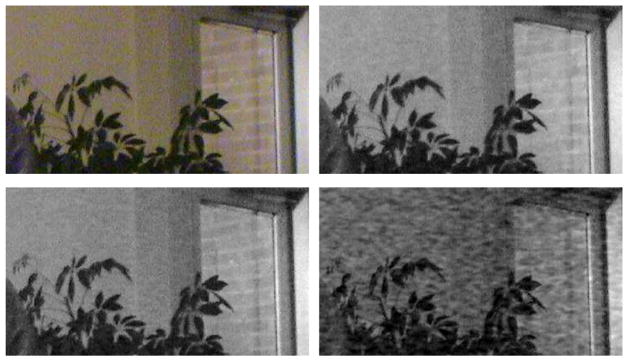
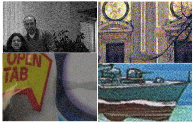
Figure 7 shows four test images. The first image is the blue channel of an image captured with Sony DCR-TRV27. The second image was captured with a Canon A530 at ISO 800. The other images were downloaded from [35].

Fig. 7.

Input images to be denoised using various algorithms. The top-left image is the blue channel of an image captured with Sony DCR-TRV27. The bottom-left image was captured with a Canon A530 at ISO 800. The other images were downloaded from [35].

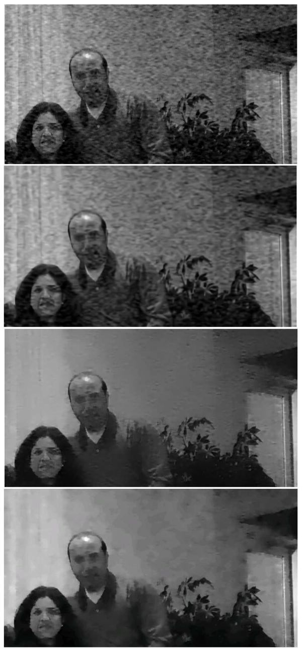
In Figure 8, we compare the standard bilateral filter, the 3DCF method [14], and the proposed method. The input image was corrupted significantly with coarse-grain noise. The results show that the standard bilateral filter and the 3DCF method are not effective against the coarse-grain noise. We provide two results for the proposed method. σ_r = 2 × σ_n for one result; and σ_r = 3 × σ_n for the other. The coarse grain noise is reduced significantly in both cases. While more noise components are eliminated for larger σ_r, contouring artifacts may start to appear, which is a common problem of the bilateral filtering and anisotropic diffusion.

Fig. 8.

From top to bottom: Result of (a) the bilateral filter [16] with σ_d =1.8 and σ_r = 2 × σ_n, (b) the 3DCF method [14], (c) the proposed method with the number of decomposition levels is 4, σ_d = 1.8, and σ_r = 2 × σ_n at each level, (d) the proposed method with the number of decomposition levels is 4, σ_d = 1.8, and σ_r = 3 × σ_n at each level. The subband decomposition filters are db8 in Matlab.

In Figure 9, we compare the 3DCF method [14], the standard bilateral filter and the proposed method. The standard bilateral filter was tested for various values of σ_d and σ_r. Some representative results are shown. As seen in figures 9(b–d), no matter what parameter values are chosen for the standard bilateral filter, the coarse-grain chroma noise could not be eliminated effectively. (We have also tested the iterative application of the bilateral filter. The results were not good either, and were not included in the figure.) Two results obtained by the proposed method are given: For the result in Figure 9(e), the number of decomposition levels for the luminance channel is one; and in Figure 9(f) it is two. For both results, the number of decomposition levels for the chrominance channels is four. Coarse-grain chroma noise is eliminated in both cases. Increasing the number of decomposition levels for the luminance channel produces a smoother image as seen in Figure 9(f).

Fig. 9.

(a) Result of the 3DCF method [14], (b) The bilateral filter [16] with σ_d = 1.8 and σ_r = 3 × σ_n, (c) The bilateral filter [16] with σ_d = 1.8 and σ_r = 20 × σ_n, (d) The bilateral filter [16] with σ_d = 5.0 and σ_r = 20 × σ_n, (e) The proposed method with the number of decomposition levels is (1, 4, 4) for the (L_*, a_*, b_*) channels, respectively. That is, the L_* channel is decomposed one level, and a_* and b_* channels are decomposed four levels. (f) The proposed method with the number of decomposition levels is (2, 4, 4) for the (L_*, a_*, b_*) channels, respectively. For the proposed method, σ_d = 1.8, and σ_r = 3 × σ_n at each level. The subband decomposition filters are db8 in Matlab. The noise parameter σ_n is estimated using the robust median estimator.

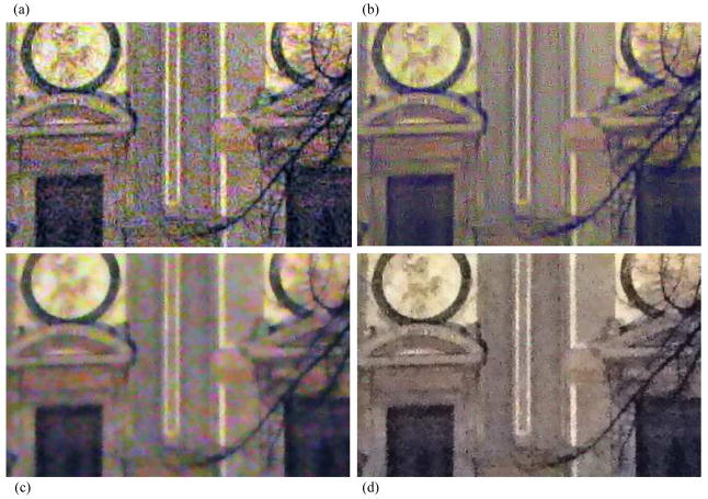
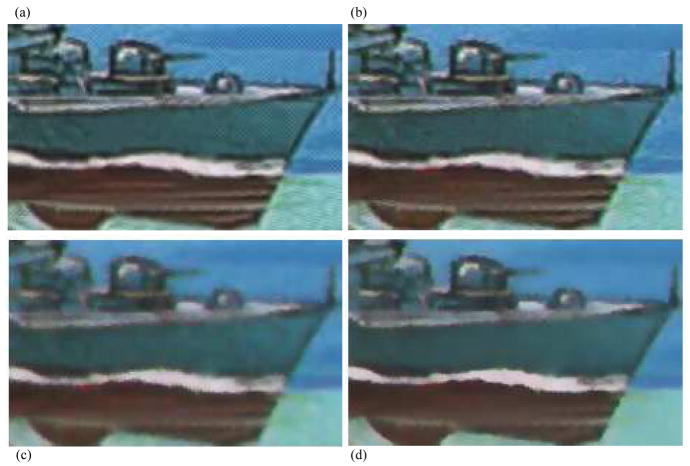
In Figures 10 and 11, results of the 3DCF method [14], the BLS-GSM method [4], the bilateral filter [16], and the proposed method are presented for real images provided at [35]. Among these methods, the proposed method is apparently producing more visually pleasing results than the others. Notice the lack of color in Figure 10 for the proposed method; this is due to the higher number of decomposition levels for the chrominance channels. If the number of decomposition levels is reduced, the result would be more colorful. In Figure 11, noise was not completely eliminated by the 3DCF or the BLS-GSM methods. The result of the bilateral filter is less noisy but overly smoothed. The result of the proposed method can be considered as the best visual one among three.

Fig. 10.

(a) Result of the 3DCF method [14], (b) The BLS-GSM result obtained from [35] (c) The bilateral filter [16] result, (d) Result of the proposed method. For the bilateral filter, σ_d = 1.8, σ_r = 10 × σ_n, and the window size is 11 × 11. For the proposed method, σ_d = 1.8, σ_r = 3 × σ_n at each level, the window size is 11 × 11, and the number of decomposition levels is (1, 4, 4) for the (L_*, a_*, b_*) channels, respectively. The wavelet filters are db8 in Matlab. The noise parameter σ_n is estimated using the robust median estimator.

Fig. 11.

(a) Result of the 3DCF method [14], (b) The BLS-GSM result obtained from [35] (c) The bilateral filter [16] result, (d) Result of the proposed method. For the bilateral filter, σ_d = 1.8, σ_r = 10 × σ_n, and the window size is 11 × 11. For the proposed method, σ_d = 1.8, σ_r = 3 × σ_n at each level, the window size is 11 × 11, and the number of decomposition levels is (1, 4, 4) for the (L_*, a_*, b_*) channels, respectively. The wavelet filters are db8 in Matlab. The noise parameter σ_n is estimated using the robust median estimator.

Finally, we should comment on the contribution of the wavelet thresholding to the multiresolution framework. (As mentioned earlier, in our experiments, we used the BayesShrink method [3] for the wavelet thresholding part.) We have done experiments with and without the wavelet thresholding. For real image experiments, the difference is barely visible. That is, the dominant contribution is coming from the multiresolution bilateral filtering, and the contribution of wavelet thresholding is little. On the other hand, in additive white Gaussian noise simulations, wavelet thresholding has resulted in an improvement of about 0.5dB in PSNR. Considering all aspects, we did not want to exclude wavelet thresholding from the proposed framework because another wavelet thresholding method could produce better results; and we leave the investigation of this as a future work.

V. Conclusions

In this paper we make an empirical study of the optimal parameter values for the bilateral filter in image denoising applications and present a multiresolution image denoising framework, which integrates bilateral filtering and wavelet thresholding. In this framework, we decompose an image into low- and high-frequency components, and apply bilateral filtering on the approximation subbands and wavelet thresholding on the detail subbands. We have found that the optimal σ_r value of the bilateral filter is linearly proportional to the standard deviation of the noise. The optimal value of the σ_d is relatively independent of the noise power. Based on these results, we estimate the noise standard deviation at each level of the subband decomposition and use a constant multiple of it for the σ_r value of bilateral filtering. The experiments with real data demonstrate the effectiveness of the proposed method.

Note that in all real image experiments, σ_n values were estimated from the data, and the same σ_d and (σ_r/σ_n) values produced satisfactorily good results for the proposed method. That is, once the parameters were decided, there was no need to re-adjust them for another image.

The key factor in the performance of the proposed method is the multiresolution application of the bilateral filter. It helped eliminating the coarse-grain noise in images. The wavelet thresholding adds power the proposed method as some noise components can be eliminated better in detail subbands. We used a specific wavelet thresholding technique (i.e., the BayesShrink method); it is possible to improve the results further by using better detail-subband-denoising techniques or using redundant wavelet decomposition. These issues and the detailed analysis of parameter selection for the proposed framework are left as future work. We believe that the proposed framework will inspire further research towards understanding and eliminating noise in real images and help better understanding of the bilateral filter.

References

- 1.Donoho DL, Johnstone IM. Ideal spatial adaptation by wavelet shrinkage. Biometrika. 81(3):425–455. 1994. [Google Scholar]
- 2.Donoho DL, Johnstone IM, Kerkyacharian G, Picard D. Wavelet shrinkage: Asymptopia? Journal of Royal Statistics Society, Series B. 57(2):301–369. 1995. [Google Scholar]
- 3.Chang SG, Yu B, Vetterli M. Adaptive wavelet thresholding for image denoising and compression. IEEE Trans Image Processing. 2000 September;9(9):1532–1546. doi: 10.1109/83.862633. [DOI] [PubMed] [Google Scholar]
- 4.Portilla J, Strela V, Wainwright MJ, Simoncelli EP. Image denoising using scale mixtures of gaussians in the wavelet domain. IEEE Trans Image Processing. 2003 November;12(11):1338–1351. doi: 10.1109/TIP.2003.818640. [DOI] [PubMed] [Google Scholar]
- 5.Pizurica A, Philips W. Estimating the probability of the presence of a signal of interest in multiresolution single- and multiband image denoising. IEEE Trans Image Processing. 2006 March;15(3):654–665. doi: 10.1109/tip.2005.863698. [DOI] [PubMed] [Google Scholar]
- 6.Sendur L, Selesnick IW. Bivariate shrinkage functions for wavelet-based denoising exploiting interscale dependency. IEEE Trans Signal Processing. 2002 November;50(11):2744–2756. [Google Scholar]
- 7.Sendur L, Selesnick IW. Bivariate shrinkage with local variance estimation. IEEE Signal Processing Letters. 2002 December;9(12):438–441. [Google Scholar]
- 8.Luisier F, Blu T, Unser M. A new sure approach to image denoising: Inter-scale orthonormal wavelet thresholding. IEEE Trans Image Processing. 2007 March;16(3):593–606. doi: 10.1109/tip.2007.891064. [DOI] [PubMed] [Google Scholar]
- 9.Lyu S, Simoncelli EP. Statistical modeling of images with fields of gaussian scale mixtures. In: Schölkopf B, Platt J, Hoffman T, editors. Advances in Neural Information Processing Systems. Vol. 19. MIT Press; Cambridge, MA: 2007. pp. 945–952. [Google Scholar]
- 10.Elad M, Aharon M. Image denoising via learned dictionaries and sparse representation. Proc. IEEE Computer Vision and Pattern Recognition; June 2006; [DOI] [PubMed] [Google Scholar]
- 11.Elad M, Aharon M. Image denoising via sparse and redundant representations over learned dictionaries. IEEE Trans Image Processing. 2006 December;15(12):3736–3745. doi: 10.1109/tip.2006.881969. [DOI] [PubMed] [Google Scholar]
- 12.Mairal J, Elad M, Sapiro G. Sparse representation for color image restoration. IEEE Trans Image Processing. 2008 January;17(1):53–69. doi: 10.1109/tip.2007.911828. [DOI] [PubMed] [Google Scholar]
- 13.Dabov K, Katkovnik V, Foi A, Egiazarian K. Image denoising with block-matching and 3d filtering. Proc. SPIE Electronic Imaging: Algorithms and Systems V; January 2006; [Google Scholar]
- 14.Dabov K, Foi A, Katkovnik V, Egiazarian K. Image denoising by sparse 3d transform-domain collaborative filtering. IEEE Trans Image Processing. 16:2080–2095. 2007. doi: 10.1109/tip.2007.901238. [DOI] [PubMed] [Google Scholar]
- 15.Hirakawa K, Parks TW. Image denoising using total least squares. IEEE Trans Image Processing. 2006 September;15(9):2730–2742. doi: 10.1109/tip.2006.877352. [DOI] [PubMed] [Google Scholar]
- 16.Tomasi C, Manduchi R. Bilateral filtering for gray and color images. Proc Int Conf Computer Vision. 1998:839–846. [Google Scholar]
- 17.Lee JS. Digital image smoothing and the sigma filter. CVGIP: Graphical Models and Image Processing. 1983 November;24(2):255–269. [Google Scholar]
- 18.Yaroslavsky L. Digital Picture Processing - An Introduction. Springer Verlag; 1985. [Google Scholar]
- 19.Smith SM, Brady JM. Susan - a new approach to low level image processing. Int Journal of Computer Vision. 1997;23:45–78. [Google Scholar]
- 20.Elad M. On the origin of the bilateral filter and ways to improve it. IEEE Trans Image Processing. 2002 October;11(10):1141–1151. doi: 10.1109/TIP.2002.801126. [DOI] [PubMed] [Google Scholar]
- 21.Barash D. A fundamental relationship between bilateral filtering, adaptive smoothing, and the nonlinear diffusion equation. IEEE Trans Pattern Analysis and Machine Intelligence. 2002 June;24(6):844–847. [Google Scholar]
- 22.Buades A, Coll B, Morel J. Neighborhood filters and pde’s. Numerische Mathematik. 105:1–34. 2006. [Google Scholar]
- 23.Sochen N, Kimmel R, Malladi R. A general framework for low level vision. IEEE Trans Image Processing. 1998 March;7(3):310–318. doi: 10.1109/83.661181. [DOI] [PubMed] [Google Scholar]
- 24.Sochen N, Kimmel R, Bruckstein AM. Diffusions and confusions in signal and image processing. Journal of Mathematical Imaging and Vision. 14(3):195–209. 2001. [Google Scholar]
- 25.Spira A, Kimmel R, Sochen N. A short time beltrami kernel for smoothing images and manifolds. IEEE Trans Image Processing. 2007 June;16(6):1628–1636. doi: 10.1109/tip.2007.894253. [DOI] [PubMed] [Google Scholar]
- 26.Kervrann C, Boulanger J. Optimal spatial adaptation for patch-based image denoising. IEEE Trans Image Processing. 2006 October;15(10):2866–2878. doi: 10.1109/tip.2006.877529. [DOI] [PubMed] [Google Scholar]
- 27.Durand F, Dorsey J. Fast bilateral filtering for the display of high-dynamic-range images. Proc SIGGRAPH. 2002:257–266. [Google Scholar]
- 28.Eisemann E, Durand F. Flash photography enhancement via intrinsic relighting. Proc SIGGRAPH. 2004:673–678. [Google Scholar]
- 29.Wong WCK, Chung ACS, Yu SCH. Trilateral filtering for biomedical images. Proc IEEE Int Symposium on Biomedical Imaging. 2004:820–823. [Google Scholar]
- 30.Bennett EP, McMillan L. Video enhancement using per-pixel virtual exposures. ACM Trans on Graphics. 24(3):845–852. 2005. [Google Scholar]
- 31.Fattal R, Agrawala M, Rusinkiewicz S. Multiscale shape and detail enhancement from multi-light image collections. ACM Transactions on Graphics (Proc SIGGRAPH) 2007 August;26(3) [Google Scholar]
- 32.Elad M. Scale-Space, Lecture-notes in Computer-Science. Apr, 2005. Retinex by two bilateral filters; pp. 7–10. [Google Scholar]
- 33.Paris S, Durand F. A fast approximation of the bilateral filter using a signal processing approach. Proc European Conference on Computer Vision. 2006:568–580. [Google Scholar]
- 34.Acton S. Multigrid anisotropic diffusion. IEEE Trans Image Processing. 1998 March;7(3):280–291. doi: 10.1109/83.661178. [DOI] [PubMed] [Google Scholar]
- 35.“Color test images,” [Available online: http://decsai.ugr.es/javier/denoise], April 2008.