Decision analysis for the evaluation of diagnostic tests, prediction models and molecular markers

Abstract

The traditional statistical approach to the evaluation of diagnostic tests, prediction models and molecular markers is to assess their accuracy, using metrics such as sensitivity, specificity and the receiver-operating-characteristic curve. However, there is no obvious association between accuracy and clinical value: it is unclear, for example, just how accurate a test needs to be in order for it to be considered "accurate enough" to warrant its use in patient care. Decision analysis aims to assess the clinical value of a test by assigning weights to each possible consequence. These methods have been historically considered unattractive to the practicing biostatistician because additional data from the literature, or subjective assessments from individual patients or clinicians, are needed in order to assign weights appropriately. Decision analytic methods are available that can reduce these additional requirements. These methods can provide insight into the consequences of using a test, model or marker in clinical practice.

Introduction

Much of clinical medicine concerns diagnosis and prediction: patients want to know what they have ("Do I have cancer?"), and what is likely to happen to them ("Will I be cured or will the cancer come back?"); clinicians want to know what to treat ("Should I operate?") and how aggressive treatment should be ("Should I also give chemotherapy?"). Diagnosis and prediction have traditionally been based on the clinical history and physical examination. Recent years has seen an upsurge of interest in molecular markers of disease, based on sophisticated analysis of blood or tissue, particularly with respect to genomic information. For example, predicting a breast cancer patient's risk of recurrence traditionally depended on determining how far the cancer had spread (cancer stage); it has recently been suggested that genetic mutations in breast cancer cells also predict disease behavior (Marchionni et al. 2008).

From a statistical standpoint, prediction and diagnosis present similar analytic challenges: in both cases our data set consists of an estimate on the basis of a test T (with values T⁺ and T⁻, for “positive” and “negative”), a true disease state D (with values D⁺ and D⁻, for “diseased” and “non-diseased”). The traditional statistical approach has been to assess accuracy, typically defined using a measure of association between T and D. However, accuracy metrics have questionable clinical relevance. As an alternative, decision analytic methods have been proposed that can evaluate diagnostic tests, predictive models or molecular markers in terms of their real clinical consequences. A drawback of such methods is the requirement of additional information about clinical benefits and harms. However, some novel statistical methods are available to reduce these additional requirements.

Statistical approaches to evaluation of tests, models and markers

Consider the diagnosis of prostate cancer using the molecular marker prostate-specific antigen (PSA). Men with elevated levels of PSA in the blood are typically referred for prostate biopsy. However, only a minority of men with high PSA, around 20 – 25%, actually have prostate cancer. Some researchers have suggested that the level of unbound PSA ("free" PSA) can distinguish prostate cancer from benign prostate disease; specifically, cancer is more likely if the ratio between total and free PSA is low (Roddam et al., 2005). To investigate the value of free-to-total PSA ratio, I will use a data set from the Gotebörg site of the European Randomized Study of Screening for Prostate Cancer (ERSPC) (Schroder et al. 2003). The data set consists of 753 Swedish men with elevated PSA (3 ng / ml or higher) who were biopsied, of whom 192 were found to have prostate cancer. The study question is whether free-to-total PSA ratio can help determine which men really have prostate cancer, and hence should undergo biopsy, and which men do not have cancer, and who should therefore avoid what would be an unnecessary biopsy.

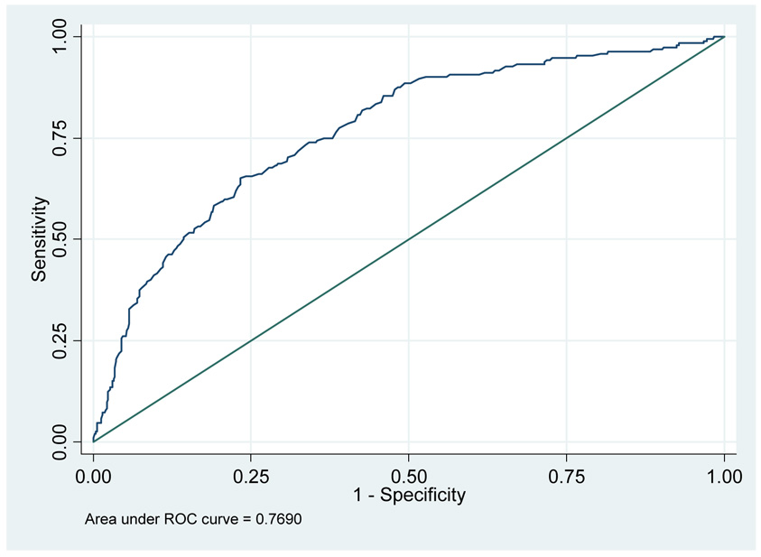
The simplest approach is to use free-to-total PSA ratio as a binary test: for example, men with a ratio of 0.18 or less are defined as positive (T⁺) and require biopsy, whereas those with free-to-total PSA ratio above 0.18 are defined as negative (T⁻) and do not need biopsy. Traditional biostatistical analysis starts by creating a two-by-two table of D by T and then calculates accuracy metrics such as sensitivity Sens = P(T⁺ | D⁺) and specificity Spec = P(T⁻ | D⁻). Table 1 gives sensitivity and specificity estimates, using the ERSPC data set, for various cut-points of free-to-total PSA ratio. If such calculations are repeated for the entire range of free-to-total PSA values, we can plot Sens versus 1 – Spec to obtain the receiver-operating-characteristic (ROC) curve, with the area-under-the-curve (AUC) providing a global metric of test accuracy. Figure 1 gives the ROC curve for free-to-total PSA ratio and positive biopsy in men with elevated PSA, with AUC=0.769.

Table 1.

Sensitivity and specificity for various cut-points of free-to-total PSA ratio for predicting prostate cancer in men with elevated PSA

Cut-point for free-to-total PSA ratio	Sensitivity	Specificity
0.18	88%	53%
0.15	71%	68%
0.20	91%	39%

Figure 1.

ROC curve for free-to-total PSA ratio in men with elevated PSA

Limitations of accuracy metrics

There are two general problems with accuracy metrics such as sensitivity, specificity and AUC. In general, an accurate test, model or marker is more likely to be useful than one less accurate, but it is difficult to know for any specific situation whether the accuracy of a test is high enough to warrant implementation in the clinic. Does an AUC of 0.769 mean that free-to-total PSA ratio should be used to determine who does or does not get biopsy, or would some higher value, say, 0.850, be required?

The second problem with accuracy metrics concerns the choice of cut-point. Assuming that we did decide to use free-to-total PSA ratio to determine which men with elevated PSA were referred to biopsy, what value should we use as the criterion for biopsy? In the case of cancer, sensitivity is valued over specificity, but it is difficult to say which combination of sensitivity and specificity in Table 1 is optimal.

Incorporating clinical consequences

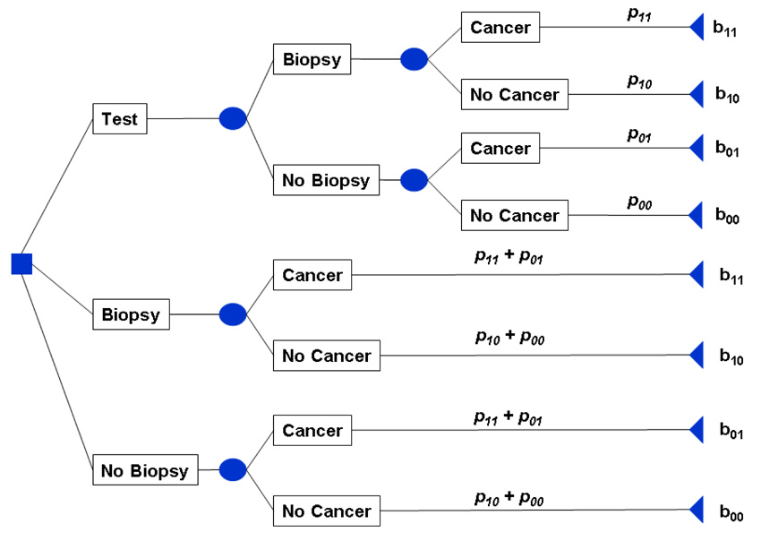
In decision analysis, one identifies possible actions and consequences, and selects the action with the best expected consequence. Often this process is aided by constructing a "decision tree," such as the shown in Figure 2 for prostate biopsy in men with elevated PSA. The principal of the decision tree is first to identify every possible decision, then identify every possible consequence of each decision, and finally to assign a probability and a benefit to each consequence (Hunink et al. 2001). We denote probabilities as p_xy and benefits as b_xy where x is an indicator for the test result and y is the indicator for disease.

Figure 2.

Decision tree for prostate cancer biopsy in men with elevated PSA

When faced with an elevated PSA, a patient has to decide among three options: undergo biopsy without further testing; refuse biopsy; undergo further testing and decide whether or not to have biopsy dependent on the results of those tests. A patient either has cancer or does not, and so the four possible consequences are finding cancer (true positive, p₁₁ and b₁₁); unnecessary biopsy (false positive, p₁₀ and b₁₀); missing cancer (false negative, p₀₁ and b₀₁); and avoiding unnecessary biopsy (true negative; p₀₀ and b₀₀). In the case of decisions for or against biopsy without further testing, the probability of each outcome depends on the prevalence π = P(D⁺) of prostate cancer. In the case of additional testing, these probabilities are also dependent on the sensitivity and specificity of the additional test as follows:

$$\begin{array}{c}{p}_{11}=\mathit{\text{Sens}}\times \pi \hfill \\ p_{10}=(1-\mathit{\text{Spec}})\times (1-\pi )\hfill \\ p_{01}=(1-\mathit{\text{Sens}})\times \pi \hfill \\ p_{00}=\mathit{\text{Spec}}\times (1-\pi )\hfill \end{array}$$

The values of each outcome b₁₁, b₁₀, b₀₁ and b₀₀ are difficult to specify. One approach is to use published estimates. For example, Berry and Parmigiani (1998) used published values related to quality of life in a decision analysis of breast cancer screening. The problem for the practicing biostatistician is that obtaining such values from the published literature can be time-consuming, that estimates can vary substantially between different papers and that converting published estimates (such as the probability of a localized cancer progressing in 10 years) into a benefit parameter on a 0 – 1 scale can be complex.

A simple alternative is to fix the best possible outcome at 1 (in this case, no biopsy and no disease, true negative, b₀₀ = 1) and the worst at 0 (no biopsy and disease, false negative, b₀₁= 0), hence only two remaining values need be specified. For now assume that, following a discussion with a clinician, we obtain, b₁₁ and b₁₀ of 0.6 and 0.85, respectively.

The optimal decision is the one with the highest expected benefit. Table 2 shows the results of the decision tree using a cut-point of 0.18 for free-to-total PSA ratio, where the prevalence of prostate cancer is π̂ =25%. The estimated expected benefit for using the free-to-total PSA ratio is 0.827, which is higher than the values for either biopsying everyone (0.786) or no-one (0.745). Therefore the strategy of undergoing further testing for all men with elevated PSA, and then sending for biopsy those with a ratio of 0.18 or less, is estimated to be optimal.

Table 2.

Use of a decision tree to make a biopsy decision

Parameters	Value		Expected outcome
			Strategy	Expected value	Expected value	Total
Health values for each outcome			Test	b11 × p11	0.6 × 22.44%	0.135
b11 (true positive, biopsy cancer)	0.6			b10 × p10	0.85 × 35.02%	0.298
b10 (false positive, unnecessary biopsy)	0.85			b01 × p01	0 × 3.06%	0.000
b01 (false negative, missed cancer)	0			b00 × p00	1 × 39.49%	0.395
b00 (true negative, avoid biopsy)	1					0.827
Prevalence (π)	25.5%
Sensitivity (Sens)	88%		Biopsy	b11 × (p11 + p01)	0.6 × 25.5%	0.153
Specificity (Spec)	53%			b10 × (p10 + p00)	0.85 × 74.5%	0.633
Probability of each outcome						0.786
p11: Sens × π	22.44%
p10: (1−Spec) × (1− π)	35.02%		No biopsy	b01 × (p11 + p01)	0 × 25.5%	0
p01: (1−Sens) × π	3.06%			b00 × (p10 + p00)	1 × 74.5%	0.75
p00: Spec × (1− π)	39.49%					0.75

Drawbacks of conventional decision analysis

Determining values for b₁₁, b₁₀ used in Table 2 involve judgments about the relative harm of a missed cancer versus an unnecessary biopsy. Patients' and physicians' judgments can vary on this point: for example, some patients do not tolerate invasive procedures such as biopsy particularly well. So while a standard decision analysis such as that in Table 2 may be a good starting point, in theory we should ask each physician or patient to evaluate benefits and harms individually, use their answers in the decision tree, and then work out whether outcome would be improved by using free-to-total PSA. This can be difficult to do, especially as the benefit parameters are not intuitive to specify.

From the analyst’s point of view, the determination of b₁₁, b₁₀, whether from the literature or from individual patients or physicians, is problematic. In the next section, I show how an alternative parameter, the threshold probability, can be used in decision analysis.

Using threshold probability in decision analysis

Suppose it is possible to specify a p_t, the threshold probability of disease for taking some action, such as biopsying a man for prostate cancer: if a patient's estimated probability of disease is greater than p_t he will opt for biopsy; if it is less than p_t, he will not opt for biopsy. By definition, when the probability of disease is equal to the threshold probability p_t, the benefits of opting for biopsy or no biopsy are equal. Thus:

$$b_{11}\times p_t+b_{10}\times (1-p_t)=b_{01}\times p_t+b_{00}\times (1-p_t)$$

And therefore

$$(b_{00}-b_{10})/(b_{11}-b_{01})=p_t/(1-p_t)$$ (1)

Now b₀₀ – b₁₀ is the benefit of true negative result compared to a false positive result; in clinical terms, the benefit of avoiding unnecessary treatment such as a negative biopsy. Comparably, b₁₁ – b₀₁ is the benefit of a true positive result compared to a false negative result; in other words, the benefit of treatment where it is indicated. Equation (1) therefore tells us that the threshold probability at which a patient will opt for treatment is informative of how a patient weighs the relative benefit of appropriate treatment compared to the benefit of avoiding unnecessary treatment (Pauker and Kassirer 1980).

We can rearrange (1) to obtain:

$$-(b_{10}-b_{00})=(b_{11}-b_{01})\times p_t/(1-p_t)$$ (2)

This states that the harm of a false positive compared to a true negative, is equal to the benefit of a true positive compared to a false negative, multiplied by the odds at p_t. A “net benefit” is benefit minus harm, thus the theoretical relationship in (2) allows us to define a net benefit (first described by CS Peirce (Baker and Kramer 2007)):

$$\frac{\mathit{\text{True Positive Count}}-\mathit{\text{False Positive Count}}\times \left(\frac{p_t}{1-p_t}\right)}{\mathit{\text{Total Sample Size}}}$$ (3)

This expression is equivalent to:

$$\mathit{\text{Sens}}\times \pi -(1-\text{Spec})\times (1-\pi )\times \left(\frac{p_t}{1-p_t}\right)$$ (4)

There are three advantages to using the threshold probability p_t in place of the benefit parameters b_xy. First, only a single parameter needs to be chosen. Second, the units of the parameter are more intuitive: patients and clinicians understand the concept of risk much more easily than the idea of a health state value on a scale of 0 to 1. Indeed, threshold probability is closely related to a widely-used statistic, positive predictive value. For example, it has been argued that the positive predictive value of a screening test for ovarian cancer needs to be at least 10%, because clinicians would be unwilling to conduct more than 10 surgeries to find a single case of ovarian cancer(Skates et al., 1995). Accordingly, we might therefore use a p_t of 10% in a decision analysis of ovarian cancer. Third, a threshold probability can be used both for weighting true and false positive test results and for determining the cut-off for a positive test result: instead of arbitrarily choosing a free-to-total PSA ratio cut-off of 0.18, 0.15 or 0.20, we calculate probabilities of cancer by logistic regression and use the threshold probability as the cut-off.

Following Vergouwe et al. (2002), a straightforward decision analytic method for determining the value of a diagnostic test, predictive model or molecular marker is as follows:

1. Obtain a threshold probability (p_t) for treatment

2. If necessary, use logistic regression to convert the results of the test, marker or model into a predicted probability of disease p̑

3. Define patients as test positive if p̑ ≥ p_t and negative otherwise. For a binary diagnostic test, p̂ is 1 for positive and 0 for negative

4. Calculate net benefit of the test, marker or model using the formula for net benefit in equation (3) or (4)

5. Calculate clinical net benefit for the strategy of treating all patients. As sensitivity is 100% and specificity 0%, (4) simplifies to:

   $$\pi -(1-\pi )\times \left(\frac{p_t}{1-p_t}\right)$$

6. The net benefit for the strategy of treating no patients is defined as zero.

7. The optimal strategy is that with the highest clinical net benefit.

Note that the unit for net benefit is the number of true cases found per patient and therefore has a maximum value at the prevalence π: all cases found, with no false positives.

To illustrate calculation of a net benefit, we will use a p_t of 20%. To calculate the net benefit for free-to-total ratio, we first have to convert values of the marker into predicted probabilities of cancer by logistic regression. Table 3 shows that of the total of 753 patients, there were 369 who, on the basis of the predictive model using free-to-total PSA ratio, had a predicted probability of cancer of 20% or more. Of these, 149 had cancer and 220 did not. This gives a net benefit of [149 + 220 × (0.2 ÷ 0.8)] ÷ 753 = 0.1248. In comparison, the net benefit for a strategy of biopsying all men is 0.0687; the net benefit for biopsying no men is, by definition, zero.

Table 3.

Net benefit at a threshold probability p_t of 20%.

Strategy	Sample size	Negatives	True positives	False positives	Net benefit calculation	Net benefit
Model with free-to-total ratio	753	384	149	220	[149 + 220 × (0.2 ÷ 0.8)] ÷ 753	0.1248
Biopsy all men	753	0	192	561	[192 + 561 × (0.2 ÷ 0.8)] ÷ 753	0.0687

As was for the case for expected value in a traditional decision analysis, we take the strategy with the highest net benefit, irrespective of the size of the difference. Hence for men who would accept a biopsy if their risk of prostate cancer was 20% or more, but not if their risk was less than 20%, the optimal strategy is to calculate their probability of cancer from a logistic model using free-to-total ratio as the predictor and then biopsy those with predicted risk from the model of 20% or more.

Decision curve analysis

As pointed out above, different men will weigh differently the relative benefits of finding a prostate cancer compared to an unnecessary biopsy. Accordingly, we can vary p_t, calculate net benefit at each p_t, and then plot net benefit on the y axis against threshold probability on the x axis. This gives what is known as a decision curve (Vickers and Elkin 2006).

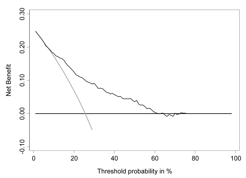
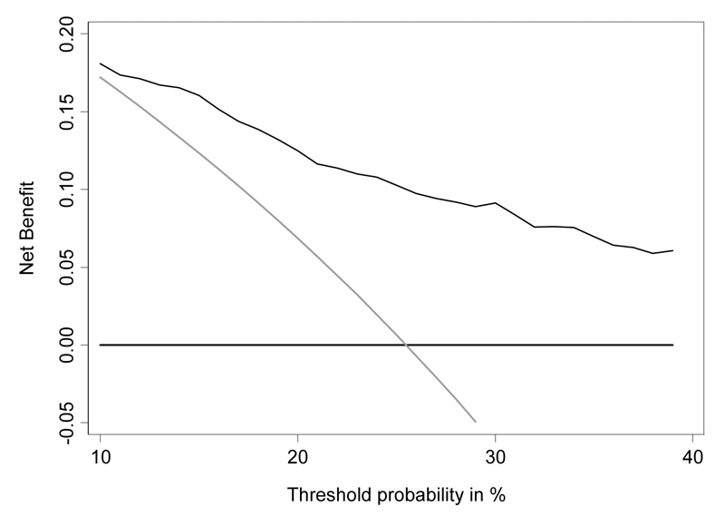
The decision curve for free-to-total PSA is shown in Figure 3. To interpret the decision curve, we need an estimate of the range of threshold probabilities in typical patients. We can obtain such an estimate from clinicians: a typical response is that few men would opt for biopsy if they were told they had a risk of prostate cancer less than 10%; on the other hand, it is hard to imagine that a man taking a PSA test would want at least a 50:50 chance of cancer before agreeing to biopsy. Figure 4 shows the decision curve for free-to-total PSA ratio in our reasonable range of 10 – 40%. Net benefit is superior to biopsying all or no men across the whole range. We can therefore conclude that using free-to-total PSA ratio to determine biopsy in men with elevated PSA will improve clinical outcomes irrespective of any differences in patient and physician preferences.

Figure 3.

Decision curve analysis for free-to-total PSA ratio in men with elevated PSA. Grey line: biopsy all men. Thin black line: use free-to-total PSA ratio to determine who to biopsy. Thick black line: biopsy no man.

Figure 4.

Decision curve analysis for free-to-total PSA ratio in men with elevated PSA, showing the critical range of threshold probabilities, 10 – 40%. Grey line: biopsy all men. Thin black line: use free-to-total PSA ratio to determine who to biopsy. Thick black line: biopsy no man.

Note that decision curve analysis does not require that patients be asked about their threshold probability, indeed, our conclusions are independent of the mode of decision making. For example, in the case of prostate cancer biopsy, a clinician has the following options to choosing who to biopsy:

• Set a threshold and apply to all patients: patients above the threshold are biopsied, patients below the threshold are not

• Divide patients into high, low and intermediate risk. High risk patients are biopsied; low risk patients are not. Whether or not to biopsy a patient at intermediate risk is taken on a case by case basis, depending on the patients' age, cormorbidites and personal preference.

• Discuss biopsy with each patient and obtain a quantitative estimate of their personal preferences. Compare this estimate with their risk from the model and act accordingly.

Irrespective of how the physician decides which patients should be biopsied, decision curve analysis shows that using free-to-total ratio will improve decision making, as long as any thresholds used are in the reasonable range of 10 – 40%. Hence decision curve analysis can be applied to a data set without the need to obtain the sort of additional information - such as on the benefits of treatment, or subjective patients preferences – typically required by traditional decision analysis; all that is required is a general estimate for a reasonable range of threshold probabilities.

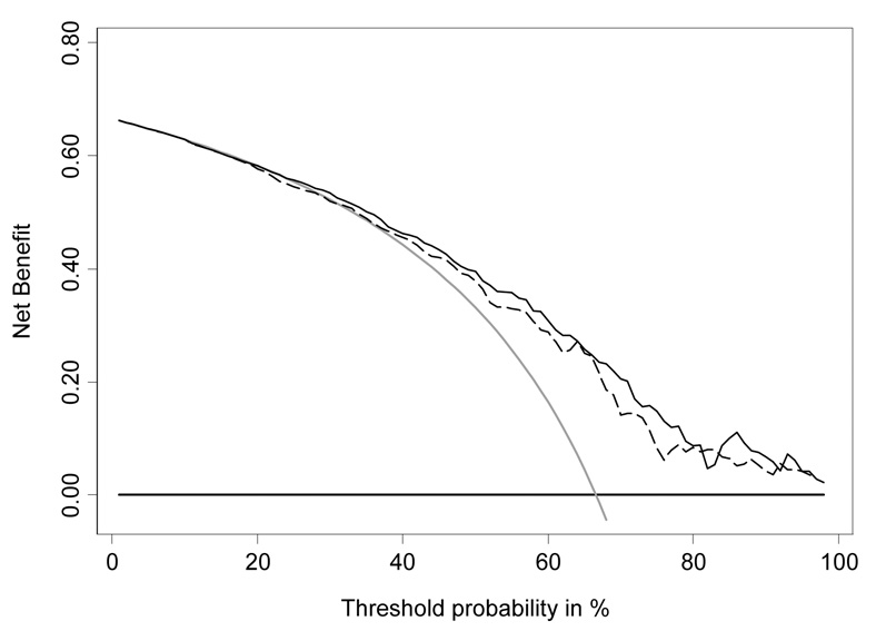
Figure 5 shows a decision curve for a different marker, evaluated on a different set of patients. This demonstrates two points about decision curve analysis. First, the method can be used to evaluate the marginal value of a molecular marker, by estimating the net benefit of a statistical model including both standard predictors and the new marker with that of the standard predictors alone. Second, decision curve analysis can determine that a model is not of clinical value despite good accuracy. The AUC of the model including urokinase was excellent (0.751) and yet it clearly has minimal clinical value: in the critical range of threshold probabilities of 10 – 40%, net benefit is no higher than the strategy of biopsying all patients. This is no doubt related to the extremely high prevalence of prostate cancer in this data set (~65%).

Figure 5.

Decision curve analysis for urokinase. Grey line: biopsy all men. Thick black line: biopsy no man. Dashed line: biopsy men on the basis of a statistical model incorporating age and PSA level. Thin black line: biopsy men on the basis of a statistical model incorporating age, PSA level and urokinase.

Conclusions

The biostatistical literature has almost exclusively been concerned with methods for evaluating the accuracy of predictive models, diagnostic tests and molecular markers. While novel approaches assessing ROC curves, classification tables or calibration continue to proliferate, methods that incorporate clinical consequences are almost entirely absent from the literature. The clinical literature is similarly marked by a near exclusive focus on accuracy. We recently reviewed 129 molecular marker studies in cancer, and although we found that many studies did evaluate whether or not a marker was accurate, not a single study used decision analytic methods to determine whether the marker would improve clinical outcome (Vickers et al. 2008).

Accuracy metrics clearly have their place. In the early phases of research, assessment of accuracy can help determine whether a test, model or marker is sufficiently promising to warrant further testing, and can help refine techniques before a definitive study. As a trivial example, evidence of miscalibration might prompt an analyst to explore the use of non-linear terms or a Bayesian correction factor. Moreover, it would surely be overly pragmatic to claim that a decision-analytic approach is all that is required, and that evaluation of accuracy does not aid our understanding of a test, model or marker that we wish to bring to clinical practice.

Nonetheless, I have argued here that thinking only in terms of accuracy is limited. We need to know not only whether a diagnostic test, predictive model or molecular marker is accurate, but whether it is helpful clinically. As such, I would argue for increased attention to decision-analytic techniques in the methodologic and clinical literature. In particular, analysts should consider methods that can be based on general clinical estimates, but which can provide insight into the consequences of using a test, model or marker in the clinic. These methods involve only the most trivial of computations and are thus straightforward to implement in biostatistical practice.

References

- Baker SG, Kramer B. Peirce, Youden and receiver operating characteristic curves. The American Statistician. 2007;6:1–4. [Google Scholar]
- Berry DA, Parmigiani G. Assessing the benefits of testing for breast cancer susceptibility genes: a decision analysis. Breast Dis. 1998;10:115–125. doi: 10.3233/bd-1998-101-213. [DOI] [PubMed] [Google Scholar]
- Hunink M, Glasziou P, Siegel J. Decision-Making in Health and Medicine: Integrating Evidence and Values. New York: Cambridge University Press; 2001. [Google Scholar]
- Marchionni L, Wilson RF, Wolff AC, Marinopoulos S, Parmigiani G, Bass EB, Goodman SN. Systematic review: gene expression profiling assays in early-stage breast cancer. Ann Intern Med. 2008;148:358–369. doi: 10.7326/0003-4819-148-5-200803040-00208. [DOI] [PubMed] [Google Scholar]
- Pauker SG, Kassirer JP. The threshold approach to clinical decision making. N Engl J Med. 1980;302:1109–1117. doi: 10.1056/NEJM198005153022003. [DOI] [PubMed] [Google Scholar]
- Roddam AW, Duffy MJ, Hamdy FC, Ward AM, Patnick J, Price CP, Rimmer J, Sturgeon C, White P, Allen NE. Use of prostate-specific antigen (PSA) isoforms for the detection of prostate cancer in men with a PSA level of 2–10 ng/ml: systematic review and meta-analysis. Eur Urol. 2005;48:386–399. doi: 10.1016/j.eururo.2005.04.015. [DOI] [PubMed] [Google Scholar]
- Schroder FH, Denis LJ, Roobol M, Nelen V, Auvinen A, Tammela T, Villers A, Rebillard X, Ciatto S, Zappa M, Berenguer A, Paez A, Hugosson J, Lodding P, Recker F, Kwiatkowski M, Kirkels WJ. The story of the European Randomized Study of Screening for Prostate Cancer. BJU Int. 2003;92 Suppl 2:1–13. doi: 10.1111/j.1464-410x.2003.04389.x. [DOI] [PubMed] [Google Scholar]
- Skates SJ, Xu FJ, Yu YH, Sjövall K, Einhorn N, Chang Y, Bast RC, Jr, Knapp RC. Toward an optimal algorithm for ovarian cancer screening with longitudinal tumor markers. Cancer. 1995;76(10 Suppl):2004–2010. doi: 10.1002/1097-0142(19951115)76:10+<2004::aid-cncr2820761317>3.0.co;2-g. [DOI] [PubMed] [Google Scholar]
- Vergouwe Y, Steyerberg EW, Eijkemans MJ, Habbema JD. Validity of prognostic models: when is a model clinically useful? Semin Urol Oncol. 2002;20:96–107. doi: 10.1053/suro.2002.32521. [DOI] [PubMed] [Google Scholar]
- Vickers A, Jang K, Sargent D, Lilja H, Kattan M. A systematic review of statistical methods used in molecular marker studies in cancer. Cancer. 2008;112(8):1862–1868. doi: 10.1002/cncr.23365. [DOI] [PMC free article] [PubMed] [Google Scholar]
- Vickers AJ, Elkin EB. Decision curve analysis: a novel method for evaluating prediction models. Med Decis Making. 2006;26:565–574. doi: 10.1177/0272989X06295361. [DOI] [PMC free article] [PubMed] [Google Scholar]