Abstract
In non-rigid registration, the tradeoff between warp regularization and image fidelity is typically determined empirically. In atlas-based segmentation, this leads to a probabilistic atlas of arbitrary sharpness: weak regularization results in well-aligned training images and a sharp atlas; strong regularization yields a “blurry” atlas.
In this paper, we employ a generative model for the joint registration and segmentation of images. The atlas construction process arises naturally as estimation of the model parameters. This framework allows the computation of unbiased atlases from manually labeled data at various degrees of “sharpness”, as well as the joint registration and segmentation of a novel brain in a consistent manner.
We study the effects of the tradeoff of atlas sharpness and warp smoothness in the context of cortical surface parcellation. This is an important question because of the increasingly availability of atlases in public databases and the development of registration algorithms separate from the atlas construction process. We find that the optimal segmentation (parcellation) corresponds to a unique balance of atlas sharpness and warp regularization, yielding statistically significant improvements over the FreeSurfer parcellation algorithm. Furthermore, we conclude that one can simply use a single atlas computed at an optimal sharpness for the registration-segmentation of a new subject with a pre-determined, fixed, optimal warp constraint. The optimal atlas sharpness and warp smoothness can be determined by probing the segmentation performance on available training data. Our experiments also suggest that segmentation accuracy is tolerant up to a small mismatch between atlas sharpness and warp smoothness.
Keywords: Generative Model, Registration, Segmentation, Parcellation, Multiple Atlases, Markov Random Field, Regularization
1 Introduction
In this work, we propose a generative model for the joint registration and parcellation of cortical surfaces. We formulate the atlas construction process as estimation of the generative model parameters. This provides a consistent framework for constructing the atlas as well as the registration and segmentation of a novel subject. We explore the effects of registration regularization on the atlas construction and the new image segmentation. We conclude that optimal segmentation corresponds to a unique balance of atlas sharpness and warp regularization. However, the segmentation accuracy is tolerant up to a small mismatch between atlas sharpness and warp smoothness.
1.1 Probabilistic Atlases
Probabilistic atlases are powerful tools in segmentation [3,7,11,16,17,35,44]. The simplest probabilistic segmentation atlas provides only the prior probability of labels at a spatial position and no information about the expected appearance of the image. One uses this type of atlas to initialize and to guide the segmentation of a new image [44]. More sophisticated algorithms deform the atlas to the new image and transfer label probabilities from the atlas to the image [3,21]. These label probabilities are then combined with the inten-sity of the new image to produce the final segmentation. We note that the phrase “image intensities” is used in a generic sense to indicate all image-derived features, such as MR intensity or cortical geometry. In this approach, the relationship between labels and image intensities is estimated in the new image and not from the training images used to compute the atlas.
More complex probabilistic atlases provide statistics on the relationship between the segmentation labels and the image intensities [11,12,16,17,35]. The intensity model in the atlas is used to bring the atlas and new image into the same space. The label probabilities and intensity model are then used to segment the new image. Such a registration process can be done sequentially [11,16,17] or jointly [35]. Since this complex atlas contains more information than the simpler atlas, it can conceivably be a more powerful tool for segmentation. However, extra care is needed if the modalities of the new image and training images are different.
In this work, we focus on probabilistic segmentation atlases that model both labels and intensities. An initial step in probabilistic atlas computation is the spatial normalization of the training images. The features used for co-registering images are usually derived from the images themselves [1,4,13,20,23,25,34,43] or from the segmentation labels [10,29,45,46,51]. After normalization to a common space, we can compute the variability in intensity values (and/or labels) in the atlas space. Our approach uses both labels and intensities to co-register the training images. The need to utilize both labels and intensities arises naturally from the proposed generative model.
Joint registration-segmentation algorithms are generally more effective than sequential registration-segmentation as registration and segmentation benefit from additional knowledge of each other [3,35,47–50]. In our case, the requirement to jointly register and segment is also a natural consequence of the generative model.
1.2 Warp Regularization
Spatial normalization of the training images can be achieved with different registration algorithms that vary in the flexibility of warps they allow. Both low-dimensional warps, e.g., affine [35], and richer, more flexible warps can be employed, e.g., splines [4,43,46], dense displacement fields [10,20,13,17,45] and velocity fields [23,29]. More restricted warps yield blurrier atlases that capture inter-subject variability of structures, enlarging the basin of attraction for the registration of a new subject. However, label prediction accuracy is limited by the sharpness of the atlas. Recently, it has been shown that combining information on the warp flexibility and the residual image of the registration process improve the classification accuracy of schizophrenic and normal subjects [30]. Finding the optimal warp regularization tradeoff has received attention in recent years. Twining et al. [43] and Van Leemput [45] propose frameworks to find the least complex models that explain the image intensity and segmentation labels of the training images.
In contrast, we explicitly explore the relationship between the warp flexibility and the atlas sharpness in the context of atlas-based segmentation. Rather than finding one optimal warp regularization when computing the atlas, we compute atlases with varying degrees of warp regularization and thus obtain atlases of varying degrees of sharpness. We use these to study the effect of atlas sharpness and warp regularization on segmentation accuracy. In particular, we compare three specific approaches: (1) progressive (i.e., using increasingly flexible warps) registration-segmentation of a new brain with increasingly sharp atlases; (2) progressive registration with an atlas of a particular sharpness; (3) registration with an atlas of a particular sharpness using a pre-determined, fixed constraint on the warp.
1.3 Cortical Parcellation
We investigate the question of regularization in the context of automatic parcellation of cortical surfaces. Automatic labeling of surface models of the cerebral cortex is important for identifying regions of interest for clinical, functional and structural studies [11,39]. In particular, it has been shown that cortical surface registration can increase the power of functional alignment or activation consistency [14], as well as the alignment of cytoarchitectonics [18]. Recent efforts range from identification of sulcal or gyral ridge lines [41,42] to segmentation of sulcal or gyral basins [11,17,27,28,31,37,39]. Similar to these prior studies, we are interested in the parcellation of the entire cortical surface, i.e., the automated labeling of each point of the surface of a new subject.
Because the local geometries of different sulci and gyri might be similar, learning the geometries of the different sulcal and gyral labels using information from a new image only is difficult. Instead, we will follow the approach of [17,11] and utilize an atlas that encodes both the spatial distributions of the labels and their spatially varying geometries.
In the context of cortical parcellation, our experiments suggest that the optimal parcellation in all three registration schemes for exploring atlas sharpness and warp regularization corresponds to a unique balance of atlas sharpness and warp regularization. Furthermore, the optimal parameters yield statistically significant improvements over the FreeSurfer parcellation algorithm [17]. There is no difference in the optimal parcellation accuracy achieved by the three schemes.
While one might expect that outlier images require weaker regularization to warp closer to the population “average” to achieve better segmentation accuracy, our experiments show that it is sufficient to use a single atlas computed at an optimal sharpness for the registration-segmentation of a new subject with a pre-determined, fixed, optimal warp constraint.
The optimal atlas sharpness and warp smoothness can be determined by probing the segmentation performance on available training data. We find that the optimal warp smoothness for the new subject should be the same as the warp smoothness used for creating the atlas. While this might be an obvious consequence of our explicit generative model, in practice, it is common to use or develop a registration algorithm separate from atlas construction. This is especially true with the increasing availability of atlases in publicly available databases, such as MNI305 [12]. It is therefore important to determine whether using different warp smoothness and atlas sharpness is necessarily detrimental to segmentation in practice. Our experiments suggest that segmentation accuracy is tolerant up to a small mismatch between atlas sharpness and warp smoothness.
A preliminary version of this work was published at the International Conference on Medical Image Computing and Computer Assisted Intervention [52]. This article expands the conference paper with a more detailed theoretical development and more extensive experimental work. In particular, the theory for the atlas construction process was only briefly discussed in [52], but is covered in depth in this paper.
Our contributions are as follows:
We propose a generative model for the joint registration and segmentation of images. The atlas construction process is formulated as a parameter estimation problem. This provides a consistent framework for both estimating the atlas, as well as for the registration and segmentation of a new image.
We explore the space of atlas sharpness and warp regularization for registering and parcellating cortical surfaces. We find that the optimal parcellation corresponds to a unique balance of atlas sharpness and warp regularization. The robustness of the optimal atlas sharpness and warp regularization across trials suggests that we can use the same parameters for future cortical surface parcellation.
We show improved parcellation results over the state-of-the-art FreeSurfer parcellation algorithm [17].
In the next section, we introduce the generative model, describe the resulting atlas estimation process, and the registration and segmentation of a novel image. Section 3 introduces the cortical surface parcellation problem and describes further modeling assumptions made in the context of this problem. We present experimental results in Section 4.
2 Theory
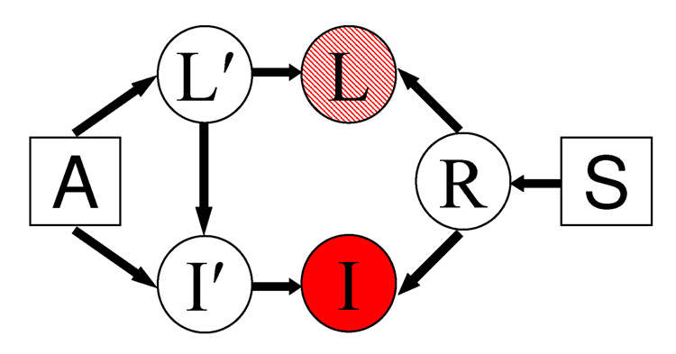
Given a training set of N images I1:N = {I1, …, IN} with label maps L1:N = {L1, …, LN}, joint registration-segmentation aims to infer the registration parameters R and segmentation labels L of a new image I. To achieve this goal, we first learn the parameters of the generative model (Figure 1) from the training images. These parameters correspond to the atlas A and smoothness parameter S. Here, we assume the generative model for the warp R is parameterized by S. According to the generative model, the parameters R and A are independent. However, conditioned on the observed image, R and A become dependent. Estimating the parameters S and A involves co-registration of the training images into a common space. We emphasize that our co-registration process uses both the labels and image intensities of the training images, as described in the next section.
Fig. 1.
Generative model for registration and segmentation. A is an atlas used to generate the label map L′ in some universal atlas space. The atlas A and label map L′ generate image I′. S is the smoothness parameter that generates random warp field R. This warp is then applied to the label map L′ and image I′ to create the label map L and the image I. We assume the label map L is available for the training images, but not for the test image. The image I is observed in both training and test cases.
2.1 Generative Model for Registration and Segmentation
We consider the generative model of Figure 1. L′ is a label map in the atlas space generated probabilistically by the atlas A. For example, L′ could be the tissue type at each MRI pixel, generated by a tissue probability map. Given the label map, the atlas then generates image I′. For example, at each pixel, we can generate an MR intensity conditioned on the tissue type and spatial location. Finally, we generate a random warp field R controlled by the smoothness parameter S. For example, we can generate a random displacement field, with neighboring displacements encouraged to be “close”. For example, S can be the spacing of spline control points or the penalty in a cost function that discourages large or discontinuous deformation fields. The random warp R is then applied to the label map L′ and image I′ to create the observed label map L and observed image I, i.e., I(R(x)) = I′(x) and L(R(x)) = L′(x). Thus a location x in the atlas space is mapped to a location R(x) in the native (or raw) image space. We defer a detailed instantiation of the model to Section 3.
During co-registration, a small value of smoothness parameter S leads to less constrained warps, resulting in better alignment of the training images3. This results in a sharper atlas. On the other hand, a larger smoothness parameter yields more regularized warps and a blurrier atlas.
2.2 Atlas Building: Estimating Parameters of Generative Model
To estimate the parameters of the generative model, we maximize the likely-hood of the observed images I1:N and L1:N over the values of the non-random smoothness parameter S and atlas A.
| (1) |
| (2) |
Here p(a; b) indicates the probability of random variable a parameterized by a non-random parameter b while p(a|b) indicates the probability of random variable a conditioned on a random variable b.
In this case, we need to marginalize over the registration warps R1:N, which is difficult. Previously demonstrated methods for atlas construction use various approximations to evaluate the integral. In this paper, we adopt the standard approximation that replaces the integral with the value of the integrand estimated at the maximum likelihood estimate of deformation. In contrast, [38] uses a sampling method while [45] uses the Laplace approximation, which essentially models the distribution to be a Gaussian centered at the maximum likelihood estimate. It is unclear that these more complex methods, while theoretically more sound, lead to (practically) better approximation. Based on this approximation, we seek
| (3) |
| (4) |
| (5) |
The second equality comes from the fact that the training images are independent of each other given the atlas A and smoothness parameter S. The last equality is obtained by applying Bayes’ rule and the independence relations specified by the graphical model in Figure 1.
Optimizing the above expression yields the atlas A* and smoothness parameter S*. As mentioned before, a smaller value of the smoothness parameter S results in a sharper atlas. Since we are interested in how atlas sharpness affects segmentation accuracy, instead of estimating one single optimal S*, we construct a series of atlases corresponding to different values of the regularization parameter S. In particular, we discretize S into a finite set {Sk} = {S1 > S2 > … > SK}. For each value Sk, we seek the optimal atlas and set of deformations:
| (6) |
We shall refer to the atlas computed using a particular Sk as Aα=Sk. We use alternating optimization to maximize Eq. (6). In each step, we fix the set of registration warps R1:N and estimate the atlas Aα=Sk:
| (7) |
We then fix the atlas Aα=Sk, and optimize the registration warps R1:N by optimizing each warp independently of others:
| (8) |
This process is repeated until convergence. Convergence is guaranteed since this is essentially a coordinate-ascent procedure operating on a bounded function.
We can think of Eq. (8) as the atlas co-registration objective function by treating log p(In, Ln|Rn;ASk) as the data fidelity function and log p(Rn; Sk) as the regularization term. We effectively register each image independently to the atlas Aα=Sk. This iterated process of updating the atlas is similar to [23], except we include training labels in the co-registration. We will show a concrete instantiation of this formulation in Section 3.
In practice, we first create atlas A∞ based on a simple rigid-body registration and use it to initialize the atlas AS1, where S1 is large enough such that the resultant warp is almost rigid. We then use atlas AS1 to initialize the atlas AS2 where S1 > S2, and so on. The result is a set of atlases {Aα} = {AS1 … ASK}. With enough samples, the finite set {Sk,Aα =Sk} accurately represents the underlying continuous space of atlases at different levels of sharpness.
2.3 Registration and Segmentation of a New Image
Given an atlas A and smoothness parameter S, the registration and segmentation of a new image I can be computed using a Maximum-A-Posteriori (MAP) estimate. This involves finding the mode of the posterior distribution of the new image labels L and registration R given the observed image I and atlas A and smoothness parameter S:
| (9) |
| (10) |
| (11) |
The second equality follows from the definition of the conditional probability. The last equality follows from the independence relations specified by the graphical model in Figure 1. In prior work, this MAP approach is favored by some [47–49], while others suggest estimating the MAP solution for the registration warp alone [3,35]:
| (12) |
| (13) |
and recovering the segmentation labels as a final step after recovering the optimal registration R*. Prior work in joint registration and segmentation did not consider atlas construction in the same framework [3,35,47–49]. Furthermore, S is usually set by an expert rather than estimated from the data.
We previously reported results based on the latter two-step approach [52]. In this version, we use the former MAP framework since it requires fewer assumptions for practical optimization. As we show in Section 3, optimizing Eq. (11) using a soft-MAP coordinate ascent approach using the Mean Field approximation [22,26] results in the same update rule used by our previously demonstrated method [52].
The differences between the new image registration specified by Eq. (11) and the atlas co-registration objective function in Eq. (8) comes from the unavoidable fact that for the new image, the label map is not observed. To optimize Eq. (11), we use a coordinate ascent scheme. In step t, we fix the registration parameters R(t) and estimate the labels L(t+1):
| (14) |
| (15) |
| (16) |
Eq. (16) optimizes the log posterior probability of the label map L given the image I, atlas A and current estimate of the registration parameters R(t). Next, we fix the label estimate L(t+1) and re-estimate the registration parameters R(t+1):
| (17) |
We can think of Eq. (17) as the new image registration objective function by treating log p(I, L(t+1)|R;A) as the data fidelity term and log p(R; S) as the regularization term.
To maintain generality, we allow the use of a smoothness parameter Sk for the registration and segmentation of a new subject with an atlas Aα where Sk may not be equal to α. In other words, we can, for instance, compute an atlas using affine transformations, while using a flexible deformation model for the registration of a new subject. Strictly speaking, Sk should theoretically be equal to α in Eq. (11) from the perspective of probabilistic inference. Here, we examine whether using different warp smoothness and atlas sharpness is necessarily detrimental to segmentation in practice.
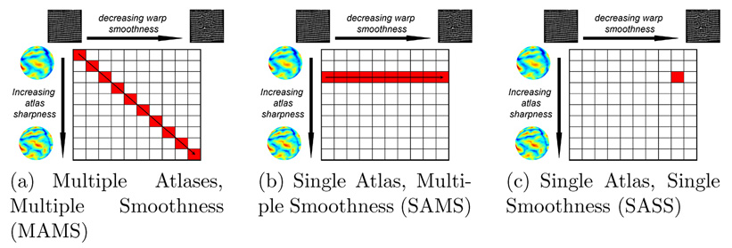
More specifically, we investigate three strategies for exploring the space of atlas sharpness and warp smoothness to register and segment a new image as illustrated in Figure 2.
Multiple Atlas, Multiple Smoothness (MAMS): A multiscale approach where we optimize Eq. (16) and Eq. (17) w.r.t. R and L with the blurry atlas AS1 and warp regularization S1. The resulting alignment is used to initialize the registration with a sharper atlas AS2 and a correspondingly flexible warp regularization S2, and so on (Figure 2a).
Single Atlas, Multiple Smoothness (SAMS): We use a fixed atlas of a fixed sharpness scale ASk to compute R and L according to Eq. (16) and Eq. (17) using a progressively decreasing warp smoothness S (Figure 2b).
Single Atlas, Single Smoothness (SASS):We optimize Eq. (16) and Eq. (17) w.r.t. R and L with a fixed atlas ASk and warp regularization Sm, where Sk might not be equal to Sm (Figure 2c).
Fig. 2.
Strategies for exploring space of atlas sharpness and warp smoothness of a new image.
So far, the derivations have been general without any assumption about the atlases Aα, the prior p(R; Sk) or the image-segmentation fidelity p(I, L|R;Aα). In the next section, we instantiate this approach for a concrete example of cortical surface registration and parcellation.
3 Cortical Surface Parcellation
We now demonstrate the framework developed in the previous section for the joint registration and parcellation of surface models of the cerebral cortex. These surfaces are represented by triangular meshes with a spherical coordinate system that minimizes metric distortion [9,13]. The aim is to register an unlabeled cortical surface to a set of manually labeled surfaces and to classify each vertex of the triangular mesh in terms of the anatomical units. To construct the generative model for this problem, we need to define the prior on the registration parameters p(R; S) and the model for label and image generation p(I, L|R;Aα). In general, our model decisions were inspired by previous work on cortical surface parcellation [13,15,17].
3.1 Generative Model for Registration and Segmentation
We model the warp regularization with an MRF parameterized by S:
| (18) |
where is the distance between vertices i and j under registration R, is the original distance, Ni is a neighborhood of vertex i and Z1(S) is the partition function. Our regularization penalizes percentage metric distortion weighted by a scalar S that reflects the amount of smoothness (rigidity) of the final warp. We choose a percentage metric distortion instead of an absolute metric distortion [13] to ensure that the tradeoff between the regularization and the data fidelity term is invariant to scale in our multi-resolution framework. This is especially important in our work since we explore a large range of warp smoothness parameter S. F(·) ensures invertibility. It is zero if any triangle is folded by warp R and one otherwise. We represent the warp R as a displacement field on the sphere. Therefore, a term like F(R) is necessary. One could replace F(R) with a more sophisticated invertibility prior (e.g., [2,33]) or restrict the space of feasible warps to be the space of diffeomorphisms [23,19].
We first decompose the label and image prior
| (19) |
and impose an MRF prior on the parcellation labels
| (20) |
Here, we use the vectorized MRF notation of [26]. Assuming the total number of labels is M, L(R(xi)) is a column vector of size M × 1 that sums to 1. Each component of L(R(xi)) is an indicator variable. In particular, suppose the image has label m at location R(xi), then L(R(xi)) is zero for all entries, except for the m-th entry, which is equal to 1. It is a common practice to relax the constraint so that L still sums to 1 but the entries might take on fractional values to indicate uncertainty in the segmentation results. Ui(Aα) is a 1xM local potential vector that captures the frequency of label L(R(xi)) at vertex i of the atlas mesh. The MxM compatibility matrix Vij(Aα) reflects the likelihood of two labels at vertices i and j being neighbors. Z2(Aα) is the partition function dependent on the atlas Aα, ensuring the given MRF is a valid probability distribution.
We further assume that the noise added to the mean image intensity at each vertex location is independent, given the label at that location.
| (21) |
where Wi(I(R(xi));Aα) is a 1xM observation potential vector defined at each atlas vertex i. The m-th entry corresponds to the likelihood of observing a particular image intensity or vectors of intensity (in this case, the local surface geometries) at location R(xi) given a particular label m. We assume Wi follows a Gaussian distribution, e.g., given that the post-central gyrus is at location R(xi) of the image, we expect the local curvature and/or sulcal depth I(R(xi)) to follow a Gaussian distribution whose parameters are estimated from the training images.
The collection of model components {Ui, Vij,Wi} define the atlas Aα. Eq. (20) defines an isotropic prior on the labels, which is a simpler model than that used by modern approaches. The FreeSurfer parcellation algorithm uses a spatially varying and anisotropic MRF model [17], whose parameters change dynamically with the geometries of the subject being segmented. An anisotropic MRF improves the parcellation accuracy because the boundaries of certain gyral regions are predicted robustly by the variation in curvature. For example, the boundary between the pre-central and post-central gyrus is the central sulcus. Along the boundary, there is high curvature, while across the boundary, the curvature drops off sharply.
We made the explicit choice of warping an image (interpolating an image) to the atlas space. The alternative of warping the atlas (interpolating the atlas) to image space would require us to interpolate the MRF, which is non-trivial. Interpolating U would result in a change in the partition function, which is exponentially hard to compute. In addition, if we were to use the dynamic model of FreeSurfer, since we have made the choice of warping the subject, this would mean that the model parameters and hence the partition function of the MRF would change during the registration step. FreeSurfer does not have this problem because it does not perform joint registration and segmentation. Therefore, we assume V to be spatially stationary and isotropic and drop the subscripts i, j.
3.2 Atlas Building: Estimating Parameters of Generative Model
Substituting Eq. (18), Eq. (20) and Eq. (21) into the atlas co-registration objective function in Eq. (8), we obtain:
| (22) |
where the first term prevents folding triangles, the second term penalizes metric distortion, the third and fourth terms are the Markov prior on the labels and the last term is the likelihood of the surface geometries given the segmentation labels of the n-th training image.
We can then fix and estimate the atlas parameters Aα = {Ui, V,Wi} using Eq. (7). In practice, we use the naive approach of frequency counts [17] to estimate the clique potentials U, V and the maximum likelihood estimation of the Gaussian likelihood terms W. Appendix B provides the implementation details.
3.3 Registration and Segmentation of a New Image
Similarly, we substitute Eq. (18), Eq. (20) and Eq. (21) into the update rules for the new subject segmentation in Eq. (16) and registration in Eq. (17).
Warping the subject to the atlas, optimization in Eq. (16) with a fixed R(t) involves estimating the segmentation labels at positions R(t)({xi}) of the subject, where {xi} are vertices of the atlas mesh. We will denote this segmentation estimate by L̂(t+1) Eq. (16) becomes
| (23) |
Even with fixed R(t), solving the MAP segmentation Eq. (23) is NP-hard. We adopt the Mean Field approximation [22,26]. We then use the complete approximate distribution provided by the Mean Field solver in optimizing Eq. (17). This approximation effectively creates a soft segmentation estimate at each location R(t)(xi) of the new subject. is a column vector of size M × 1. The m-th component of is the probability of finding label m at location R(t)(xi) of the new subject. To estimate the label L̂(x) at an arbitrary location x in the subject space, we interpolate from L̂(t+1) defined at R(t)({xi}) onto location x.
This optimization procedure leads to fewer local minima since it avoids commitment to the initial estimates obtained through hard thresholding that might be very far from a good solution if the new image is originally poorly aligned to the atlas. Appendix A provides an outline for computing L̂(t+1) via the Mean Field approximation. Warping the subject to the atlas, Eq. (17) becomes:
| (24) |
Further implementation details can be found in Appendix B.
4 Experiments and Discussion
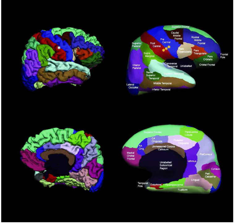
We consider 39 surfaces that represent the gray-white matter interface of the left and right hemispheres automatically segmented from 3D MRI using FreeSurfer [9]. This data set exhibits significant anatomic variability since it contains young, middle-aged, elderly subjects and Alzheimer’s patients. The surfaces are topologically corrected [15,40] and a spherical coordinate system is established by minimizing metric distortion [13]. For each hemisphere, the 39 cortical surfaces are first rigidly aligned on the sphere, which corresponds to rotation only. The surfaces are manually parcellated by a neuroanatomical expert into 35 labels [11]. Figure 3 illustrates the manual parcellation for one subject. A complete list of the parcellation units is included in Table 1.
Fig. 3.
Example of manual parcellation shown on a partially inflated cortical surface. In our data set, the neuroanatomist preferred gyral labels to sulcal labels. There are also regions where sulci and gyri are grouped together as one label, such as the superior and inferior parietal complexes.
Table 1.
List of Parcellation Structures
| 1. | Sylvian Fissure / Unknown | 2. | Bank of the Superior Temporal Sulcus |
| 3. | Caudal Anterior Cingulate | 4. | Caudal Middle Frontal Gyrus |
| 5. | Corpus Callosum | 6. | Cuneus |
| 7. | Entorhinal | 8. | Fusiform Gyrus |
| 9. | Inferior Parietal Complex | 10. | Inferior Temporal Gyrus |
| 11. | Isthmus Cingulate | 12. | Lateral Occipital |
| 13. | Lateral Orbito Frontal | 14. | Lingual |
| 15. | Medial Orbito Frontal | 16. | Middle Temporal Gyrus |
| 17. | Parahippocampal | 18. | Paracentral |
| 19. | Parsopercularis | 20. | Parsorbitalis |
| 21. | Parstriangularis | 22. | Peri-calcarine |
| 23. | Post-central Gyrus | 24. | Posterior Cingulate |
| 25. | Pre-central Gyrus | 26. | Pre-cuneus |
| 27. | Rostral Anterior Cingulate | 28. | Rostral Middle Frontal |
| 29. | Superior Frontal Gyrus | 30. | Superior Parietal Complex |
| 31. | Superior Temporal Gyrus | 32. | Supramarginal |
| 33. | Frontal Pole | 34. | Temporal Pole |
| 35. | Transverse Temporal |
We perform cross-validation by leaving out subjects 1 through 10 in the atlas construction, followed by the joint registration-segmentation of left-out subjects. We repeat with subjects 11 through 20, 21 through 30 and finally 31 through 39.We select S to be the set {100, 50, 25, 12.5, 8, 5, 2.5, 1, 0.5, 0.25, 0.1, 0.05, 0.01}. We find that in practice, S = 100 corresponds to allowing minimal metric distortion and S = 0.01 corresponds to allowing almost any distortion. The intervals in the set S are chosen so that each decrease in the value of S roughly corresponds to an average of 1mm increased displacement in registration.
Since we treat the subject mesh as the moving image, both registration and parcellation are performed on the fixed atlas mesh. The segmentation is interpolated from the atlas mesh onto the subject mesh to obtain the final segmentation. We compute segmentation quality by comparing this final segmentation with the “ground truth” manual parcellation.
To speed up the algorithm, we construct the atlas on a sub-divided icosahedron mesh with about 40k vertices. Typically, each subject mesh has more than 100k vertices. The segmentation labels inferred on the low resolution atlas mesh are therefore computed on a coarser grid than that of the manual parcellation. Yet, as we discuss in the remainder of this section, the proposed implementation on average outperforms the FreeSurfer parcellation algorithm [17].
Despite working with a lower resolution icosahedron mesh, registration at each smoothness scale still takes between 20 minutes to 1.5 hours per subject per atlas. Registration with weakly constrained warps (S ≤ 0.1) requires more time because of the need to preserve the invertibility of the warps. The entire set of experiments took approximately 3 weeks to complete on a computing cluster, using up to 80 nodes in parallel.
4.1 Exploration of Smoothness S and Atlas Aα
In this section, we discuss experimental results for the exploration of the smoothness parameter S and atlases Aα. We measure the segmentation accuracy using the Dice coefficient, defined as the ratio of cortical surface area with correct labels to the total surface area, averaged over the test set.
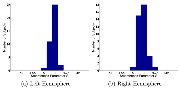
Figure 4 shows the segmentation accuracy for SAMS (Aα = A1) and MAMS as we vary S. The average Dice peaks at approximately S = 1 for all cross-validation trials, although individual variation exists, as shown in Figure 54. For a particular value of S, outliers warp more because the tradeoff between the data-fidelity and regularization is skewed towards the former. However, it is surprising to find that the optimal S is mostly constant across subjects. It also appears that peaks of the segmentation accuracy plots are relatively broad, implying that good parcellation results can be obtained for a range of S between 1 and 2.5.
Fig. 4.
Parcellation accuracy as a function of warp smoothness. S is plotted on a log scale.
Fig. 5.
Histogram of optimal warp smoothness S across subjects (MAMS).
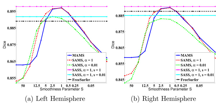
For large S (highly constrained warps), MAMS consistently outperforms SAMS. Because the surfaces are initially misaligned, using a sharp atlas (in the case of SAMS, atlas A1) results in poor segmentation accuracy due to a mismatch between the image features and the atlas statistics. As we decrease the smoothness S, SAMS allows for more flexible warps towards the population average than MAMS since it uses a sharper atlas. The similarity measure is therefore given higher weight to overcome the regularization. This results in better segmentation accuracy than MAMS. Eventually, SAMS and MAMS reach similar maximal values at the same optimal smoothness S. Beyond the optimal S, however, both MAMS and SAMS exhibit degraded performance. This is probably due to overfitting and local optima created by more flexible warps.
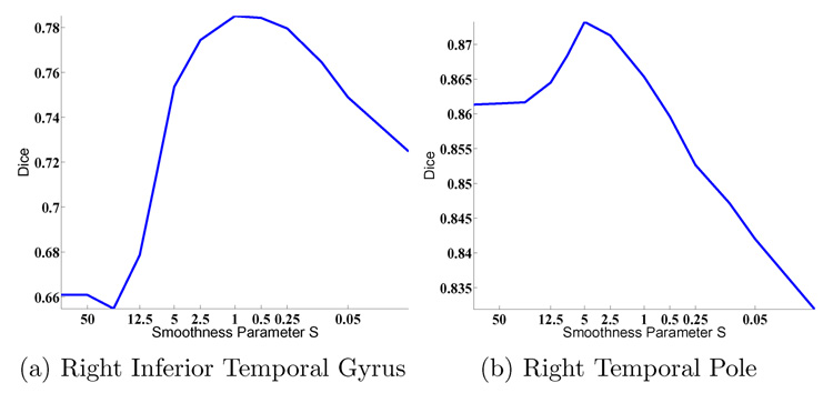
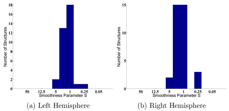
We also examine the Dice measure of each parcellation structure as a function of the warp smoothness S. In general, the curves are noisier but follow those of Figure 4. Figure 6(a) shows a typical curve that peaks at S = 1, while Figure 6(b) shows a curve that peaks at S = 5. However, in general, for most structures, the optimal smoothness S occurs at approximately S = 1 (Figure 7), which is not surprising since for most subjects, the optimal overall Dice (computed over the entire surface) also occurs at S = 1 (Figure 5).
Fig. 6.
(a) Typical plot of Dice against smoothness S. (b) A noisy plot of Dice against smoothness S.
Fig. 7.
Histogram of optimal S across structures (MAMS).
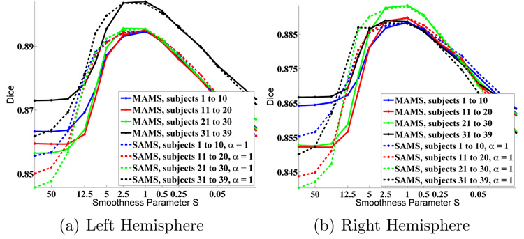
We now explore the effects of both warp smoothness S and atlas sharpness α on parcellation accuracy. Figure 8 shows a plot of Dice averaged over all 39 subjects. The performances of MAMS, SAMS and SASS at (S = 1, α = 1) are indistinguishable. As an example, we see that for both hemispheres, SAMS with α = 0.01 (green line) starts off well, but eventually overfits with a worse peak at S = 1 (p < 10−5 for one-sided paired-sampled t-test, statistically significant even when corrected for multiple comparisons). Similarly for SASS, the best values of α and S are both equal to 1. We also show SASS with α = 0.01 and S = 1 in Figure 8. In general, there is no statistical difference between MAMS, SAMS or SASS at their optima: α = 1, S = 1.
Fig. 8.
Overall Dice versus smoothness. S is plotted on a log scale.
Originally, MAMS and SAMS were introduced to reduce local optima in methods, such as SASS. It is therefore surprising that the performance of all three methods is comparable. While using the correct smoothness and atlas sharpness is important, our “annealing” process of gradual reduction of smoothness (MAMS and SAMS) does not seem to increase the extent of the basins of attraction in the context of cortical parcellation. One possible reason is that on the cortical surfaces, two adjacent sulci might appear quite similar locally. Smoothing these features might not necessarily remove the local minima induced by such similarity. Incorporating multiscale features [32,53,54] with multiple smoothness offers a promising approach for avoiding such local optimal issues on the cortex.
The fact that the optimal smoothness parameter S* corresponds to the optimal atlas sharpness parameter α* is not surprising. According to the graphical model in Figure 1 and as mentioned in the derivations in Section 2.2 and Section 2.3, theoretically, we do expect S* = α*. Learning this optimal S* in the atlas construction process is a future avenue of investigation.
Alternatively, we can also determine the best S and Aα for a new image registration by optimizing the objective function in Eq. (11). Unfortunately, there are technical difficulties in doing this. First, we notice that the objective function in Eq. (11) increases with decreasing S. This model contains no Occam’s razor regularization terms that penalize overfitting due to flexible warps. This is mainly because Eq. (11) omits certain difficult-to-compute normalization terms, such as the partition function that depends on U, V and W and thus dependent on S and α. These terms are ignored for fixed values of S and α. We can use various approximation strategies to compute the normalization terms. But it is not clear whether these approximations yield sufficient accuracy to determine the optimal values for S and α. On the other hand, empirically we find that S = α = 1 consistently yields the optimal (or very close to the optimal) segmentation performance. This suggests that one can probe the training data using a MAMS-type strategy to determine the optimal values of warp smoothness and atlas sharpness, and then use the SASS strategy for future registration and segmentation of new subjects. Furthermore, our experiments suggest that segmentation accuracy is tolerant up to a small mismatch between atlas sharpness and warp smoothness.
Further work will involve the application of our framework to other data sets (including volumetric data) and experiments with other models of data fidelity and regularization. We expect the optimal smoothness and atlas sharpness to be different but it would be interesting to verify if these values are consistent across subjects. It is possible that in the volumetric case where the intensity features are more predictive of labels, a MAMS-type strategy may outperform SASS, particularly in cases where the anatomy is dramatically different (e.g., ventricles in Alzheimer patients).
In this work, the optimal smoothness parameter found is global to the entire surface. Previous work demonstrated the advantage of using spatially varying smoothness parameters [8]. Unfortunately, the approach of exhaustive search presented here cannot be directly applied, since it would involve searching over a much larger space of parameters.
4.2 Comparison with FreeSurfer
We now compare the performance of our algorithm with the FreeSurfer parcellation algorithm, described in [17] and extensively validated in [11].
It is unclear which algorithm has a theoretical advantage. The FreeSurfer algorithm is essentially a “Single Atlas, Single Smoothness” (SASS) method that uses a sequential registration-segmentation approach and a more complicated anisotropic MRF model that has been specifically designed and fine-tuned for the surface parcellation application. Our model lacks the anisotropic MRF and introducing it would further improve its performance. On the other hand, FreeSurfer uses Iterated Conditional Modes [5] to solve the MRF, while we use the more powerful Mean Field approximation [22,26]. FreeSurfer also treats the subject mesh as a fixed image and the parcellation is performed directly on the subject mesh. Therefore, unlike our approach, no interpolation is necessary to obtain the final segmentation.
As shown in Figure 8, the optimal performances of MAMS, SAMS and SASS are statistically significantly better (even when corrected for multiple comparisons) than the FreeSurfer, with p-value 1 × 10⁻⁸ (SASS) for the left hemi- sphere and 8×10⁻⁴ (SASS) for the right hemisphere.
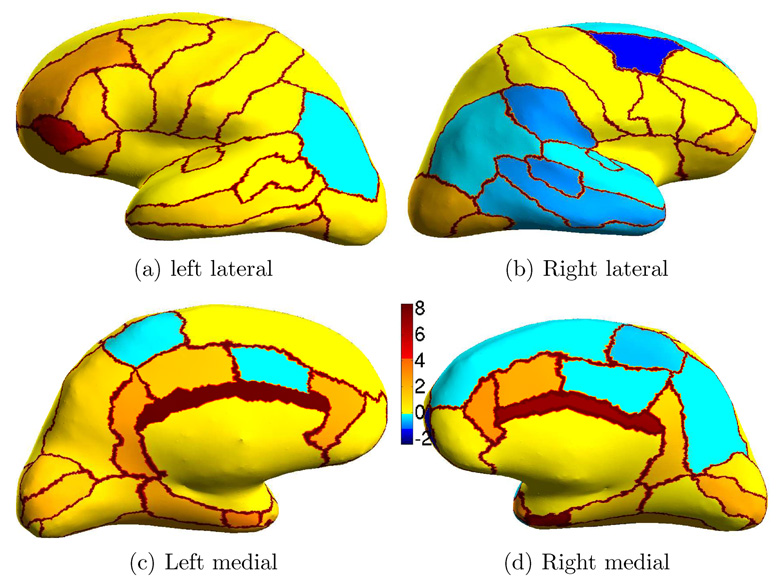
Because Dice computed over the entire surface can be deceiving by suppressing small structures, we show in Figure 9 the percentage improvement of SASS over FreeSurfer on inflated cortical surfaces. Qualitatively, we see that SASS performs better than FreeSurfer since there appears more orange-red regions than blue regions. The fact that the colorbar has significantly higher positive values than negative values indicates that there are parcellation regions with significantly greater improvements compared with regions that suffer significant penalties.
Fig. 9.
Percentage improvement of SASS over FreeSurfer. The boundaries between parcellation regions are set to reddish-brown so that the different regions are more visible.
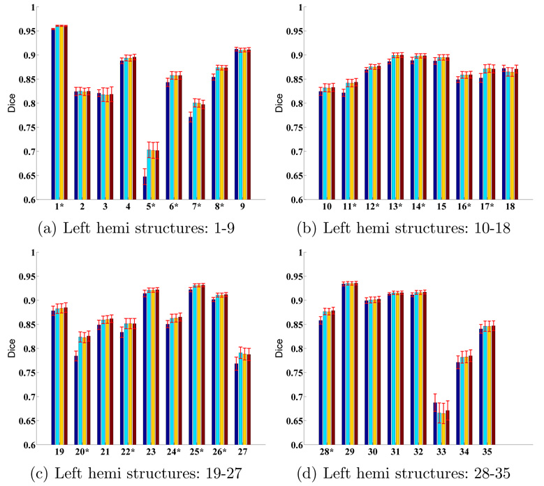
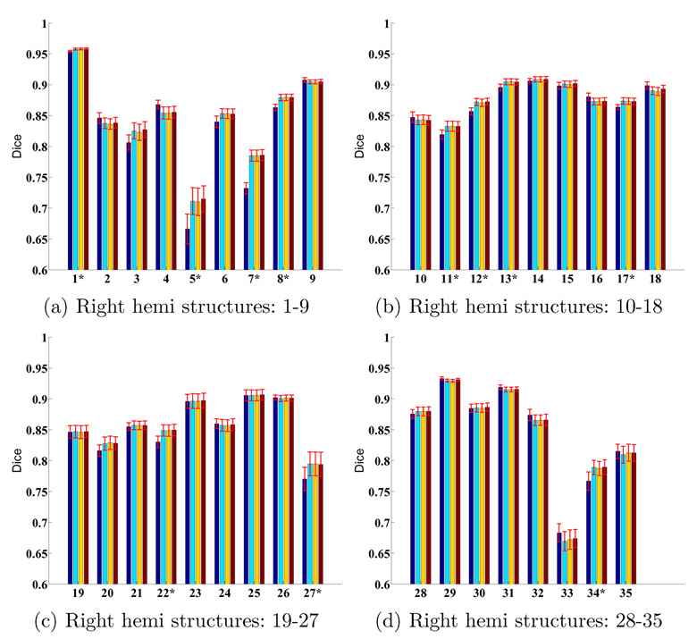
More quantitatively, Figure 10 and 11 display the average Dice per structure for FreeSurfer, MAMS, SAMS and SASS at (S = 1, α = 1) for the left and right hemispheres respectively. Standard errors of the mean are displayed as red bars. The numbering of the structures correspond to Table 1. The structures with the worst Dice are the frontal pole, corpus callosum and entorhinal cortex. These structures are small and relatively poorly defined by the underlying cortical geometry. For example, the entorhinal cortex is partially defined by the rhinal sulcus, a tiny sulcus that is only visible on the pial surface. On the other hand, the corpus callosum is mapped from the white matter volume onto the cortical surface. Its boundary is thus defined by the surrounding structures, rather than by the cortical geometry.
Fig. 10.
Structure-specific parcellation accuracy for the left hemisphere. First column (dark blue) corresponds to FreeSurfer. Second (light blue), third (yellow) and fourth (brown) columns correspond to MAMS, SAMS and SASS respectively. (S = 1, α = 1). * indicates structures where SASS shows statistically significant improvement over FreeSurfer. There is no structure that becomes worse.
Fig. 11.
Structure-specific parcellation accuracy for the right hemisphere. First column (dark blue) corresponds to FreeSurfer. Second (light blue), third (yellow) and fourth (brown) columns correspond to MAMS, SAMS and SASS respectively. (S = 1, α = 1). * indicates structures where SASS shows statistically significant improvement over FreeSurfer. There is no structure that becomes worse.
For each structure, we perform a one-sided paired-sampled t-test between SASS and FreeSurfer, where each subject is considered a sample. We use the False Discovery Rate (FDR) [6] to correct for multiple comparisons. In the left hemisphere, SASS achieves statistically significant improvement over FreeSurfer for 17 structures (FDR < 0.05), while the remaining structures yield no statistical difference. In the right hemisphere, SASS achieves improvement for 11 structures (FDR < 0.05), while the remaining structures yield no statistical difference. The p-values for the left and right hemispheres are pooled together for the False Discovery Rate analysis.
A major factor influencing the accuracy of the automatic parcellation is the manual segmentation. In well-defined regions such as pre- and post-central gyri, accuracy is more than 90% and within the range of inter-rater variability. In the ambiguous regions, such as the frontal pole, inconsistent manual segmentation leads to less consistent training and worse segmentation performance.
5 Conclusions
In this paper, we proposed a generative model for the joint registration and segmentation of images. The atlas construction process is formulated as estimation of the graphical model parameters. The framework incorporates consistent atlas construction, multiple atlases of varying sharpness and MRF priors on both registration warps and segmentation labels. We show that atlas sharpness and warp regularization are important factors in segmentation and that the optimal smoothness parameters are stable across subjects in the context of cortical parcellation. The experiments imply that the optimal atlas sharpness and warp smoothness can be determined by cross-validation. Furthermore, segmentation accuracy is tolerant up to a small mismatch between atlas sharpness and warp smoothness. With the proper choice of atlas sharpness and warp regularization, even with a less complex MRF model, the joint registration-segmentation framework achieves better segmentation accuracy than the state-of-the-art FreeSurfer algorithm [11,17].
There are various promising directions for future work. We believe that incorporating multiscale features [32,53,54] can further improve the registration and parcellation of the cortical surfaces. Learning the optimal spatially varying smoothness parameters in the training set is also a problem we are currently working on. Finally, we plan to apply this framework to other problems, including volumetric segmentation.
A Mean Field Derivation Outline
The mean-field approximation uses a variational formulation [22], where we seek to minimize the KL-divergence (denoted by D(· ∥·)) between q(L̂) = ∏ibi(L̂i) and p(L̂|I(R(t)({xi}));Aα):
| (A.1) |
This results in a fixed-point iterative solution. Since this is a fairly standard derivation [22], we only provide the final update:
| (A.2) |
where bi is normalized to be a valid probability mass function.
B Implementation
We now present some implementation details for completeness.
We first discuss the estimation of the atlas Aα defined by {Ui,V,Wi} in Eq. (20) and Eq. (21) from the maximum likelihood function Eq. (7). In our model, estimating Ui and V is hard in practice, since evaluating Eq. (7) requires computing the NP-hard partition function. Instead, we use frequency counts to estimate the clique potentials, similar to FreeSurfer [17].
- In our implementation, the singleton potential Ui is a row vector of length M and Ln is a column indicator vector. We set
where (·)T indicates transpose.(B.1) The likelihood potential Wi is a row vector of length M defined at each vertex. The m-th entry of Wi corresponds to the likelihood of observing a particular image intensity or vectors of intensity (in our case, the local surface geometries) at location R(xi) given a particular label m. While we might be observing multiple geometric features at any vertex, the likelihood of these features is combined into the row vector Wi. We use maximum likelihood estimates of the mean and variance of the Gaussian distribution of cortical geometries conditioned on the segmentation labels to parameterize this distribution. In this work, we use the mean curvature of the original cortical surface and average convexity, which is a measure of sulcal depth [13], as intensity features.
At spatial locations where there is no training data for a particular label, it is unclear what the value of the entry in W should be since it is spatially varying. We simply assume a mean of zero and a large variance, essentially being agnostic in the value of intensity we observe. A more sophisticated method would involve the use of priors on the atlas parameters, so that the atlas parameters become random. In that case, when there is no observations, the maximum likelihood estimates of the atlas parameters become the priors.
Secondly, we discuss the registration of a training image to an atlas (Eq. (22)) and the new image registration (Eq. (24)).
The registration warp R is a map from a 2-Sphere to a 2-Sphere. We represent R as a dense displacement field. In particular, each point xi has an associated displacement vector ui tangent to the point xi on the sphere. R(xi) maps xi to xi + ui normalized to be a point on the sphere.
To interpolate (for example the mean curvature of a cortical surface onto R(xi)), we first find the intersection between the vector R(xi) and each planar triangle of the spherically mapped cortical surface. We then use barycentric interpolation to interpolate the values at the vertices of the mesh onto R(xi).
The above two bullets completely specify the computation of the atlas co-registration objective function Eq. (22) and the new subject registration function Eq. (24). This allows us to compute the gradients of the objective function via the chain rule.
We use conjugate gradient ascent with parabolic line search [36] on a coarse-to-fine grid. The coarse-to-fine grid comes from the representation of the atlas as a subdivided icosahedron mesh.
The final segmentation is obtained by selecting for each vertex the label with the highest posterior probability.
To satisfy F(R), the regularization that induces invertibility, we ensure that no step in the line search results in folded triangles. Unfortunately, in practice, this results in many small steps. It is much more efficient to perform the line search without considering F(R), and then unfold the triangles using F(R) after the line search. In general, we find that after unfolding, the objective function is still better than the previous iteration. This unfolding process can be expensive for small smoothness parameter S (S ≤ 0.1), resulting in long run times of about 1.5 hours per subject per atlas for S ≤ 0.1.
Acknowledgments
The authors would like to thank Serdar Balci, Wanmei Ou, Kilian Pohl and Lilla Zollei for helpful conversations. They would like to especially thank Koen Van Leem-put for illuminating discussions on atlas construction and other issues in registration. Support for this research is provided in part by the National Alliance for Medical Image Analysis (NIH NIBIB NAMIC U54-EB005149), the Neuroimaging Analysis Center (NIT CRR NAC P41-RR13218), the Morphometry Biomedical Informatics Research Network (NIH NCRR mBIRN U24-RR021382), the NIH NINDS R01- NS051826 grant, the NSF CAREER 0642971 grant, National Center for Research Resources (P41-RR14075, R01 RR16594-01A1 and the NCRR BIRN Morphomet-ric Project BIRN002, U24 RR021382), the National Institute for Biomedical Imaging and Bioengineering (R01 EB001550, R01EB006758), the National Institute for Neurological Disorders and Stroke (R01 NS052585-01) as well as the Mental Illness and Neuroscience Discovery (MIND) Institute. B.T. Thomas Yeo is funded by the Agency for Science, Technology and Research, Singapore.
Footnotes
Publisher's Disclaimer: This is a PDF file of an unedited manuscript that has been accepted for publication. As a service to our customers we are providing this early version of the manuscript. The manuscript will undergo copyediting, typesetting, and review of the resulting proof before it is published in its final citable form. Please note that during the production process errors may be discovered which could affect the content, and all legal disclaimers that apply to the journal pertain.
By a “better alignment of images”, we mean that the warped images look more similar, i.e., the similarity measure is improved. However, an improved similarity measure does not necessarily imply deformations with better label alignment. In fact, we show in the paper that the best segmentation occurs when warps are not overly flexible.
The optimal value of S = 1 is coincidental in the sense that it depends on the unit chosen for metric distortion.
References
- 1.Allassonnière S, Amit Y, Trouvé A. Towards a coherent statistical framework for dense deformable template estimation. Journal of the Royal Statistiscal Society B. 2007;68:3–29. [Google Scholar]
- 2.Ashburner J, Andersson J, Friston K. High-dimensional Image Registration Using Symmetric Priors. NeuroImage. 1999;9:619–628. doi: 10.1006/nimg.1999.0437. [DOI] [PubMed] [Google Scholar]
- 3.Ashburner J, Friston K. Unified Segmentation. NeuroImage. 2005;26:839–851. doi: 10.1016/j.neuroimage.2005.02.018. [DOI] [PubMed] [Google Scholar]
- 4.Bhatia KK, Hajnal JV, Puri BK, Edwards AD, Rueckert D. Consistent Groupwise Non-Rigid Registration for Atlas Construction. International Symposium on Biomedical Imaging. 2004 [Google Scholar]
- 5.Besag J. On the Statistical Analysis of Dirty Pictures. Journal of Royal Statistical Society B. 1986;48(3):259–302. [Google Scholar]
- 6.Benjamini Y, Hochberg Y. Controlling the False Discovery Rate: A Practical and Powerful Approach to Multiple Testing. Journal of Royal Statistical Society B. 1995;57(1):289–300. [Google Scholar]
- 7.Collins DL, Zijdenbos AP, Baaré WFC, Evans AC. ANIMAL+INSECT: Improved Cortical Structure Segmentation. Information Processing in Medical Imaging. 1999;1613:210–223. [Google Scholar]
- 8.Commowick O, Stefanescu R, Fillard P, Arsigny V, Ayache N, Pennec X, Malandain G. Incorporating Statistical Measures of Anatomical Variability in Atlas-to-Subject Registration for Conformal Brain Radiotherapy; International Conference on Medical Image Computing and Computer-Assisted Intervention; 2005. pp. 927–934. LNCS. [DOI] [PubMed] [Google Scholar]
- 9.Dale A, Fischl B, Sereno M. Cortical Surface-Based Analysis I: Segmentation and Surface Reconstruction. NeuroImage. 1999;9(2):179–194. doi: 10.1006/nimg.1998.0395. [DOI] [PubMed] [Google Scholar]
- 10.De Craene M, du Bois d’Aische A, Macq B, Warfield S. Multi-subject Registration for Unbiased Statistical Atlas Construction; International Conference on Medical Image Computing and Computer-Assisted Intervention; 2004. pp. 655–662. LNCS. [Google Scholar]
- 11.Desikan R, S’egonne F, Fischl B, Quinn B, Dickerson B, Blacker D, Buckner R, Dale A, Maguire P, Hyman B, Albert M, Killiany R. An automated labeling system for subdividing the human cerebral cortex on MRI scans into gyral based regions of interest. NeuroImage. 2006;31:968–980. doi: 10.1016/j.neuroimage.2006.01.021. [DOI] [PubMed] [Google Scholar]
- 12.Evans AC, Collins DL, Mills SR, Brown ED, Kelly RL, Peters TM. 3D statistical neuroanatomical models from 305 MRI volumes; Nuclear Science Symposium and Medical Imaging Conference; 1993. pp. 1813–1817. IEEE Conference Record. [Google Scholar]
- 13.Fischl B, Sereno M, Dale A. Cortical Surface-Based Analysis II: Inflation, Flattening, and a Surface-Based Coordinate System. NeuroImage. 1999;9(2):195–207. doi: 10.1006/nimg.1998.0396. [DOI] [PubMed] [Google Scholar]
- 14.Fischl B, Sereno M, Tootell R, Dale A. High-resolution intersubject averaging and a coordinate system for the cortical surface. Human Brain Mapping. 1999;8(4):272–284. doi: 10.1002/(SICI)1097-0193(1999)8:4<272::AID-HBM10>3.0.CO;2-4. [DOI] [PMC free article] [PubMed] [Google Scholar]
- 15.Fischl B, Liu A, Dale A. Automated Manifold Surgery: Constructing Geometrically Accurate and Topologically Correct Models of the Human Cerebral Cortex. IEEE Transactions on Medical Imaging. 2001;20(1):70–80. doi: 10.1109/42.906426. [DOI] [PubMed] [Google Scholar]
- 16.Fischl B, Salat D, Busa E, Albert M, Dieterich M, Haselgrove C, van der Kouwe A, Killiany R, Kennedy D, Klaveness S, Montillo A, Makris N, Rosen B, Dale A. Whole Brain Segmentation: Automated Labeling of Neuroanatomical Structures in the Human Brain. Neuron. 2002;33(3):341–355. doi: 10.1016/s0896-6273(02)00569-x. [DOI] [PubMed] [Google Scholar]
- 17.Fischl B, van der Kouwe A, Destrieux C, Halgren E, Ségonne F, Salat D, Busa E, Seidman LJ, Goldstein J, Kennedy D, Caviness V, Makris N, Rosen B, Dale A. Automatically Parcellating the Human cerebral Cortex. Cerebral Cortex. 2004;14:11–22. doi: 10.1093/cercor/bhg087. [DOI] [PubMed] [Google Scholar]
- 18.Fischl B, Rajendran N, Busa E, Augustinack J, Hinds O, Yeo BTT, Mohlberg H, Amunts K, Zilles K. Cortical Folding Patterns and Predicting Cytoarchitecture. Cerebral Cortex. 2007 doi: 10.1093/cercor/bhm225. [DOI] [PMC free article] [PubMed] [Google Scholar]
- 19.Glaunès J, Vaillant M, Miller M. Landmark Matching via Large Deformation Diffeomorphisms on the Sphere. Journal of Mathematical Imaging and Vision. 2004;20:179–200. [Google Scholar]
- 20.Guimond A, Meunier J, Thirion J-P. Average Brain Models: A Convergence Study. Computer Vision and Image Understanding. 2000;77(2):192–210. [Google Scholar]
- 21.Heckemann RA, Hajnal J, Aljabar P, Rueckert D, Hammers A. Automatic anatomical brain MRI segmentation combining label propagation and decision fusion. NeuroImage. 2006;33(1):115–126. doi: 10.1016/j.neuroimage.2006.05.061. [DOI] [PubMed] [Google Scholar]
- 22.Jaakkola T. Advanced Mean Field Methods: Theory and Practice. MIT Press; 2000. Tutorial on variational approximation methods. [Google Scholar]
- 23.Joshi S, Davis B, Jomier M, Gerig G. Unbiased Diffeomorphic Atlas Construction for Computational Anatomy. NeuroImage. 2004;23:151–160. doi: 10.1016/j.neuroimage.2004.07.068. [DOI] [PubMed] [Google Scholar]
- 24.Jirousek R, Preucil S. On the effective implementation of the iterative proportional fitting procedure. Computational Statistics and Data Analysis. 1995;19:177–189. [Google Scholar]
- 25.Mazziotta J, Toga A, Evans A, Fox P, Lancaster J. A Probabilistic Atlas of the Human Brain: Theory and Rationale for Its Development The International Consortium for Brain Mapping (ICBM) NeuroImage. 1995;2(2):89–101. doi: 10.1006/nimg.1995.1012. [DOI] [PubMed] [Google Scholar]
- 26.Kapur T, Grimson WEL, Kikinis R, Wells W. Enhanced Spatial Priors for Segmentation of Magnetic Resonance Imagery; International Conference on Medical Image Computing and Computer Aided Intervention; 1998. pp. 457–468. [Google Scholar]
- 27.Klein A, Hirsch J. Mindboggle: a scatterbrained approach to automate brain labeling. NeuroImage. 2005;(24):261–280. doi: 10.1016/j.neuroimage.2004.09.016. [DOI] [PubMed] [Google Scholar]
- 28.Lohmann G, VonCramon DY. Automatic labelling of the human cortical surface using sulcal basins. Medical Image Analysis. 2000;4:179–188. doi: 10.1016/s1361-8415(00)00024-4. [DOI] [PubMed] [Google Scholar]
- 29.Lorenzen P, Prastawa M, Davis B, Gerig G, Bullitt E, Joshi S. Multi-Modal Image Set Registration and Atlas Formation. Medical Image Analysis. 2006;10(3):440–451. doi: 10.1016/j.media.2005.03.002. [DOI] [PMC free article] [PubMed] [Google Scholar]
- 30.Makrogiannis S, Verma R, Karacali B, Davatzikos C. A Joint Transformation and Residual Image Descriptor for Morphometric Image Analysis using an Equivalence Class Formulation. Mathematical Methods in Biomedical Image Analysis. 2006 [Google Scholar]
- 31.Mangin J-F, Frouin V, Bloch I, Régis J, Lopez-Krahe J. Automatic construction of an attributed relational graph representing the cortex topography using homotopic transformations; Proceedings of SPIE; 1994. pp. 110–121. [Google Scholar]
- 32.Nain D, Haker S, Bobick A, Tannenbaum A. Multiscale 3-D Shape Representation and Segmentation Using Spherical Wavelets. IEEE Transactions on Medical Imaging. 2007;26(4):598–618. doi: 10.1109/TMI.2007.893284. [DOI] [PMC free article] [PubMed] [Google Scholar]
- 33.Nielsen M, Johansen P, Jackson AD, Lautrup B. Brownian Warps: A Least Committed Prior for Non-rigid Registration; International Conference on Medical Image Computing and Computer-Assisted Intervention; 2002. pp. 557–564. LNCS. [Google Scholar]
- 34.Paus T, Tomaiuolo F, Otaky N, MacDonald D, Petrides M, Atlas J, Morris R, Evans A. Human Cingulate and Paracingulate Sulci: Pattern, Variability, Asymmetry, and Probabilistic Map. Cerebral Cortex. 1996;6:207–214. doi: 10.1093/cercor/6.2.207. [DOI] [PubMed] [Google Scholar]
- 35.Pohl K, Fisher J, Grimson WEL, Kikinis R, Wells W. A Bayesian model for joint segmentation and registration. NeuroImage. 2006;31:228–239. doi: 10.1016/j.neuroimage.2005.11.044. [DOI] [PubMed] [Google Scholar]
- 36.Press WH, Teukolsky SA, Vetterling WT, Flannery BP. Numerical Recipes in C: The Art of Scientific Computing. 2nd ed. Cambridge, U.K: Cambridge University Press; [Google Scholar]
- 37.Rettmann M, Han X, Xu C, Prince J. Automated Sulcal Segmentation Using Watersheds on the Cortical Surface. NeuroImage. 2002;15:329–344. doi: 10.1006/nimg.2001.0975. [DOI] [PubMed] [Google Scholar]
- 38.Richard F, Samson A, Cuenod C. A SAEM algorithm for the estimation of template and deformation parameters in medical image sequences. preprint MAP5. 2007 Nov [Google Scholar]
- 39.Rivière D, Mangin J-F, Papadopoulos-Orfanos D, Martinez J-M, Frouin V, Régis J. Automatic recognition of cortical sulci of the human brain using a congregation of neural networks. Medical Image Analysis. 2002;6:77–92. doi: 10.1016/s1361-8415(02)00052-x. [DOI] [PubMed] [Google Scholar]
- 40.Ségonne F, Pacheco J, Fischl B. Geometrically Accurate Topology-Correction of Cortical Surfaces Using Nonseparating Loops. IEEE Transactions on Medical Imaging. 2007;26(4):518–529. doi: 10.1109/TMI.2006.887364. [DOI] [PubMed] [Google Scholar]
- 41.Tao X, Prince J, Davatzikos C. Using a Statistical Shape Model to Extract Sulcal Curves on the Outer Cortex of the Human Brain. Transactions on Medical Imaging. 2002;21:513–524. doi: 10.1109/TMI.2002.1009387. [DOI] [PubMed] [Google Scholar]
- 42.Tu Z, Zheng S, Yuille A, Reiss A, Dutton R, Lee A, Galaburda AM, Dinov I, Thompson P, Toga A. Automated Extraction of the Cortical Sulci Based on a Supervised Learning Approach. IEEE Transactions on Medical Imaging. 2007;26(4):541–552. doi: 10.1109/TMI.2007.892506. [DOI] [PubMed] [Google Scholar]
- 43.Twining C, Cootes T, Marsland S, Petrovic V, Schestowitz R, Taylor C. A unified information theoretic approach to groupwise non-rigid registration and model building. Information Processing in Medical Imaging. 2005;9:1–14. doi: 10.1007/11505730_1. [DOI] [PubMed] [Google Scholar]
- 44.Van Leemput K, Maes F, Vandermeulen D, Suetens P. Automated model-based tissue classification of MR images of the brain. IEEE Transactions on Medical Imaging. 1999;18(10):897–908. doi: 10.1109/42.811270. [DOI] [PubMed] [Google Scholar]
- 45.Van Leemput K. Probabilistic Brain Atlas Encoding Using Bayesian Inference; International Conference on Medical Image Computing and Computer Aided Intervention; 2006. pp. 704–711. [DOI] [PubMed] [Google Scholar]
- 46.Weisenfeld N, Warfield S. Simultaneous Alignment and Central Tendency Estimation for Brain Atlas Construction. Workshop on Statistical Registration: Pair-wise and Group-wise Alignment and Atlas Formation. 2007 [Google Scholar]
- 47.Wyatt P, Noble A. MAP MRF Joint Segmentation and Registration. Medical Image Analysis. 2003;7(4):539–552. doi: 10.1016/s1361-8415(03)00067-7. [DOI] [PubMed] [Google Scholar]
- 48.Xiaohua C, Brady M, Rueckert D. Simultaneous Segmentation and Registration for Medical Image; International Conference on Medical Image Computing and Computer Aided Intervention; 2004. pp. 663–670. [Google Scholar]
- 49.Xiaohua C, Brady M, Lo J, Moore N. Simultaneous Segmentation and Registration of Contrast-Enhanced Breast MRI. Information Processing in Medical Imaging. 2005;3565:126–137. doi: 10.1007/11505730_11. [DOI] [PubMed] [Google Scholar]
- 50.Yezzi A, Zollei L, Kapur T. A variational framework for integrating segmentation and registration through active contours. Medical Image Analysis. 2003;7(2):171–185. doi: 10.1016/s1361-8415(03)00004-5. [DOI] [PubMed] [Google Scholar]
- 51.Yeo BTT, Sabuncu M, Mohlberg H, Amunts K, Zilles K, Golland P, Fischl B. What Data to Co-register for Computing Atlases; Proceedings of the International Conference on Computer Vision, IEEE Computer Society Workshop on Mathematical Methods in Biomedical Image Analysis; 2007. [DOI] [PMC free article] [PubMed] [Google Scholar]
- 52.Yeo BTT, Sabuncu M, Desikan R, Fischl B, Golland P. Effects of Registration Regularization and Atlas Sharpness on Segmentation Accuracy; International Conference on Medical Image Computing and Computer Aided Intervention; 2007. pp. 683–691. [DOI] [PMC free article] [PubMed] [Google Scholar]
- 53.Yu P, Grant E, Qi Y, Han X, Ségonne F, Pienaar R, Busa E, Pacheco J, Makris N, Buckner R, Golland P, Fischl B. Cortical Surface Shape Analysis Based on Spherical Wavelets. IEEE Transaction on Medical Imaging. 2007;26(4):582–597. doi: 10.1109/TMI.2007.892499. [DOI] [PMC free article] [PubMed] [Google Scholar]
- 54.Yu P, Yeo BTT, Grant E, Fischl B, Golland P. Cortical Folding Development Study based on Over-Complete Spherical Wavelets; Proceedings of MMBIA: IEEE Computer Society Workshop on Mathematical Methods in Biomedical Image Analysis; 2007. [DOI] [PMC free article] [PubMed] [Google Scholar]


