Variational Bayesian Least Squares: An Application to Brain-Machine Interface Data

Abstract

An increasing number of projects in neuroscience require statistical analysis of high-dimensional data, as, for instance, in the prediction of behavior from neural firing or in the operation of artificial devices from brain recordings in brain-machine interfaces. Although prevalent, classical linear analysis techniques are often numerically fragile in high dimensions due to irrelevant, redundant and noisy information. We develop a robust Bayesian linear regression algorithm that automatically detects relevant features and excludes irrelevant ones, all in a computationally efficient manner. In comparison with standard linear methods, the new Bayesian method regularizes against overfitting, is computationally efficient (unlike previously proposed variational linear regression methods, is suitable for data sets with large amounts of samples and a very high number of input dimensions) and is easy to use, thus demonstrating its potential as a drop-in replacement for other linear regression techniques. We evaluate our technique on synthetic data sets and on several neurophysiological data sets. For these neurophysiological data sets, we address the question of whether EMG data collected from arm movements of monkeys can be faithfully reconstructed from neural activity in motor cortices. Results demonstrate the success of our newly developed method in comparison to other approaches in the literature, and, from the neurophysiological point of view, confirms recent findings on the organization of the motor cortex. Finally, an incremental, real-time version of our algorithm demonstrates the suitability of our approach for real-time interfaces between brains and machines.

1 Introduction

In recent years, there has been growing interest in large scale analyses of brain activity with respect to associated behavioral variables. For instance, projects can be found in the area of brain-machine interfaces, where neural firing is directly used to control an artificial system like a robot [4, 15, 22, 29, 30, 36], or where non-invasive brain signals serve to either control a cursor on computer screen [44] or to classify visual stimuli presented to a subject [14, 21]. In such scenarios, the brain signals to be processed are typically high dimensional, on the order of hundreds or thousands of inputs, with large numbers of redundant and irrelevant signals. Linear modeling techniques like linear regression are among the primary analysis tools for such data [22, 27, 42]. However, the computational problem of data analysis not only involves data fitting, but also requires that the model extracted from the data has good generalization properties. This issue is crucial for predicting behavior from future neural recordings, e.g., for continual on-line interpretation of brain activity to control prosthetic devices or for longitudinal scientific studies of information processing in the brain. Surprisingly, robust linear modeling of high-dimensional data is non-trivial as the danger of fitting noise and of encountering numerical problems is high. Classical techniques like ridge regression, stepwise regression, subset selection techniques or Partial Least Squares regression [43] are known to be prone to overfitting and may often require careful human supervision to ensure useful results. Other methods such as Least Absolute Shrinkage and Selection Operator (LASSO) regression [37] attempt to shrink certain regression coefficients to zero, resulting in interpretable models that are sparse. However, LASSO regression has an open parameter that needs to be set either using either n-fold cross-validation or manual hand-tuning.

In this paper, we will focus on how to improve linear data analysis for the high-dimensional scenarios described above, with a view towards developing a "black box" approach that automatically detects the most relevant input dimensions for generalization and excludes other dimensions in a statistically sound way. We are particularly interested in situations where the data contains a very large quantity of samples and the number of input dimensions is very high, as in brain-machine interfaces. For this purpose, we investigate a full Bayesian treatment of linear regression with automatic relevance detection [28] that is computationally efficient and suitable for large amounts of very high-dimensional data. This algorithm can be formulated in closed form with the help of a variational Bayesian approximation, and it introduces “probabilistic backfitting” for linear regression, a key component which contributes greatly towards the algorithm's computational efficiency. Besides several synthetic data evaluations, we apply the algorithm, named Variational Bayesian Least Squares (VBLS) [38], to the reconstruction of EMG data from motor cortical firing from data sets collected by Sergio & Kalaska [34] and Kakei et al. [19, 20]. This data analysis addresses important neurophysiological questions in terms of whether motor cortical neurons can directly predict EMG traces [2, 25, 26, 40, 41], whether motor cortices have a muscle-based topological organization, and whether information in motor cortices should be used to predict behavior in future brain-machine interfaces. Our main focus in this paper is on the statistical analysis of these kinds of data. Comparisons with classical linear analysis techniques and a brute force combinatorial model search (which was executed on a cluster computer) demonstrate that our VBLS algorithm indeed achieves the “black box” quality of a statistical analysis technique that requires no tuning of parameters by the user.

This paper describes in detail the VBLS algorithm and its application to the EMG reconstruction problem by building and extending our prior work in [8, 38]. We discuss the neurophysiological implications of our analyses and present a real-time version of VBLS in order to simulate an application in real-time brain machine interfaces.

2 High Dimensional Regression

Before developing our VBLS algorithm, it is useful to briefly revisit classical linear regression techniques. Assuming there are N observed data samples in the data set $D={\{{\mathbf{x}}_i,y_i\}}_{i=1}^N$ (where ${\mathbf{x}}_i\in {\mathfrak{R}}^{d\times 1}$ are inputs and y_i are scalar outputs), the standard model for linear regression is:

$$y_i=\sum _{m=1}^d{b}_m{x}_{im}+ϵ$$ (1)

where b is the regression vector made up of b_m components, d is the number of input dimensions, and ϵ is additive mean-zero noise. The Ordinary Least Squares (OLS) estimate of the regression vector is b = (X^T X)⁻¹ X^T y, where $\mathbf{X}\in {\mathfrak{R}}^{N\times d}$ consists of vectors x_i arranged in its rows and $\mathbf{y}\in {\mathfrak{R}}^{N\times 1}$ has coefficients y_i. The main problem with OLS regression in high-dimensional input spaces is that the full rank assumption of (X^T X)⁻¹ is often violated due to underconstrained data sets. Ridge regression [16] can “fix” such problems numerically by stabilizing the matrix inversion with a diagonal term (X^T X + αI)⁻¹, but usually introduces uncontrolled bias. Additionally, if the input dimensionality exceeds around 1000 dimensions, the matrix inversion can become prohibitively computationally expensive.

Several ideas exist how to improve over OLS. First, stepwise regression [7] can be employed. However, stepwise regression has been strongly criticized for its potential for overfitting and its inconsistency in the presence of collinearity in the input data [6]. To deal with such collinearity directly, dimensionality reduction techniques like Principal Components Regression (PCR) [24] are useful. These methods retain directions in an input space with large variance, regardless of whether the directions influence the prediction [33], and can even eliminate low variance inputs that may have high predictive power for the outputs [10]. Another class of linear regression methods are projection regression techniques, most notably Partial Least Squares (PLS) regression [43]. PLS regression performs computationally inexpensive O(d) univariate regressions along projection directions, chosen according to the correlation between inputs and outputs. While slightly heuristic in nature, PLS regression is a surprisingly successful algorithm for ill-conditioned and high-dimensional regression problems, although it also has a tendency towards overfitting [33]. There are also more efficient methods for matrix inversion [13, 35], but these methods assume a well-condition regression problem a priori and degrade in the presence of collinearities in inputs. Finally, there is a class of sparsity inducing methods such as LASSO regression [37] that attempt to shrink certain regression coefficients in the solution to zero by using an L1 penalty norm (instead of an L2 penalty norm used by ridge regression). These methods are suitable for high-dimensional data sets, at the expense of requiring an open parameter (i.e., a fixed bound on the penalty norm) that needs to be set using cross-validation. Note that previous methods of sparse variational linear regression have been proposed by [3, 39], however these are not computationally efficient and are unsuitable for large amounts of high-dimensional data.

We will use some of the previously described methods for comparison in the Evaluation section. In particular, we will compare our proposed algorithm to the following methods: i) OLS regression, ii) ridge regression with an empirically tuned ridge value, iii) stepwise regression, iv) PLS regression and v) LASSO regression. In the next section, we will introduce a linear regression algorithm in a Bayesian framework that automatically regularizes against problems of overfitting (in contrast, LASSO regression has an open parameter that requires cross-validation in order to find its optimal value). Additionally, the iterative nature of the algorithm—due to its formulation as an Expectation-Maximization problem [5]—avoids the computational cost and numerical problems of matrix inversions that is faced in high-dimensional OLS regression and in [3, 39]. Thus, VBLS addresses the two major problems of high-dimensional OLS regression simultaneously. Note, however, that if accurate results are needed (and computational resources are unlimited) for data sets with fully relevant input dimensions, VBLS is not as efficient as the matrix inversion in OLS. The advantage of VBLS arises when dealing with high dimensional input spaces, serving as an efficient and robust “automatic” regression method. Conceptually, the algorithm can be interpreted as a Bayesian version of either backfitting or Partial Least Squares regression.

3 Variational Bayesian Least Squares

Figures 1 to 3 illustrate the progression of graphical models that we need to develop a robust Bayesian version of linear regression. Figure 1 depicts the standard linear regression model. Part of the inspiration for our algorithm comes from PLS regression, motivated by the question of how to find maximally predictive projections in input space, which is also part of various other “subset” selection techniques in regression [42]. Indeed, if we knew the optimal projection direction of the input data, the entire regression problem could be solved by a univariate regression between the projected data and the outputs: this optimal projection direction is simply the true gradient between inputs and outputs. Since we do not know this projection direction, we now encode its coefficients as hidden variables, in the tradition of Expectation-Maximization (EM) algorithms [5]. Figure 2 shows the corresponding graphical model. The unobservable variables z_im (where i = 1, … , N denotes the index into the data set of N data points) are the result of the input variables being projected on the respective projection direction component (i.e., b_m). Then, the z_im's are summed up to form a predicted output y_i. More formally, we can modify the linear regression model in Eq. (1) to become:

$$y_i=\sum _{m=1}^d{z}_{im}+{ϵ}_y$$ (2)

$$z_{im}=b_m{x}_{im}+{ϵ}_{z_m}$$ (3)

For a probabilistic treatment with EM, we make a standard normal assumption of all distributions in form of:

$$\begin{array}{cc}\hfill y_i\mid {\mathbf{z}}_i& ~\text{Normal}(1^T{\mathbf{z}}_i,{\psi }_y)\hfill \\ \hfill z_{im}\mid x_{im}& ~\text{Normal}(b_m{x}_{im},{\psi }_{zm})\hfill \end{array}$$ (4)

where 1 = [1, 1, … , 1]^T. While this model is still identical to OLS, notice that in the graphical model of Figure 2, the regression coefficients b_m are behind the fan-in to the outputs y_i. We call this model Probabilistic Backfitting, since the resulting derived update equation for the regression coefficient b_m can be viewed as a probabilistic version of backfitting. Given the data D, we can view this new regression model as an EM problem and maximize the incomplete log likelihood log p(y|X) by maximizing the expected complete log likelihood 〈log p(y, Z|X)〉, where:

$$\log p(\mathbf{y},\mathbf{Z}\mid \mathbf{X})=-\frac{N}{2}\log {\psi }_y-\frac{1}{2{\psi }_y}\sum _{i=1}^N{(yi-1^T{\mathbf{z}}_i)}^2-\frac{N}{2}\sum _{m=1}^d\log {\psi }_{zm}-\sum _{m=1}^d\frac{1}{2{\psi }_{zm}}{(z_{im}-b_m{x}_{im})}^2+\mathrm{const}$$ (5)

where $\mathbf{Z}\in {\mathfrak{R}}^{N\times d}$ consists of z_im components. The resulting EM updates require standard manipulations of normal distributions and are shown below:E-step:

$$1^T{\Sigma }_{z}1=\left(\sum _{m=1}^d{\psi }_{zm}\right)\left[1-\frac{1}{s}\left(\sum _{m=1}^d{\psi }_{zm}\right)\right]$$ (6)

$${\sigma }_{zm}^2={\psi }_{zm}\left(1-\frac{1}{s}{\psi }_{zm}\right)$$ (7)

$$\langle z_{im}\rangle =b_m{\mathbf{x}}_i+\frac{1}{s}{\psi }_{xm}(y_i-{\mathbf{b}}^T{\mathbf{x}}_i)$$ (8)

M-step:

$$b_m=\frac{\sum _{i=1}^N\langle z_{im}\rangle x_{im}}{\sum _{i=1}^N{x}_{im}^2}$$ (9)

$${\psi }_y=\frac{1}{N}\sum _{i=1}^N{(y_i-1^T\langle {\mathbf{z}}_i\rangle )}^2+1^T{\Sigma }_{z}1$$ (10)

$${\psi }_{zm}=\frac{1}{N}\sum _{i=1}^N{(\langle z_{im}\rangle -b_m{x}_{im})}^2+{\sigma }_{zm}^2$$ (11)

where we define $s={\psi }_y+{\sum }_{m=1}^d{\psi }_{xm}$ and Σ_z is the covariance matrix of z. It is very important to note that one EM update has a computationally complexity of O(d), where d is the number of input dimensions, instead of the O(d³) associated with OLS regression. This efficiency comes at the cost of an iterative solution, instead of a one-shot solution for b as in OLS. It can be proved that this EM version of least squares regression is guaranteed to converge to the same solution as OLS [8].

Figure 1.

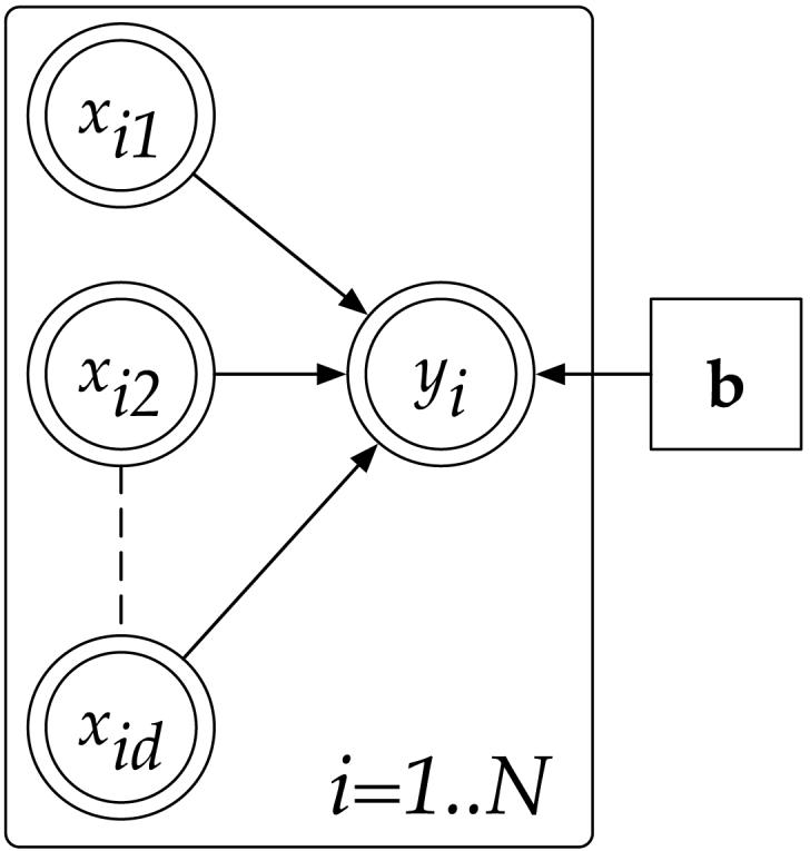
Graphical model for linear regression. Random variables are in circular nodes, observed random variables are in double circles, and point estimated parameters are in square nodes.

Figure 3.

Graphical model for Variational Bayesian Least Squares. Random variables are in circular nodes, observed random variables are in double circles, and point estimated parameters are in square nodes.

Figure 2.

Graphical model for Probabilistic Backfitting. Random variables are in circular nodes, observed random variables are in double circles, and point estimated parameters are in square nodes.

This new EM algorithm appears to only replace the matrix inversion in OLS by an iterative method, as others have done with alternative algorithms [13, 35]. However, the convergence guarantee of EM is an improvement over previous approaches. The true power of this probabilistic formulation becomes apparent when we add a Bayesian layer to achieve robustness in face of ill-conditioned data.

3.1 Automatic Feature Detection

From a Bayesian point of view, the parameters b_m should be treated probabilistically as well, such that we can integrate them out to safeguard against overfitting. For this purpose, as shown in Figure 3, we introduce precision variables α_m over each regression parameter b_m, as previously done in [39]:

$$\begin{array}{cc}\hfill p(\mathbf{b}\mid \alpha )& =\underset{m=1}{\overset{d}{\Pi }}{\left(\frac{{\alpha }_m}{2\pi }\right)}^{\frac{1}{2}}\exp \left(-\frac{{\alpha }_m}{2}{b}_m^2\right)\hfill \\ \hfill p\left(\alpha \right)& =\underset{m=1}{\overset{d}{\Pi }}\frac{b_{{\alpha }_m}^{a_{{\alpha }_m}}}{\mathrm{Gamma}\left(a_{{\alpha }_m}\right)}{\alpha }_m^{(a_{{\alpha }_m}-1)}\exp (-b_{{\alpha }_m}{\alpha }_m)\hfill \end{array}$$ (12)

where $\alpha \in {\mathfrak{R}}^{d\times 1}$ consists of α_m components. We now have a mechanism that infers the significance of each dimension's contribution to the observed output y. The key quantity that determines the relevance of a regression input is the parameter α_m. A priori, we assume that every b_m has a mean zero distribution with broad variance 1/α_m. If the posterior value of α_m turns out to be very large after all model parameters are estimated (equivalent to a very small variance of b_m), then the corresponding distribution of b_m must be sharply peaked at zero. Such a posterior gives strong evidence that b_m is very close to 0 and that the regression input x_m has no contribution to the output. Thus, this Bayesian model automatically detects irrelevant input dimensions and regularizes against ill-conditioned data sets.

Even though Eq. (12) looks very similar to that of [39] and later work of [3], our model has the key property that it is computationally efficient, requiring O(d) per EM iteration. In contrast, the methods of [3] and [39] take O(d³) per EM iteration and O(N³), respectively, becoming prohibitively expensive for large data sets with a very large input dimensionality, d. It is the fast, efficient nature of our proposed algorithm, Variational Bayesian Least Squares, that makes it suitable for real-time analysis of very large amounts of very high-dimensional data, as required in brain-machine interfaces. We discuss this application in more detail in the Evaluation section. The final model for VBLS has the following distributions:

$$\begin{array}{cc}\hfill y_i\mid {\mathbf{z}}_i& ~\text{Normal}(1^T{\mathbf{z}}_i,{\psi }_y)\hfill \\ \hfill z_{im}\mid b_m,{\alpha }_m,x_{im}& ~\text{Normal}\left(b_m{x}_{im},\frac{{\psi }_{zm}}{{\alpha }_m}\right)\hfill \\ \hfill b_m\mid {\alpha }_m& ~\text{Normal}\left(0,\frac{1}{{\alpha }_m}\right)\hfill \\ \hfill {\alpha }_m& ~\mathrm{Gamma}(a_{{\alpha }_m},b_{{\alpha }_m})\hfill \end{array}$$ (13)

As a note, it should be observed that the Gaussian prior used above for b_m is a standard prior in Bayesian linear regression, e.g., [3]. However, the Laplace prior could be used as well, and the result, when used with MAP estimation, will be similar to LASSO. We choose to not pursue this direction, but note that the Laplace density can be re-written in a hierarchical manner as done above by modeling the variance of b_m as a Gamma distribution with one hyperparameter, i.e., an exponential, as done by [9]. Integrating out the hyperparameter gives the Laplace marginal prior.

An EM-like algorithm [12] can be used to find the posterior updates of all distributions, where we maximize the incomplete log likelihood log p(y|X) by maximizing the expected complete log likelihood 〈log p(y,Z,b,α|X)〉:

$$\begin{array}{cc}\hfill \log p(\mathbf{y},\mathbf{Z},\mathbf{b},\alpha \mid \mathbf{X})& =\sum _{i=1}^N\log p(y_i\mid {\mathbf{z}}_i)+\sum _{i=1}^N\sum _{m=1}^d\log p(z_{im}\mid b_m,{\alpha }_m)+\sum _{m=1}^d\log p(b_m\mid {\alpha }_m)+\sum _{m=1}^d\log p\left({\alpha }_m\right)\hfill \\ \hfill & =-\frac{N}{2}\log {\psi }_y-\frac{1}{2{\psi }_y}\sum _{i=1}^N{(y_i-1^T{\mathbf{z}}_i)}^2-\frac{N}{2}\sum _{m=1}^d\log \frac{{\psi }_{zm}}{{\alpha }_m}-\sum _{m=1}^d\frac{{\alpha }_m}{2{\psi }_{zm}}{(z_{im}-b_m{x}_{im})}^2\hfill \\ \hfill & +\sum _{m=1}^d\log {\alpha }_m-\frac{1}{2}\sum _{m=1}^d{\alpha }_m{b}_m^2+\sum _{m=1}^d(a_{{\alpha }_m,0}-1)\log {\alpha }_m-\sum _{m=1}^d{b}_{{\alpha }_m,0}{\alpha }_m+\mathrm{const}\hfill \end{array}$$ (14)

where a_αm,0 and b_αm,0 are the initial parameter values that are set to reflect our confidence in the prior distribution of b_m. In order to obtain a tractable posterior distribution over all hidden variables b, z_i and α, we use a factorial variational approximation of the true posterior [12]: Q(α,b,Z)= Q(α,b)Q(Z). Note that the connection from the α_m to the corresponding z_im in Figure 3 is an intentional design. Under this graphical model, the marginal distribution of b_m becomes a Student t-distribution, allowing for traditional hypothesis testing [11]. The minimal factorization of the posterior into Q(α,b)Q(Z) would not be possible without this special design.

The variational Bayesian approximation used here allows us to reach a tractable posterior distribution over all hidden variables, such that we can proceed to infer the posterior distributions. Variational Bayesian learning approximates the intractable joint distribution over hidden states and parameters with a simpler distribution, e.g., assuming independence between hidden states and parameters such that the posterior distributions are factorized. An exact Bayesian solution is not feasible since one would need to compute the marginals of the joint posterior distribution—and this is not analytically possible. For discussions on the quality of variational Bayesian approximations and how they compare to the true solution, please refer to [1, 12, 17, 18]. We will return to this point in the Discussion section.

After some algebraic manipulations, the final EM posterior update equations become:E-step:

$${\Sigma }_z={\left(\frac{1}{{\psi }_y}{11}^T+{\Psi }_z^{-1}\langle \mathbf{A}\rangle \right)}^{-1}={\Psi }_z{\langle \mathbf{A}\rangle }^{-1}-\frac{{\Psi }_z{\langle \mathbf{A}\rangle }^{-1}{11}^T{\Psi }_z{\langle \mathbf{A}\rangle }^{-1}}{{\psi }_y+1^T{\Psi }_z{\langle \mathbf{A}\rangle }^{-1}1}$$ (15)

$$\begin{array}{cc}\hfill \langle {\mathbf{z}}_i\rangle & ={\Sigma }_z\left(\frac{1}{{\psi }_y}1y_i+{\Psi }_z^{-1}\langle \mathbf{A}\rangle \langle \mathbf{B}\mid \mathbf{A}\rangle {\mathbf{x}}_i\right)\hfill \\ \hfill & =\left(\frac{{\Psi }_z{\langle \mathbf{A}\rangle }^{-1}1}{{\psi }_y+1^T{\Psi }_z{\langle \mathbf{A}\rangle }^{-1}1}\right)y_i+\left(\langle \mathbf{B}\mid \mathbf{A}\rangle -\frac{{\Psi }_z{\langle \mathbf{A}\rangle }^{-1}{11}^T\langle \mathbf{B}\mid \mathbf{A}\rangle }{{\psi }_y+1^T{\Psi }_z{\langle \mathbf{A}\rangle }^{-1}1}\right){\mathbf{x}}_i\hfill \end{array}$$ (16)

$${\sigma }_{b_m\mid {\alpha }_m}^2=\frac{{\psi }_{zm}}{\langle {\alpha }_m\rangle }{\left(\sum _{i=1}^N{x}_{im}^2+{\psi }_{zm}\right)}^{-1}$$ (17)

$$\langle b_m\mid {\alpha }_m\rangle ={\left(\sum _{i=1}^N{x}_{im}^2+{\psi }_{zm}\right)}^{-1}\left(\sum _{i=1}^N\langle z_{im}\rangle x_{im}\right)$$ (18)

$${\widehat{a}}_{{\alpha }_m}=a_{{\alpha }_m,0}+\frac{N}{2}$$ (19)

$${\widehat{b}}_{{\alpha }_m}=b_{{\alpha }_m,0}+\frac{1}{2{\psi }_{zm}}\left\{\sum _{i=1}^N\langle z_{im}^2\rangle -{\left(\sum _{i=1}^N{x}_{im}^2+{\psi }_{zm}\right)}^{-1}{\left(\sum _{i=1}^N\langle z_{im}\rangle x_{im}\right)}^2\right\}$$ (20)

$$\langle {\alpha }_m\rangle =\frac{{\widehat{a}}_{\alpha m}}{{\widehat{b}}_{\alpha m}}$$ (21)

M-step:

$${\psi }_y=\frac{1}{N}\sum _{i=1}^N{(y_i-1^T\langle {\mathbf{z}}_i\rangle )}^2+1^T{\Sigma }_{z}1$$ (22)

$${\psi }_{zm}=\frac{1}{N}\sum _{i=1}^N\langle {\alpha }_m\rangle {(\langle z_{im}\rangle -\langle b_m\mid {\alpha }_m\rangle x_{im})}^2+\langle {\alpha }_m\rangle {\sigma }_{zm}^2+\langle {\alpha }_m\rangle {\sigma }_{b_m\mid {\alpha }_m}^2\left(\frac{1}{N}\sum _{i=1}^N{x}_{im}^2\right)$$ (23)

where 〈A〉, 〈B|A〉, ψ_z are diagonal matrices of 〈α〉, 〈b|α〉, ψ_z, respectively. Σ_z is a diagonal covariance matrix with a diagonal vector of ${\sigma }_z^2$. Note that $\langle z_{im}^2\rangle ={\langle z_{im}\rangle }^2+{\sigma }_{z_m}^2$, where ${\sigma }_{z_m}^2$ is the mth term of the vector ${\sigma }_z^2$.

The hyperparameters of α_m are learnt using EM, as shown by Eqs. (19) and (20). We set the initial values of the hyperparameters, a_α,0 and b_α,0, in an uninformative way and use values of $a_{{\alpha }_m},0={10}^{-8}$ and $b_{{\alpha }_m},0={10}^{-8}$ for all m = 1, … , d. This means that initial value of α_m is 1, with high uncertainty, i.e., α_m has a rather flat prior distribution.

Note that the update equation for 〈b_m|α_m〉 can be rewritten as:

$${\langle b_m\mid {\alpha }_m\rangle }^{\left(n+1\right)}=\left(\frac{\sum _{i=1}^N{x}_{im}^2}{\sum _{i=1}^N{x}_{im}^2+{\psi }_{zm}}\right){\langle b_m\mid {\alpha }_m\rangle }^{\left(n\right)}+\frac{{\psi }_{zm}}{s{\alpha }_m}\frac{\sum _{i=1}^N\left(y_i-{\langle \mathbf{b}\mid \alpha \rangle }^{\left(n\right)T}{\mathbf{x}}_i\right)x_{im}}{\sum _{i=1}^N{x}_{im}^2+{\psi }_{zm}}$$ (24)

Eq. (24) demonstrates that in the absence of a correlation between the current input dimension and the residual error, the first term causes the current regression coefficient to decay. The resulting regression solution regularizes over the number of retained inputs in the final regression vector, performing a functionality similar to Automatic Relevance Determination (ARD) [28]. The update equations of VBLS have an algorithmic complexity of O(d) per EM iteration, making it suitable for real-time analysis of large amounts of high-dimensional data— unlike previously proposed computationally prohibitive sparse linear regression methods that require O(d³) per EM iteration [3] or O(N³) [39]. One can further show that the marginal distribution of all b_m is a t-distribution with $t=\langle b_m\mid {\alpha }_m\rangle ∕{\sigma }_{b_m}\mid {\alpha }_m$ and $2{\widehat{a}}_{\alpha }$ degrees of freedom, which allows a principled way of determining whether a regression coefficient was excluded by means of standard hypothesis testing. Thus, Variational Bayesian Least Squares (VBLS) regression is a computationally efficient, full Bayesian treatment of the linear regression problem and is suitable for large amounts of high-dimensional data.

3.2 Pseudocode of Variational Bayesian Least Squares

The pseudocode for VBLS is listed below in Algorithm 1. To know when to stop iterating through the EM-based algorithm, we should monitor the incomplete log likelihood and stop when the value appears to have converged. However, since the calculation of the true posterior distribution Q(α,b,Z) is intractable, we cannot determine the true incomplete log likelihood. Hence, for the purpose of monitoring the incomplete log likelihood in the EM algorithm, we monitor a lower bound of the incomplete log likelihood instead. In the derivation of VBLS, we approximated Q(θ), where θ = {α,b,Z}, as Q(α, b)Q(Z). Using this variational approximation, we can derive the lower bound to the incomplete log likelihood (where φ= {ψ_y,ψ_z}) to be:

$$\begin{array}{cc}\hfill \log p(\mathbf{y}\mid \mathbf{X};\varphi )& \ge \int Q\left(\theta \right)\log \frac{p(\mathbf{y},\theta \mid \mathbf{X};\varphi )}{Q\left(\theta \right)}d\theta =\int Q\left(\theta \right)\log p(\mathbf{y},\theta \mid \mathbf{X};\varphi )d\theta -\int Q\left(\theta \right)\log Q\left(\theta \right)d\theta \hfill \\ \hfill & \ge {\langle \log p(\mathbf{y},\theta \mid \mathbf{X};\varphi \rangle }_{Q\left(\theta \right)}-\int Q\left(\theta \right)\log Q\left(\theta \right)d\theta \hfill \end{array}$$ (25)

where Eq. (25) simplifies to:

$$\begin{array}{cc}\hfill & \log p(\mathbf{y}\mid \mathbf{X};\varphi )\ge \hfill \\ \hfill & -\frac{N}{2}\log {\psi }_y-\frac{1}{2{\psi }_y}\sum _{i=1}^N(y_i^2-2y_i{1}^T\langle {\mathbf{z}}_i\rangle +1^T\langle {\mathbf{z}}_i{\mathbf{z}}_i^T\rangle 1)\hfill \\ \hfill & -\frac{N}{2}\sum _{m=1}^d\log {\psi }_{zm}-\sum _{m=1}^d\frac{\langle {\alpha }_m\rangle }{2{\psi }_{zm}}\sum _{i=1}^N(\langle z_{im}^2\rangle -2\langle z_{im}\rangle \langle b_m\mid {\alpha }_m\rangle x_{im}+\langle {(b_m\mid {\alpha }_m)}^2\rangle x_{im}^2)\hfill \\ \hfill & -\frac{1}{2}\sum _{m=1}^d\langle {\alpha }_m\rangle \langle {(b_m\mid {\alpha }_m)}^2\rangle -\frac{N-1}{2}\sum _{m=1}^d\log {\widehat{b}}_{{\alpha }_m}-{\widehat{a}}_{{\alpha }_m}\hfill \\ \hfill & -\frac{1}{2}\log \mid {\Sigma }_z^{-1}\mid -\sum _{m=1}^d\log {\widehat{b}}_{{\alpha }_m}+\frac{1}{2}\sum _{m=1}^d\langle {\alpha }_m\rangle ({\sigma }_{b_m\mid {\alpha }_m}^2+1)+\mathrm{const}\hfill \end{array}$$ (26)

We stop iterating when the lower bound to the incomplete log likelihood has converged (i.e., when a certain likelihood tolerance, t, has been reached). Additionally, note that the input and output data are assumed to be centered (i.e. have a mean of 0) before we analyze the data set with VBLS.

Algorithm 1 Pseudocode for VBLS.

0: Initialization: a_α,0 = 10⁻⁸1, b_α,0 = 10⁻⁸1; threshold value for lower bound to the incomplete log likelihood, t = 10⁻⁶

1: Start EM iterations:

2: repeat

3: Perform the E-step: Calculate Eqs. (15) to (20)

4: Perform the M-step: Calculate Eqs. (22) and (23)

5: Monitor the lower bound to the incomplete log likelihood, Eq. (26), to see if the likelihood tolerance t has been reached

6: until convergence of Eq. (26)

4 Evaluation

We now turn to the application and evaluation of VBLS in the context of predicting EMG data from neural data recorded in primary motor (M1) and premotor (PM) cortices of monkeys. The key questions addressed in this application were i) whether EMG data can be reconstructed accurately with good generalization, ii) how many neurons contribute to the reconstruction of each muscle, and iii) how well the VBLS algorithm compares to other analysis techniques. The underlying assumption of this analysis was that the relationship between cortical neural firing and muscle activity is approximately linear.

Before applying VBLS to real data, however, we first run it on synthetic data sets where “ground truth” is known, in order to better evaluate its performance in a controlled setting.

4.1 Synthetic Data

4.1.1 Data sets

We generated random input training data consisting of 100 dimensions, 10 of which were relevant dimensions. The other 90 were either irrelevant or redundant dimensions, as we explain below. Each of the first 10 input dimensions was drawn from a Gaussian distribution with some random covariance. The output data was then generated from the relevant input data using the vector $\mathbf{b}\in {\mathfrak{R}}^{10\times 1}$, where each coefficient of b, b_m, was drawn from a Normal(0, 100) distribution, subject to the fact that it cannot be zero (since this would indicate an irrelevant dimension). Additive mean-zero Gaussian noise of varying levels was added to the outputs.

Noise in the outputs was parameterized with the coefficient of determination, r², of standard linear regression, defined as:

$$r^2=\frac{({\sigma }_y^2-{\sigma }_{res}^2)}{{\sigma }_y^2}$$

where ${\sigma }_y^2$ is the variance of the outputs and ${\sigma }_{res}^2$ is the variance of the residual error. We added noise scaled to the variance of the noiseless outputs $\stackrel{‒}{y}$ such that ${\sigma }_{noise}^2=c{\sigma }_{\stackrel{‒}{y}}^2$, where $c=\frac{1}{r^2}-1$. Results are quantified as normalized mean squared errors (nMSE), that is, the mean squared error on the test set normalized by the variance of the outputs of the test set. Note that the best normalized mean squared training error that can be achieved by the learning system under this noise level is 1 − r², unless the system overfits the data. We used a value of r² = 0.8 for high output noise and a value of r² = 0.9 for lower output noise.

A varying number of redundant data vectors was added to the input data, generated from random convex combinations of the 10 relevant vectors. Finally, we added irrelevant data columns, drawn from a Normal(0,1) distribution, until a total of 100 input dimensions was reached, generating training input data that contained irrelevant and redundant dimensions.

We created the test data set in a similar manner except that the input data and output data were left noise-free. For our experiments, we considered a synthetic training data set with N = 1000 data samples and a synthetic test data set with 20 data samples. We examined the following four different combinations of redundant, v, and irrelevant, u, input dimensions in order to better analyze the performance of the algorithms on different data sets:

1. v = 0, u = 90 (all the 90 input dimensions are irrelevant)

2. v = 30, u = 60

3. v = 60, u = 30

4. v = 90, u = 0 (all the 90 input dimensions are redundant)

4.1.2 Methods

We compared VBLS to four other methods that were previously described in Section 2: i) ridge regression, ii) stepwise regression, iii) PLS regression and iv) LASSO regression. For ridge regression, we introduced a small ridge parameter value of 10⁻¹⁰ to avoid ill-conditioned matrix inversions. We used Matlab's “stepwisefit” function to run stepwise regression. The number of PLS projections for each data set fit was found by leave-one-out cross-validation. Finally, we chose the optimal tuning parameter in LASSO regression using k-fold cross-validation.

4.1.3 Results

For evaluation, we calculated the prediction error on noiseless test data, using the learned regression coefficients from each technique. Results are quantified as normalized mean squared errors (nMSE). Figure 4 shows the average prediction error for noiseless test data, given training data where the output noise is either low (r² = 0.9) or high (r² = 0.8).

Figure 4.

Average normalized mean squared prediction error for synthetic 100 input-dimensional data with an varying levels of output noise in the training data, averaged over 10 trials. There are 10 relevant input dimensions and a total of 90 redundant and irrelevant input dimensions. The number of redundant dimension is denoted by v, and the number of irrelevant dimensions is u.

All the algorithms were executed on 10 randomly generated sets of data. The predictive nMSE results reported in Figure 4 were averaged over the 10 trials. Note that the best training nMSE values possible under the two noise conditions are 0.1 for the low noise case and 0.2 for the high noise case. The training nMSE values were omitted for both graphs, since all algorithms attained training errors that were around the lowest possible values.

From Figures 4(a) and 4(b), we see that regardless of output noise level, VBLS achieves either the lowest predictive nMSE value or a predictive nMSE value comparable to that of the other four algorithms. In general, as the number of redundant input dimensions increases and the number of irrelevant input dimensions decreases, the prediction error improves (i.e., it decreases). This may be attributed to the fact that redundancy in the input data provides more “information”, making the problem easier to solve.

The performance of stepwise regression degrades as the number of redundant dimensions increases, as shown in Figures 4(a) and 4(a), due to its inability to cope with collinear data. LASSO regression appears to perform quite well, compared to PLS regression and ridge regression. This is unsurprising, given it is known for its ability to produce sparse solutions.

In summary, we can confirm that VBLS performs very well—as well as or better than classical robust regression methods (such as LASSO) on synthetic tests. Interestingly, PLS regression and ridge regression are significantly inferior in problems that have a large number of irrelevant dimensions. Stepwise regression has deteriorated performance as soon as co-linear inputs are introduced.

4.1.4 Non-Normal Synthetic Data

We can also examine synthetic data sets which do not correspond to the generative model (i.e., data and noise that are not generated from Normal distributions) in order to evaluate how dependent our model is on the Normal prior distributions that we assumed.

The synthetic data is generated in a similar fashion as in Section 4.1.1, with 100 dimensions—10 of which are relevant dimensions. The other 90 dimensions are chosen to be either irrelevant or redundant. The first 10 relevant input dimensions were generated from a multi-modal distribution, instead of a Normal distribution. Specifically, each of the relevant 10 input dimensions was drawn from a sum/mixture of 10 Gaussian distributions, with each Gaussian distribution having a different mean and variance, i.e., $x_m~{\sum }_{p=1}^N$ Normal $({\mu }_p,{\sigma }_p^2)$, for m = 1, …, 10 where σ_p is drawn randomly from a uniform distribution between 0 and 2 and µ_p is drawn similarly from a uniform distribution between 0 and 2. The second difference between this non-Normal synthetic data set and the data set used in Section 4.1.1 is the additive output noise. Instead of Gaussian distributed noise, noise drawn from a Student t-distribution was added to the outputs. We chose a noise level of r² = 0.9999 for the output noise, such that the noise was scaled to the variance of the noiseless outputs $\stackrel{‒}{y}$. Redundant and irrelevant data vectors were added to the input data in a similar way as described in Section 4.1.1. The test data was created in a similar manner, except the input and output data were left noise-free. As in Section 4.1.1, we considered synthetic training data with N = 1000 data samples and a synthetic test data set with 20 data samples.

Figure 5 shows the prediction nMSE values, averaged over 10 trials. We can observe that both VBLS and LASSO outperform the other classical regression methods on non-Normal synthetic data sets. This figure demonstrates that even for data sets that do not follow the Normal prior distributions assumed in our generative model, VBLS continues to perform quite competitively.

Figure 5.

Average normalized mean squared prediction error for synthetic non-Normal 100 input-dimensional data with an output noise of r² = 0.9999 in the training data, averaged over 10 trials. There are 10 relevant input dimensions and a total of 90 redundant and irrelevant input dimensions. The number of redundant dimension is denoted by v, and the number of irrelevant dimensions is u. Each relevant dimension of the training data is drawn from a multi-modal distribution (a mixture of Gaussian distributions), and the output noise is drawn from a Student t-distribution.

4.2 EMG Prediction from Neural Firing

4.2.1 Data sets

We investigated data from two different neurophysiological experiments. In the first experiment by Sergio & Kalaska [34], a monkey moved a manipulandum in a center-out task in eight different directions, equally spaced in a horizontal planar circle of 8cm radius. A variation of this experiment held the manipulandum rigidly in place, while the monkey applied isometric forces in the same eight directions. In both conditions (whether the monkey was applying a movement or an isometric force), feedback was given through visual display on a monitor. Neural activity for 71 M1 neurons was recorded in all conditions, along with the EMG outputs of 11 muscles¹. After preprocessing, we obtained a total of 2320 data samples for each neuron/muscle pair, collected over all eight directions and for both movement and isometric force conditions. Each data sample consisted of the average firing rates from a particular neuron (averaged over a window of 10msec) and the corresponding EMG activation² from a particular muscle. A sampling interval of 10msec was used. For each sample in this data set, a delay of 50msec between M1 cortical neural firing and EMG muscle activation was empirically chosen, based on estimates from measurements.

The second experiment, conducted by Kakei et al. [19, 20], involved a monkey trained to perform eight different combinations of wrist flexion-extension and radial-ulnar movements while in three different arm postures (pronated, supinated and midway between the two). These experiments resulted in two data sets. For the first, the EMG outputs of 7 contributing muscles³ were recorded, along with the neural data of 92 M1 neurons at all three wrist postures, resulting in 2616 data samples for each neuron/muscle pair. As for the Sergio & Kalaska data set, each data sample consisted of the average firing rates from a particular neuron (averaged over a window of 10msec) and the corresponding EMG activation from a particular muscle. A sampling interval of 10msec was used. For each sample in this data set, a delay of 20msec⁴ between M1 cortical neural firing and EMG muscle activation was chosen empirically, based on estimates from measurements. The second data set also included EMG outputs of the same 7 muscles, but, this time, contained the recorded spiking data of 72 PM neurons at the three wrist postures. After preprocessing, this second data set had 2592 data samples for each neuron/muscle pair. For each sample, a delay of 30msec⁵ between PM cortical neural firing and EMG muscle activation was assumed.

4.2.2 Methods

As a baseline comparison, EMG reconstruction was obtained through a combinatorial search over possible regression models. This approach served as our baseline study (referred to as ModelSearch in the figures). A particular model is characterized by a subset of neurons that is used to predict the EMG data. For the Sergio & Kalaska data, given 71 neurons, the number of possible models that exist for a particular muscle is:

$$\sum _{m=1}^{71}\left(\begin{array}{c}\hfill 71\hfill \\ \hfill m\hfill \end{array}\right)$$

Since the order of the contributing neurons is not important, the above expression lists the combinations instead of permutations of neurons. This value is too large for an exhaustive search. Therefore, we considered only possible combinations of up to 20 neurons, which required several weeks of computation on a 30-node cluster computer. The optimal predictive subset of neurons was determined from a series of 8-fold cross-validation sets.

For both data sets, the cross-validation procedure used in the baseline study was used in order to determine the optimal subset of neurons. Cross-validation was done in the context of the behavioral experiments and not in a statistically randomized way. For the Sergio & Kalaska experiment, the data was separated into different force categories (isometric force versus force generated during movement) and movement directions in space. Thus, cross-validation asked the meaningful question of whether isometric and movement conditions are predictive of each other and whether there is spatial generalization. Similarly, for the Kakei et al. experiment, data was separated into directional movements at the wrist (supinated, pronated and midway between the two wrist movements) and directional movements in space, which again allowed cross-validation to make meaningful statements about generalization over postures and space.

Figure 6 shows how these 8 cross-validation sets are constructed from the Sergio & Kalaska data. This baseline study (i.e., ModelSearch) served as a comparison for ridge regression, stepwise regression, PLS regression, LASSO regression and VBLS. These five algorithms used the same validation sets employed in the baseline study. Again, as described in Section 4.1.2, ridge regression was implemented using a small ridge regression parameter of 10⁻¹⁰, in order to avoid ill-conditioned matrices. We used Matlab's “stepwisefit” to run stepwise regression, and the number of PLS projections for each data fit was found by leave-one-out cross-validation. The average normalized mean squared error values depicted in Figure 9(a) demonstrate how well each algorithm performs, averaging the generalization performances over all the cross-validation sets from Figure 6.

Figure 6.

Details of how the 8 cross-validation sets are created from the Sergio & Kalaska M1 neural data set. For each type of force applied by the monkey to the manipulandum, there are 8 possible directions that the manipulandum could have been moved. Each circle shown above is partitioned into 8 equal portions, corresponding to the 8 directional movements and numbered in increasing order (clockwise) starting from 1.

Figure 9.

Normalized mean squared error for M1 neurons, averaged over all cross-validation sets and over all muscles. Figure 6 shows the 8 cross-validation sets used in the Sergio & Kalaska (1998) M1 neural data set, and Figure 7 shows the 6 cross-validation sets used for the Kakei et al. (1999) M1 neural data set.

The average number of relevant neurons⁶ (i.e., not including irrelevant neurons and neurons providing redundant information), shown in Figure 11(a), was calculated by averaging over the number of relevant neurons in each of the 8 training sets in Figure 6.

Figure 11.

Average number of relevant M1 neurons found over all the 8 cross-validation sets from Figure 6 (for Sergio & Kalaska data) and over all the 6 cross-validation sets from Figure 7 (for Kakei et al. data). Results are shown for each muscle in each data set.

The final set of relevant neurons, used in Figure 13(a) to calculate the percentage match of relevant neurons relative to those found by the baseline study (ModelSearch), was reached for each algorithm (except VBLS) by taking the common neurons found to be relevant over the 8 cross-validation sets. The relevant neurons found by VBLS and reported in Figure 13(a) were obtained by using the entire data set, since no cross-validation procedure is required by VBLS (i.e., dividing the data into separate training and test sets is not necessary). As with all Bayesian methods, VBLS performs more accurately as the data size increases, without the danger of overfitting. Inference of relevant neurons in PLS was based on the subspace spanned by the PLS projections, while relevant neurons in VBLS were inferred from t-tests on the regression parameters, using a significance of p < 0.05. Stepwise regression determined the number of relevant neurons from the inputs that were included in the final model. Note that since ridge regression retained all input dimensions, this algorithm was omitted in relevant neuron comparisons.

Figure 13.

Percentage of M1 neuron matches found by each algorithm, as compared to those found by the baseline study (ModelSearch), shown for each muscle in the Sergio & Kalaska data set and Kakei et al. data set.

Analogous to the first data set, a combinatorial analysis was performed on the Kakei et al. M1 neural and PM neural data sets in order to determine the optimal set of M1 and PM neurons contributing to each muscle (i.e. producing the lowest possible prediction error) in a series of 6-fold cross-validation sets. Figures 7 and 8 show the 6 cross-validation sets used for the M1 and PM neural data sets. PLS, stepwise regression, ridge regression and VBLS were applied using the same cross-validation sets, employing the same procedure described for the Sergio & Kalaska data set. The average normalized mean squared error values shown in Figures 9(b) and 10 illustrate the generalization performance of each algorithm, averaged over all the cross-validation sets shown in Figures 7 and 8⁷. The average number of relevant neurons shown in Figures 11(b) and 12 was calculated by averaging over the number of relevant neurons found in each of the 6 training sets from Figures 7 and 8. As for the Sergio & Kalaska data set, the final set of relevant neurons, used in Figures 11(b) and 12, was obtained for each algorithm (except VBLS) by taking the common neurons found to be relevant over the 6 cross-validation sets.

Figure 7.

Details of how the 6 cross-validation sets are created from the Kakei et al. M1 neural data set. For each of the three wrist positions, there are 8 possible directional movements. Each circle shown above is partitioned into 8 equal sections, corresponding to the 8 directional movements and numbered in increasing order (clockwise) starting from 1.

Figure 8.

Details of how the 6 cross-validation sets are created from the Kakei et al. PM neural data set. For each of the three wrist positions, there are 8 possible directional movements. Each circle shown above is partitioned into 8 equal sections, corresponding to the 8 directional movements and numbered in increasing order (clockwise) starting from 1.

Figure 10.

Average normalized mean squared error for PM neurons, averaged over all 6 cross-validation sets shown from Figure 8 and over all muscles. Results are shown for the Kakei et al. (1999) PM neural data set.

Figure 12.

Average number of relevant PM neurons found over the 6-fold cross-validation sets from Figure 8 for Kakei et al. data. Results are shown for each muscle.

4.2.3 Results

Figures 9 and 10 show that VBLS resulted in a generalization error comparable to that produced by ModelSearch (i.e., the baseline study). In the Kakei et al. M1 and PM neural datasets, all algorithms performed similarly, as we see on the right hand side of Figures 9(b) and 10. However, ridge regression, stepwise regression, PLS regression and LASSO regression performed far worse on the Sergio & Kalaska M1 neural dataset, with ridge regression attaining the worst error, as we see on the right hand side of Figure 9(a). Such performance is typical for traditional linear regression methods on ill-conditioned high-dimensional data, motivating the development of VBLS.

Interestingly, in Figure 9(b), we observe that the prediction errors of ridge regression and of the baseline study (i.e. ridge regression using a selected subset of M1 neurons) are quite similar for the Kakei et al. M1 neural data set. This suggests that, for this particular data set, there is little advantage in performing a time-consuming manual search for the optimal subset of neurons. A similar observation can be made for the Kakei et al. PM neural data set when examining Figure 10, although this effect is less pronounced in the PM neural data set. In contrast, Figure 9(a) shows a sharp difference between the predictive error values of ridge regression and the baseline study's combinatorial-like model search. This may be attributed to the fact that the Sergio & Kalaska M1 neural data set is somehow much richer and hence, more challenging to analyze.

The average number of relevant M1 neurons found by VBLS was slightly higher than the baseline study, as seen in Figure 11. This is unsurprising, since the baseline studies did not consider all possible combination of neurons. For example, the baseline study for the Sergio & Kalaska data set considered possible combinations of up to only 20 neurons, instead of the full set of 71 neurons. In particular, notice that in Figures 11(b) and 12, small amounts of the total 92 M1 neurons and 72 PM neurons were found to be relevant by the baseline study for certain muscles (e.g., muscles 1, 6 and 7).

We compared the relevant neurons identified by each algorithm with those found by the baseline combinatorial-like model search in an attempt to evaluate how well each algorithm performed in comparison to the model search approach. Table 1 shows the percentage of neuron matches found by each algorithm, averaged over all the muscles of the data set. The percentage of neuron matches was calculated by considering the list of relevant neurons found by the baseline study. The number of neurons in this list that the algorithm was successfully at identifying as relevant was counted, and the percentage of relevant neuron matches was calculated using this value.

Table 1.

Percentage of neuron matches found by each algorithm, as compared to those found by the baseline study (ModelSearch), averaged over all muscles in each data set. The percentage of relevant neuron matches for an algorithm is calculated by considering the list of relevant neurons found by the baseline study. The number of neurons in this list that the algorithm was successfully at identifying as relevant was counted, and the percentage of neuron matches calculated using this value.

	STEP	PLS	LASSO	VBLS
Sergio & Kalaska (1998) M1 neural data set	7.2 %	7.4 %	6.4 %	94.2 %
Kakei et al. (1999) M1 neural data set	65.1 %	42.9 %	80.6 %	94.4 %
Kakei et al. (1999) PM neural data set	22.9 %	14.2 %	44.5 %	91.5 %

Table 1 shows that the relevant neurons identified by VBLS coincided at a very high percentage with those of the baseline model, while stepwise and PLS regression had inferior outcomes. This table illustrates that VBLS was able to reproduce comparable results to a combinatorial like model search approach. However, the main advantage of VBLS arises in its speed: VBLS took 8 hours for all validation sets on a standard PC while the model search took weeks on a cluster computer. LASSO regression matched a high percentage of the relevant M1 and PM neurons in the Kakei et al. data set, but fared far worse on the Sergio & Kalaska data set. These percentage values for the Kakei et al. data sets are perhaps inflated and should be given less consideration, since the numbers of relevant M1 and PM neurons found by the baseline study are relatively small for certain muscles. Figures 13(a), 13(b) and 14 show the detailed breakdown of percentage M1 and PM neuron matches for each algorithm on each muscle. The consistent and good generalization properties of VBLS on all neural data sets, as shown in Figures 9(a), 9(b) and 10, suggests that the Bayesian approach of VBLS suffciently regularizes the participating neurons such that no overfitting occurs, despite finding a larger number of relevant neurons.

Figure 14.

Percentage of PM relevant neuron matches found by each algorithm, as compared to those found by the baseline study (ModelSearch), shown for each muscle in the Kakei et al. data set.

One could argue that the results of Table 1 are not so meaningful, given that VBLS finds a large number of relevant neurons. However, we should add that LASSO regression also finds a high number of relevant neurons, especially for the Kakei M1 and PM neural datasets, as shown in Figures 11(b) and 12. In some cases (for the PM neural data set), LASSO regression finds more relevant neurons than VBLS. Regardless, the percentage match found by LASSO was lower than that found by VBLS (80.6% and 44.5% on the Kakei M1 and PM data sets for LASSO compared to 94.4% and 91.5% for VBLS). The percentage match criterion seems to be have high correlation with the quality of generalization of each of the algorithms.

In general, VBLS achieved comparable performance with the baseline study when reconstructing EMG data from M1 or PM neurons. Note that VBLS is an iterative statistical method, which performs slower than classical “one-shot“ linear least squares methods (i.e., on the order of several minutes for the data sets in our analyses). Nevertheless, it achieves comparable results with our combinatorial model search, while performing at much faster speeds.

4.3 Real-time Analysis for Brain-Machine Interfaces

Due to its computationally efficient nature, the VBLS algorithm presented in Algorithm 1 lends itself to scenarios where fast, online learning with large amounts of high-dimensional data is required, such as real-time brain-machine interfaces. Previous work by [31, 32] has shown that an online version of the Variational Bayes framework can be derived, such that online model selection can be done with guaranteed convergence. A scalar discount factor or forgetting rate is typically introduced in order to forget estimates that were calculated earlier (and hence, were less accurate). [31, 32] introduce a time-dependent schedule for the discount factor and prove convergence of the online EM-based algorithm. Since the main focus of this manuscript is on the batch form of the algorithm, we will show only a proof-of-concept and use a constant-valued discount factor in order to demonstrate that the batch VBLS algorithm can be translated into incremental form. We leave the detailed theoretical development of the online version of the algorithm with a discount factor schedule for another paper.

In particular, we introduce a forgetting rate, 0 ≤ λ ≤ 1, to exponentially discount data collected in the past, as done in [23]. The forgetting rate enters the algorithm by accumulating sufficient statistics of the batch algorithm in an incremental way. We can then extract the sufficient statistics by examining the batch EM equations, Eqs. (15) to (23). The incremental EM update equations for the kth time step, when data sample {x_k, y_k} is available, are then:E-step:

$$s_k={\left({\psi }_y\right)}_{k-1}+1^T{\left({\Psi }_z\right)}_{k-1}{\langle \mathbf{A}\rangle }_{k-1}^{-1}1$$ (27)

$${\left({\Sigma }_z\right)}_k={\left({\Psi }_z\right)}_{k-1}{\langle \mathbf{A}\rangle }_{k-1}^{-1}-\frac{{\left({\Psi }_z\right)}_{k-1}{\langle \mathbf{A}\rangle }_{k-1}^{-1}{11}^T{\left({\Psi }_z\right)}_{k-1}{\langle \mathbf{A}\rangle }_{k-1}^{-1}}{s_k}$$ (28)

$$\langle {\mathbf{z}}_k\rangle =\left(\frac{{\left({\Psi }_z\right)}_{k-1}{\langle \mathbf{A}\rangle }_{k-1}^{-1}1}{s_k}\right)y_k+{\langle \mathbf{B}\rangle }_{k-1}{\mathrm{x}}_k-\frac{{\left({\Psi }_z\right)}_{k-1}{\langle \mathbf{A}\rangle }_{k-1}^{-1}{11}^T{\langle \mathbf{B}\rangle }_{k-1}}{s_k}{\mathbf{x}}_k$$ (29)

$${\left({\sigma }_{b_m}^2\right)}_k=\frac{{\left({\psi }_{zm}\right)}_{k-1}}{{\langle {\alpha }_m\rangle }_{k-1}}({\Sigma }_k^{x^2}+{\left({\psi }_{zm}\right)}_{k-1}{)}^{-1}$$ (30)

$${\langle b_m\rangle }_k=\left(\frac{{\Sigma }_k^{x^2}}{{\Sigma }_k^{x^2}+{\left({\psi }_{zm}\right)}_{k-1}}\right){\langle b_m\rangle }_{k-1}+\frac{{\left({\psi }_{zm}\right)}_{k-1}}{{\langle {\alpha }_m\rangle }_{k-1}}\frac{\left({\Sigma }_k^{yx}-{\Sigma }_k^{x{x}^T}{\langle \mathbf{b}\rangle }_{k-1}\right)}{\left({\Sigma }_k^{x^2}+{\left({\psi }_{zm}\right)}_{k-1}\right)s_k}$$ (31)

$${\left({\widehat{a}}_{\alpha }\right)}_k=a_{\alpha 0}+\frac{{\Sigma }_k^N}{2}$$ (32)

$${\left({\widehat{b}}_{\alpha }\right)}_k=b_{\alpha m0}+\frac{1}{2{\left({\psi }_{zm}\right)}_{k-1}}\left\{{\Sigma }_k^N{\left({\Sigma }_z\right)}_k+{\Sigma }_k^{\langle z^2\rangle }-{\left({\Sigma }_k^{x^2}+{\left({\psi }_{zm}\right)}_{k-1}\right)}^{-1}{\left({\Sigma }_k^{\langle z\rangle x}\right)}^2\right\}$$ (33)

$${\langle {\alpha }_m\rangle }_k=\frac{{\left({\widehat{a}}_{\alpha }\right)}_k}{{\left({\widehat{b}}_{\alpha m}\right)}_k}$$ (34)

M-step:

$${\left({\psi }_y\right)}_k=\frac{1}{{\Sigma }_k^N}{\left(1-\frac{{\left({\Psi }_z\right)}_{k-1}{\langle \mathbf{A}\rangle }_k^{-1}1}{s_k}\right)}^2\left({\Sigma }_k^{y^2}-2{\langle \mathbf{b}\rangle }_{k-1}^T{\Sigma }_k^{yx}+{\langle \mathbf{b}\rangle }_{k-1}^T{\Sigma }_k^{x{x}^T}{\langle \mathbf{b}\rangle }_{k-1}\right)+1^T{\left({\Sigma }_z\right)}_{k}1$$ (35)

$${\left({\psi }_{zm}\right)}_k=\frac{{\left({\psi }_{zm}\right)}_{k-1}^2}{{\langle {\alpha }_m\rangle }_k{s}_k^2}\frac{\left({\Sigma }_k^{y^2}-2{\langle \mathbf{b}\rangle }_k^T{\Sigma }_k^{yx}+{\langle \mathbf{b}\rangle }_k^T{\Sigma }_k^{x{x}^T}{\langle \mathbf{b}\rangle }_k\right)}{{\Sigma }_k^N}+{\langle {\alpha }_m\rangle }_k{\left({\sigma }_{b_m}^2\right)}_k\frac{{\Sigma }_k^{x^2}}{{\Sigma }_k^N}+{\langle {\alpha }_m\rangle }_k{\Sigma }_z$$ (36)

where (Σ_z)_k is Σ_z at time step k (and similarly, for all the other parameter values) and the sufficient statistics are:

$$\begin{array}{cc}\hfill {\Sigma }_k^{x^2}& ={\Sigma }_{k-1}^{x^2}+x_{im}^2\hfill \\ \hfill {\Sigma }_k^{y^2}& ={\Sigma }_{k-1}^{y^2}+y_i^2\hfill \\ \hfill {\Sigma }_k^{yx}& ={\Sigma }_{k-1}^{yx}+y_i{x}_{im}\hfill \\ \hfill {\Sigma }_k^{x{x}^T}& ={\Sigma }_{k-1}^{x{x}^T}+{\mathbf{x}}_i{\mathbf{x}}_i^T\hfill \\ \hfill {\Sigma }_k^N& =\lambda {\Sigma }_{k-1}^N+1\hfill \\ \hfill {\Sigma }_k^{\langle z\rangle x}& =\lambda {\Sigma }_{k-1}^{\langle z\rangle x}+\langle z_{im}\rangle x_{im}\hfill \\ \hfill {\Sigma }_k^{\langle z^2\rangle }& =\lambda {\Sigma }_{k-1}^{\langle z^2\rangle }+{\langle z_{im}\rangle }^2\hfill \end{array}$$

with certain sufficient statistics discounted by λ, as necessary.

Note that both neural data sets are inherently real-time data-collected online, stored, and then analyzed in batch form (i.e., a sampling interval is used and a delay between neural firing and EMG activity is empirically chosen in order to extract the data samples to be used in the batch form of the data). As a result, in the real-time simulations, we took the batch form of the data and presented it sequentially, one data sample at each time step.

We applied the real-time version of VBLS on the Sergio & Kalaska data set, since this was the more interesting of the three presented in Section 4.2.1. We used a forgetting rate of λ = 0.999, assumed each sample of the data set arrived sequentially at different time steps, and iterated through the incremental VBLS equations (27) to (36) twice for each time step.

Figure 15(a) shows the coefficient of determination values, r² (where r² = 1 − nMSE), for both the batch and real-time versions of VBLS on the entire Sergio & Kalaska data set. Figure 15(b) shows the number of relevant M1 neurons found by batch VBLS and real-time VBLS for the same data set. For the real-time version of VBLS, the r² values and relevant neurons reported were from the last time step. We can see from both figures that the real-time and batch versions of VBLS achieve a similar level of performance. The average r² values (averaged over all 11 muscles) confirm this: batch VBLS had an average r² value of 0.7998, while real-time VBLS had an average r² value of 0.7966.

Figure 15.

Coefficient of determination values, r² = 1−nMSE, and number of relevant neurons found by VBLS—both the batch and real-time versions. For the real-time, incremental version of VBLS, the relevant neurons found in the last time step is shown.

4.4 Interpretation of Analysis of Neural Data

While the main focus of this paper lies in the introduction of a robust linear regression technique for high-dimensional data, we would like to discuss how our analysis technique can be exploited for the interpretation of the neurophysiological data that we used in this study.

In Sergio & Kalaska [34], one of the main results was that the firing of the reported M1 neurons had strong correlation with EMG-like (or force-like) signals in both movement and isometric conditions. In contrast, evidence for correlations with kinematic data (such as movement direction, velocity, or target direction) was less pronounced. Figures 16 and 17 reproduce similar illustrations to Figures 3A and 3B in [34]. The two figures show the EMG activity of the infraspinatus muscle in all eight isometric force production directions (Figure 16) and movement directions (Figure 17). The trajectories, shown in (x, y) coordinates, taken by the hand are illustrated in the center of each figure. These center figures are taken from the original figures of [34], since we did not have access to the hand trajectory data. Each of the eight EMG plots in Figures 16 and 17 shows the following three EMG traces: i) the raw average EMG trajectories; ii) the predicted EMG activity from M1 neurons, as obtained by VBLS using all available data in all conditions; and iii) a cross-validation fit that was obtained by VBLS using only half of the data: for the isometric condition, only movement data was used for fitting, and for the movement condition, only isometric data was used for fitting. This last cross-validated fit tests how well isometric M1 neural recordings can predict movement EMG and how well movement-related M1 neural recordings can predict isometric EMG. Alternatively, it tests whether the neuron to EMG relationship is the same between the isometric and the movement conditions.

Figure 16.

Observed vs. predicted EMG traces under isometric force conditions for the infraspinatus muscle, from the Sergio & Kalaska data set. The center plot shows the trajectories in eight different directions (in the (x, y) plane) taken by the hand. This figure is taken from Sergio & Kalaska. Each of the eight plots surrounding this center plot shows EMG traces over time for each hand trajectory, illustrating the following: i) the observed averaged EMG activity, ii) the predicted EMG activity, as obtained by VBLS using the entire data set (VBLS-full), and iii) the predicted EMG activity, as obtained VBLS using only movement data for fitting (VBLS-cv).

Figure 17.

Observed vs. predicted EMG traces under movement force conditions for the infraspinatus muscle, from the Sergio & Kalaska M1 data set. The center plot shows the trajectories in eight different directions (in the (x, y) plane) taken by the hand. This figure is taken from Sergio & Kalaska. Each of the eight plots surrounding this center plot shows the EMG traces over time for each hand trajectory, illustrating the following: i) the observed averaged EMG activity, ii) the predicted EMG activity, as obtained by VBLS using the entire data set (VBLS-full), and iii) the predicted EMG activity, as obtained VBLS using only isometric data for fitting (VBLS-cv).

As Figures 16 and 17 both show, M1 neural firing predicts the EMG traces very well in general. The cross-validation tests also demonstrate very good EMG reconstruction, thus confirming Sergio & Kalaska's results [34] that the recorded M1 neurons have sufficient information to extract signals of the time-varying dynamics and the temporal envelopes of EMG activities.

The main message in Kakei et al. [19, 20] was that one can find neurons in M1 that carry intrinsic (muscle-based) and neurons that carry extrinsic ((x, y) task space) information. In contrast, PM had predominantly extrinsic neurons. For our data analysis, we had access to the average firing rates of the M1 and PM neurons and the corresponding EMG traces, as well as the (x, y) movement as performed by the hand. Thus, we used VBLS to predict the EMG activity in all three arm posture conditions (pronated, supinated and midway between the two) from the neural firing and to predict the (x, y)-velocity trajectories from neural firing. Note that all this data was obtained from the same highly trained monkey, such that it was possible to i) re-use EMG data obtained during the M1 experiment as target for the PM data and ii) share the same (x, y) data across the M1 and PM experiment. We illustrate our results in a similar form as in Figures 16 and 17, showing plots for the extensor carpi radialis brevis (ECRB) muscle and only for the supination posture. Figure 18(b) shows the EMG fits for M1 neurons, while Figure 19(b) shows the same fits for PM neurons. The center plots illustrate recorded (x, y) movement in the horizontal plane in this posture. Interestingly, both M1 and PM neurons achieve a very good EMG reconstruction⁸. Figures 20(b), 22(b), 21(b) and 23(b) demonstrate the (x, y)-velocity fits for M1 and PM neurons, respectively, in the supination condition⁹. The quality of fit appears reduced in comparison to the EMG data, but it is hard to quantify this statement as EMG and (x, y)-velocities have quite different noise levels such that r² values cannot be compared.

Figure 18.

Observed vs. predicted EMG traces for the ECRB muscle in the supinated wrist condition, from the Kakei et al. M1 neural data set. The center plot shows the trajectories in eight different directions (in the (x, y) plane) taken by the hand. Each of the eight plots surrounding this center plot shows the EMG traces over time for each hand trajectory, illustrating i) the observed averaged EMG activity and ii) the predicted EMG activity, as obtained by VBLS using data from all conditions (VBLS-full).

Figure 19.

Observed vs. predicted EMG traces for the ECRB muscle in the supinated wrist condition, from the Kakei et al. PM neural data set. The center plot shows the trajectories in eight different directions (in the (x, y) plane) taken by the hand. Each of the eight plots surrounding this center plot shows the EMG traces over time for each hand trajectory, illustrating i) the observed averaged EMG activity and ii) the predicted EMG activity, as obtained by VBLS using data from all conditions (VBLS-full).

Figure 20.

Observed vs. predicted velocities in the x direction for the supinated wrist condition, from the Kakei et al. M1 neural data set. The center plot shows the trajectories in eight different directions (in the (x, y) plane) taken by the hand. Each of the eight plots surrounding this center plot shows the velocities (in m/sec) over time for each hand trajectory, illustrating i) the observed velocities and ii) the predicted velocities, as obtained by VBLS using data from all conditions.

Figure 22.

Observed vs. predicted velocities in the x direction for the supinated wrist condition, from the Kakei et al. PM neural data set. The center plot shows the trajectories in eight different directions (in the (x, y) plane) taken by the hand. Each of the eight plots surrounding this center plot shows the velocities (in m/sec) over time for each hand trajectory, illustrating i) the observed velocities and ii) the predicted velocities, as obtained by VBLS using data from all conditions.

Figure 21.

Observed vs. predicted velocities in the y direction for the supinated wrist condition, from the Kakei et al. M1 neural data set. The center plot shows the trajectories in eight different directions (in the (x, y) plane) taken by the hand. Each of the eight plots surrounding this center plot shows the velocities (in m/sec) over time for each hand trajectory, illustrating i) the observed velocities and ii) the predicted velocities, as obtained by VBLS using data from all conditions.

Figure 23.

Observed vs. predicted velocities in the y direction for the supinated wrist condition, from the Kakei et al. PM neural data set. The center plot shows the trajectories in eight different directions (in the (x, y) plane) taken by the hand. Each of the eight plots surrounding this center plot shows the velocities (in m/sec) over time for each hand trajectory, illustrating i) the observed velocities and ii) the predicted velocities, as obtained by VBLS using data from all conditions.

In order to judge whether M1 or PM neurons achieve better fits for EMG and (x, y)-velocity data, we compared the r² values from all experimental conditions in a pairwise student's t-test. No significant difference could be found between either the quality of EMG fitting or the (x, y)-velocity fits. Thus, our analysis concludes that both M1 and PM carry sufficient information to predict EMG activity. It should be noted, however, that in Kakei et al.'s original experiment, neurons were classified into extrinsic or intrinsic neurons according to how much their tuning properties were compatible with intrinsic or extrinsic variables. This analysis was a single neuron analysis, while our investigation looked at the predictive capabilities of the entire population of neurons. Thus, our results are not in contradiction with Kakei et al., but rather, demonstrate the important difference between the predictive capabilities of a single neuron vs. that of the population code. The latter is of particular importance for brain-machine interfaces, and our results provide further evidence for the information richness of cortical areas that, from the view of single neuron analysis, seemed to be much more specialized.

We also analyzed the neurons that were found to be relevant for EMG prediction and (x, y)-velocity prediction, using t-tests performed on the inferred regression coefficients. In particular, we wondered whether some neurons in PM and M1 would specialize on EMG prediction, while others would prefer (x, y)-velocity prediction. However, no interesting specialization could be found. For example, of all 72 PM neurons, we found that 4.17% were relevant to (x, y)-velocity prediction only, 15.28% were relevant to EMG prediction only, and 79.17% were relevant to both velocity and EMG prediction (leaving 1.39% of PM neurons to be irrelevant to both velocity and EMG prediction). Of all 92 M1 neurons, we found that 4.35% were relevant to (x, y)-velocity prediction only, 26.09% were relevant to EMG prediction only, and 65.22% were relevant to both velocity and EMG prediction. Thus, the majority of neurons were involved in both EMG and velocity prediction.

This rich information about different movement variables in both M1 and PM most likely contributes to the success of various brain-machine interface projects, where the precise placement of electrode arrays seemingly does not matter too much.

5 Discussion

This paper addresses the problem of analyzing high-dimensional data with linear regression techniques, typically encountered in neuroscience and the new field of brain-machine interfaces. In order to achieve robust statistical results, we introduced a novel Bayesian technique for linear regression analysis with automatic relevance determination, called Variational Bayesian Least Squares. In contrast to previously proposed variational linear regression methods, VBLS is computationally efficient, requiring O(d)—instead of O(d³)—updates per EM iteration. Thus, it is suitable for real-time analysis with large amounts of high-dimensional data, as required in brain-machine interfaces. Comparisons with classical linear regression methods and a “gold standard” obtained from a brute force search over possible model spaces demonstrate that VBLS performs very well without any manual parameter tuning and that it has the quality of a “black box” statistical analysis method.

A point of concern that one could raise against the VBLS algorithm is in how far the variational approximation in this algorithm affects the quality of function approximation. It is known that factorial approximations to a joint distribution create more peaked distributions, such that one could potentially assume the VBLS might tend a bit towards overfitting. It is important to notice, however, that in the case of VBLS, a more peaked distribution over the posterior distribution of b_m actually entails a stronger bias towards excluding the associated input dimensions. A more peaked distribution over b_m pushes the regression parameter closer to zero. Thus, VBLS will be on the slightly pessimistic side of function fitting and is unlikely to overfit, which corresponds to our empirical experience. Future evaluations and comparisons with Markov Chain Monte Carlo methods will reveal more details of the nature of the variational approximation. However, it appears that VBLS could become a useful drop-in replacement for various classical regression methods. It also lends itself to incremental implementation as would be needed in real-time analyses of brain information.

Our final application of VBLS examined how well motor cortical activity can predict EMG activity and end-effector velocity data as collected in monkey experiments in previous publications [19, 20, 34]. Our analysis confirmed that neurons in M1 carry significant information about EMG activity and end-effector velocity. These results were also obtained in the original papers but with single-neuron analysis techniques and not a population code read-out as essentially performed by VBLS. Interestingly, we also discovered that PM carries excellent information about EMG and end-effector velocity—it has been previously suggested that only end-effector information is the primary variable coded in PM. Most likely, this result is due to using population code-based analysis instead of single neuron analysis. Our findings did not suggest that either M1 or PM has a significant specialized population of neurons that only correlates with either EMG or end-effector data. Instead, we found that most neurons were statistically significant for both EMG and end-effector data prediction. This rich information in the motor cortices mostly likely contributes significantly to the success of brain-machine interface experiments, where electrode arrays are placed over large cortical areas and the reconstruction of behavioral variables seems to be relatively easy. VBLS offers an interesting new method to perform such read-outs even in real-time with high statistical robustness.

References

- [1].Attias H. Advances in Neural Information Processing Systems. Vol. 13. MIT Press; 2000. A Variational Bayesian framework for graphical models. [Google Scholar]
- [2].Bennett KM, Lemon R. Corticomotoneuronal contribution to the fractionation of muscle activity during precision grip in the monkey. Journal of Neurophysiology. 1996;75:1826–1842. doi: 10.1152/jn.1996.75.5.1826. [DOI] [PubMed] [Google Scholar]
- [3].Bishop CM. Pattern Recognition and Machine Learning. Springer; 2006. [Google Scholar]
- [4].Chapin JK, Moxon KA, Markowitz RS, Nicolelis MA. Real-time control of a robot arm using simultaneously recorded neurons in the motor cortex. Nature Neuroscience. 1999;2(7):664–70. doi: 10.1038/10223. [DOI] [PubMed] [Google Scholar]
- [5].Dempster A, Laird N, Rubin D. Maximum likelihood from incomplete data via the EM algorithm. Journal of Royal Statistical Society. Series B. 1977;39(1):1–38. [Google Scholar]
- [6].Derksen S, Keselman H. Backward, forward and stepwise automated subset selection algorithms: Frequency of obtaining authentic and noise variables. British Journal of Mathematical and Statistical Psychology. 1992;45:265–282. [Google Scholar]
- [7].Draper NR, Smith H. Applied Regression Analysis. Wiley; New York: 1981. [Google Scholar]
- [8].D'Souza A, Vijayakumar S, Schaal S. Proceedings of the 21st International Conference on Machine Learning. ACM Press; 2004. The Bayesian backfitting relevance vector machine. [Google Scholar]
- [9].Figueiredo M. Adaptive sparseness for supervised learning. IEEE Transactions on Pattern Analysis and Machine Intelligence. 2003;25:1150–1159. [Google Scholar]
- [10].Frank I, Friedman J. A statistical view of some chemometric regression tools. Technometrics. 1993;35:109–135. [Google Scholar]
- [11].Gelman A, Carlin J, Stern H, Rubin D. Bayesian Data Analysis. Chapman and Hall; 2000. [Google Scholar]
- [12].Ghahramani Z, Beal M. Graphical models and variational methods. In: Saad D, Opper M, editors. Advanced Mean Field Methods - Theory and Practice. MIT Press; 2000. [Google Scholar]
- [13].Hastie TJ, Tibshirani RJ. Generalized additive models. Chapman and Hall; 1990. No. 43 in Monographs on Statistics and Applied Probability. [Google Scholar]
- [14].Haynes J, Rees G. Predicting the orientation of invisible stimuli from activity in human primary visual cortex. Nature Neuroscience. 2005;8:686. doi: 10.1038/nn1445. [DOI] [PubMed] [Google Scholar]
- [15].Hochberg LR, Serruya MD, Friehs GM, Mukand JA, Saleh M, Caplan AH, Branner A, Chen D, Penn RD, Donoghue JP. Neuronal ensemble control of prosthetic devices by a human with tetraplegia. Nature. 2006;442(7099):164–71. doi: 10.1038/nature04970. [DOI] [PubMed] [Google Scholar]
- [16].Hoerl A, Kennard RW. Ridge regression: Biased estimation for nonorthogonal problems. Technometrics. 1970;12(3):55–67. [Google Scholar]
- [17].Jaakkola T. Tutorial on variational approximation methods. In: Saad D, Opper M, editors. Advanced mean field methods: theory and practice. MIT Press; 2000. [Google Scholar]
- [18].Jordan MI, Ghahramani Z, Jaakkola T, Saul LK. An introduction to variational methods for graphical models. In: Jordan MI, editor. Learning in Graphical Models. MIT Press; 1999. [Google Scholar]
- [19].Kakei S, Hoffman D, Strick P. Muscle and movement representations in the primary motor cortex. Science. 1999;285:2136–2139. doi: 10.1126/science.285.5436.2136. [DOI] [PubMed] [Google Scholar]
- [20].Kakei S, Hoffman D, Strick P. Direction of action is represented in the ventral premotor cortex. Nature Neuroscience. 2001;4:1020–1025. doi: 10.1038/nn726. [DOI] [PubMed] [Google Scholar]
- [21].Kamitani Y, Tong F. Decoding the visual and subjective contents of the human brain. Nature Neuroscience. 2004;8:679. doi: 10.1038/nn1444. [DOI] [PMC free article] [PubMed] [Google Scholar]
- [22].Lebedev MA, Nicolelis MA. Brain-machine interfaces: past, present and future. Trends Neurosci. 2006;29(9):536–46. doi: 10.1016/j.tins.2006.07.004. [DOI] [PubMed] [Google Scholar]
- [23].Ljung L, Soderstrom T. Theory and Practice of Recursive System Identification. MIT Press; 1983. [Google Scholar]
- [24].Massey W. Principal component regression in exploratory statistical research. Journal of the American Statistical Association. 1965;60:234–246. [Google Scholar]
- [25].McKiernan BJ, Marcario JK, Karrer JH, Cheney PD. Corticomotoneuronal postspike effects in shoulder, elbow, wrist, digit, and intrinsic hand muscles during a reach and prehension task. Journal of Neurophysiology. 1998;80:1961–1980. doi: 10.1152/jn.1998.80.4.1961. [DOI] [PubMed] [Google Scholar]
- [26].Morrow MM, Miller LE. Prediction of muscle activity by populations of sequentially recorded primary motor cortex neurons. Journal of Neurophysiology. 2003;89:2279–2288. doi: 10.1152/jn.00632.2002. [DOI] [PMC free article] [PubMed] [Google Scholar]
- [27].Musallam S, Corneil B, Greger B, Scherberger H, Andersen R. Cognitive control signals for neural prosthetics. Science. 2004;305:258–262. doi: 10.1126/science.1097938. [DOI] [PubMed] [Google Scholar]
- [28].Neal R. Bayesian learning for neural networks Ph.D. thesis. Dept. of Computer Science, University of Toronto; 1994. [Google Scholar]
- [29].Nicolelis M. Actions from thoughts. Nature. 2001;409:403–407. doi: 10.1038/35053191. [DOI] [PubMed] [Google Scholar]
- [30].Nicolelis MA, Ribeiro S. Seeking the neural code. Sci Am. 2006;295(6):70–7. doi: 10.1038/scientificamerican1206-70. [DOI] [PubMed] [Google Scholar]
- [31].Sato M. Online model selection based on the variational Bayes. Neural Computation. 2001;13(7):1649–1681. [Google Scholar]
- [32].Sato M, Ishii S. Online EM algorithm for the normalized Gaussian network. Neural Computation. 2000;12(2):407–432. doi: 10.1162/089976600300015853. [DOI] [PubMed] [Google Scholar]
- [33].Schaal S, Vijayakumar S, Atkeson C. Local dimensionality reduction. In: Jordan M, Kearns M, Solla S, editors. Advances in Neural Information Processing Systems. MIT Press; 1998. [Google Scholar]
- [34].Sergio L, Kalaska J. Changes in the temporal pattern of primary motor cortex activity in a directional isometric force versus limb movement task. Journal of Neurophysiology. 1998;80:1577–1583. doi: 10.1152/jn.1998.80.3.1577. [DOI] [PubMed] [Google Scholar]
- [35].Strassen V. Gaussian elimination is not optimal. Num Mathematik. 1969;13:354–356. [Google Scholar]
- [36].Taylor D, Tillery S, Schwartz A. Direct cortical control of 3D neuroprosthetic devices. Science. 2002;296:1829–1932. doi: 10.1126/science.1070291. [DOI] [PubMed] [Google Scholar]
- [37].Tibshirani R. Regression shrinkage and selection via the lasso. Journal of Royal Statistical Society, Series B. 1996;58(1):267–288. [Google Scholar]
- [38].Ting J, D'Souza A, Yamamoto K, Yoshioka T, Hoffman D, Kakei S, Sergio L, Kalaska J, Kawato M, Strick P, Schaal S. Proceedings of Advances in Neural Information Processing Systems 18. MIT Press; 2005. Predicting EMG data from M1 neurons with variational Bayesian least squares. [Google Scholar]
- [39].Tipping ME. Sparse Bayesian learning and the Relevance Vector Machine. Journal of Machine Learning Research. 2001;1:211–244. [Google Scholar]
- [40].Todorov E. Direct cortical control of muscle activation in voluntary arm movements: a model. Nature Neuroscience. 2000;3:391–398. doi: 10.1038/73964. [DOI] [PubMed] [Google Scholar]
- [41].Townsend B, Paninski L, Lemon R. Linear encoding of muscle activity in primary motor cortex and cerebellum. Journal of Neurophysiology. 2006;96:2578–2592. doi: 10.1152/jn.01086.2005. [DOI] [PubMed] [Google Scholar]
- [42].Wessberg J, Nicolelis M. Optimizing a linear algorithm for real-time robotic control using chronic cortical ensemble recordings in monkeys. Journal of Cognitive Neuroscience. 2004;16:1022–1035. doi: 10.1162/0898929041502652. [DOI] [PubMed] [Google Scholar]
- [43].Wold H. Soft modeling by latent variables: The nonlinear iterative partial least squares approach. In: Gani J, editor. Perspectives in probability and statistics, papers in honor of M. S. Bartlett. Academic Press; London: 1975. [Google Scholar]
- [44].Wolpaw J, McFarland D. Control of a two-dimensional movement signal by a noninvasive brain-computer interface in humans. Proceedings of the National Academy of Sciences. 2004;101:17849–17854. doi: 10.1073/pnas.0403504101. [DOI] [PMC free article] [PubMed] [Google Scholar]