

Abstract
Personal exposure to particle-phase molecular markers was measured at a trucking terminal in St Louis, MO, as part of a larger epidemiologic project aimed at assessing carbonaceous fine particulate matter (PM) exposure in this occupational setting. The integration of parallel personal exposure, ambient worksite area and ambient urban background (St Louis Supersite) measurements provided a unique opportunity to track the work-related exposure to carbonaceous fine PM in a freight terminal. The data were used to test the proposed personal exposure model in this occupational setting:
To accurately assess the impact of PM emission sources, particularly motor vehicle exhaust, and organic elemental carbon (OCEC) analysis and nonpolar organic molecular marker analysis by thermal desorption-gas chromatography/mass spectrometry (TD-GCMS) were conducted on all of the PM samples. EC has been used as a tracer for diesel exhaust in urban areas, however, the emission profile for diesel exhaust is dependent upon the operating conditions of the vehicle and can vary considerably within a fleet. Hopanes, steranes, polycyclic aromatic hydrocarbons and alkanes were measured by TD-GCMS. Hopanes are source-specific organic molecular markers for lubricating oil present in motor vehicle exhaust. The concentrations of OC, EC and the organic tracers were averaged to obtain average profiles to assess differences in the personal, worksite area and urban background samples, and were also correlated individually by sample time to evaluate the exposure model presented above. Finally, a chemical mass balance model was used to apportion the motor vehicle and cigarette-smoke components of the measured OC and EC for the average personal exposure, worksite area and urban background samples.
Keywords: epidemiology, particulate matter, personal exposure, polycyclic aromatic hydrocarbons
Introduction
Epidemiological studies of highly impacted work environments indicate that exposure to diesel emissions is associated with risk of lung cancer mortality (Garshick et al., 1987, 1988, 2004, 2006; Cohen et al., 2002; Bailey et al., 2003; Hoffmann and Jockel, 2006), and more recently has been associated with COPD mortality (Hart et al., 2006). Only a few epidemiological studies have included efforts to measure exposure (Woskie et al., 1988; Zaebst et al., 1991). For future occupational health studies, it is becoming increasingly important to incorporate estimates of the diesel exposure in order to better assess the impact of diesel emissions (Stayner et al., 1999). In this context, there is currently significant interest in assessing the occupational exposure of truck drivers and trucking terminal workers to diesel exhaust (Smith et al., 2006).
Diesel exhaust particulate matter (PM) has been implicated in these occupational health studies, as well as in numerous in vitro and in vivo studies (Baulig et al., 2003; Hirano et al., 2003; Seagrave et al., 2003; Reed et al., 2004; Geller et al., 2006). Seagrave et al. (2006) used multivariate data analysis to find relationships among organic tracers, emission sources and rat lung toxicity (by intratracheal instillation) from a set of ambient PM samples collected in the Southeastern Unite States. They found that diesel and gasoline emissions (and the related organic tracer compounds) had the highest correlation with toxicity (Seagrave et al., 2006). Elemental carbon (EC) and organic carbon (OC) represent two major components of primary diesel and gasoline particulate emissions (Schauer et al., 1999, 2002; Fraser et al., 2002). Although EC is often used as a surrogate for diesel emissions (Smith et al., 2006), diesel exhaust can also have a large OC component, depending upon the engine operating conditions and vehicle maintenance (Kweon et al., 2003). Both EC and OC components are potentially important for human health and might have different pathways of toxicity and human health. Both these components were correlated with lung toxicity in the study by Seagrave et al. (2006). Questions remain concerning how to effectively trace diesel exhaust in the atmosphere considering that the chemical profile is effected by operating conditions and the similarity between gasoline exhaust and diesel exhaust profiles (Fraser et al., 2002; Kweon et al., 2003; Schauer, 2003). The organic tracers used for gasoline exhaust (the same compounds used in the Seagrave et al., 2006 study) are also present in the OC component of diesel exhaust (Kweon et al., 2003).
One important component of occupational health in the trucking industry is exposure in truck terminals, including on-site workers and off-site drivers (Davis et al., 2006; Smith et al., 2006), and effective assessment of occupational exposure to diesel exhaust needs to incorporate both ambient sampling and personal sampling, at least initially (Davis et al., 2006). Recent residential studies have shown inconsistent correlation between personal exposure to PM2.5 (PM<2.5 μm) as measured by personal PM samplers and ambient, urban measurements of PM2.5 (Sarnat et al., 2000, 2006; Violante et al., 2006). Ambient measurements were more representative when the personal exposure subjects had higher ventilation and fewer PM sources in their homes (Sarnat et al., 2006). For example, sulfate has no in-house source and was more highly correlated to ambient concentrations than PM2.5 (Sarnat et al., 2006), which is a more generic measurement and can be impacted by a large variety of emission sources. It would follow then, that incorporation of more specific PM parameters like PM size resolution (Delfino et al., 2005; Sioutas et al., 2005), or more detailed chemical analysis including organic tracers (McDonald et al., 2004; Geller et al., 2006; Seagrave et al., 2006), would improve our understanding of personal exposure to ambient PM and to specific emission sources. It is still not known which PM components are responsible for adverse health effects associated with PM exposure, and whether these components are effectively monitored using ambient measurements.
There are several important issues in the assessment of diesel exposure in these high-impact environments, variation in exposure by job type, the impact of personal activity on exposure and the assessment of EC measurement as a surrogate for diesel exposure. This study attempts to answer these questions by conducting a limited-scale personal exposure study within a larger diesel-trucking epidemiology study (Smith et al., 2006). Organic tracers, including hopanes, steranes, polycyclic aromatic hydrocarbons (PAHs) and alkanes, were measured by thermal desorption-gas chromatography/mass spectrometry (TD-GCMS), using a method developed by Sheesley et al. (2007) for several different job types, representative work sites and urban background samples. A limited chemical mass balance (CMB) model was used to apportion OC from diesel, spark ignition, lubricating oil-impacted exhaust and cigarette smoke for the average profile for each job type, worksite and the urban background. Source apportionment of the EC was then calculated using the OC CMB results. The results of these models are used to define average exposure following the model: Personal exposure=urban background + worksite background + personal activity.
Methods
Sample Design and Validation
The sample set comprised personal exposure samples from five different job descriptions and area samples from four different worksite locations, and one urban background location over the course of 5 days (Supplementary Table S1). For this study, personal exposure samples were collected to express the range of exposures by job types and locations at the freight terminal. The job descriptions include dock worker, long-haul driver, mechanic, pickup and delivery (P and D) driver and hostler. Dockworkers load and unload cargo in the docks, usually using forklifts, whereas hostlers drive small tractors in the yard to move trailers to and from the freight dock. P and D drivers remain local and drive within the city, whereas long-haul drivers travel between cities. The worksite locations include office, yard, dock and mechanic’s shop. In addition to job site sampling, additional sampling was conducted at the St Louis Supersite to provide urban background data. To match personal exposure samples with the appropriate area samples, for each personal exposure sample a percentage AM (0–1200 h) and PM (1200–2359 h) was calculated. The area samples were classified as AM or PM for each date, and a matching area sample was calculated using the AM/PM percentages for each personal exposure sample by date. Averages were used when two area samples were collected simultaneously. Each personal exposure sample was used individually for any correlation plots. For more details about the study design and sampling protocol, please refer to Smith et al. (2006).
Briefly, all the samples were collected using the same low-volume model of personal exposure sampler to minimize differences due to sample collection. PM1 (PM less than 1 μm in aerodynamic diameter) samples were collected on 22-mm quartz fiber filters downstream of a PM1.0 cyclone (SCC1.062 Triplex; BGI Inc., Waltham, MA, USA). The samples were collected at a flow rate of 3.4 l/min. The filters were split for organic and elemental carbon (OCEC) analysis and organic speciation. A 1.45-cm2 punch was analyzed for OCEC, whereas the remaining filter was used for organic speciation analysis.
Since urban background sample was collected at the St Louis Supersite (Bae et al., 2004a, b, 2006; Jaeckels et al., 2007), it could be compared to colocated OCEC measured by a Sunset Labs semi-continuous OCEC analyzer (Bae et al., 2004a, b). The semi-continuous analyzer collects sample for 1 h, and then analyzes them for 1 h, resulting in 12 h of measurement every day. Thus, measurements were not expected to be exactly the same, but should display the same trends. Figure 1a and b offer a comparison of the two measurements for OC and EC, respectively. The undenuded personal exposure sampler does show a higher OC concentration for the period than the denuded semi-continuous OCEC analyzer. It is likely that volatile OC adsorbed to the undenuded personal exposure sampler, causing it to be biased high. Lower volume samplers have been shown to be more impacted by OC adsorption (Mader et al., 2003). However, the trend from higher OC for the 26th and the 27th days to lower OC for the 28th and 29th days remains the same.
Figure 1.
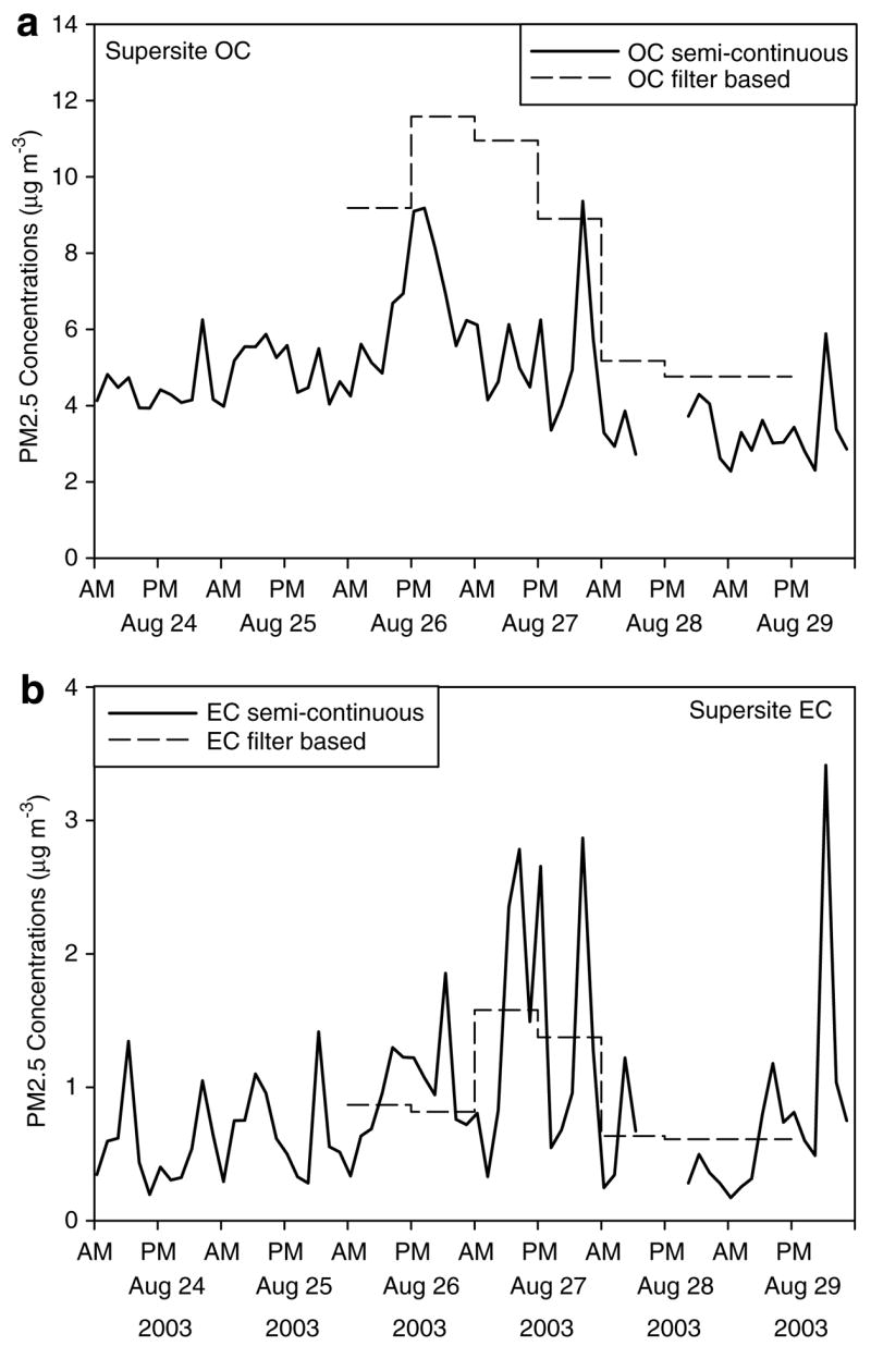
Comparison of OC (a) and EC (b) filter-based measurements with semi-continuous OCEC measurements at the urban background site (the St Louis Supersite).
Organic Speciation
The samples were analyzed individually by TD-GCMS. This method has been described in detail previously. Briefly, the filter is spiked with isotopically labeled internal standard and placed in a glass desorption tube. This tube fits into the autosampler for the Markes International Thermal Desorption Unit (model M-10140; Foster City, CA, USA) coupled with an Agilent Technologies5973 GCMS system. The internal standard and quantification standards used for this analysis comprise a range of PAHs, alkanes, hopanes and steranes designed to represent the range of compounds measured in ambient samples and to provide good surrogates for all of the compounds quantified in this method in the few cases when exact standards are not used. A three-point calibration curve is used for all compounds’ quantification, with a standard run every five samples to check the stability of the calibration curve. When this check standard does not pass the quality control check, the calibration curve is regenerated. The uncertainty is based on the percent relative standard deviation of check standard recoveries.
Source Apportionment
A CMB model (EPA-CMB version 8.2) was used to apportion OC from motor vehicle exhaust and cigarette smoke for each of the average job type, worksite area and urban background averages listed in Table 1a and b. Three different motor vehicle exhaust sources were used in the model; diesel exhaust, spark ignition exhaust and lubricating oil impacted exhaust, which are all taken from the same fleet study (Lough et al., 2007). The diesel profile is a weighted average of all weight class and driving cycle diesel exhaust based on the age of the fleet in the LA area (Lough and Schauer, 2007). The lubricating oil-impacted exhaust is taken from a “white smoker,” or normal-smoking gasoline vehicle, which has elevated lubricating oil markers (hopanes and steranes), but not elevated PAH or EC (Lough and Schauer, 2007). Smoking vehicles are often identified based on a visible smoke plume, which in the case of the “white smokers” are often a result of burning lubricating oil (Cadle et al., 1997; Sagebiel et al., 1997; Lough and Schauer, 2007), which is possible with both gasoline and diesel vehicles. Cigarette smoke apportionment has been performed using iso- and anteiso-alkanes as unique tracers (Schauer et al., 1996), but in this study, normal alkanes are considered indicators of cigarette smoke, using a previously published source profile (Hildemann et al., 1991; Rogge et al., 1994). The source profiles used in this study were analyzed by solvent extraction GCMS, whereas samples were analyzed using TD-GCMS. A previous study by Sheesley et al. has shown that these methods are compatible for the tracers used in the current study (Sheesley et al., 2007). The source emission profiles used in the CMB analysis used the same method for OCEC analysis (Schauer et al., 2003) as in the current study.
Table 1.
Concentrations of personal exposure and area sample averages by location.
| Dockworker
|
Mechanic
|
Hostler
|
Long-haul driver
|
P and D driver
|
|||||||||||
|---|---|---|---|---|---|---|---|---|---|---|---|---|---|---|---|
| n | 14 | 7 | 4 | 21 | 18 | ||||||||||
| μg m−3 | Ave | Unc | SD | Ave | Unc | SD | Ave | Unc | SD | Ave | Unc | SD | Ave | Unc | SD |
| (a) Personal exposure average concentrations by job title | |||||||||||||||
| OC | 13.00 | 1.02 | 2.92 | 19.78 | 1.45 | 5.81 | 13.35 | 1.12 | 7.48 | 24.05 | 1.66 | 8.75 | 17.98 | 1.30 | 6.80 |
| EC | 1.12 | 0.16 | 0.41 | 2.04 | 0.23 | 1.02 | 1.30 | 0.19 | 1.00 | 1.55 | 0.20 | 0.42 | 2.71 | 0.25 | 1.37 |
| ng m−3 | |||||||||||||||
| Benzo (b&k)fluoranthene | 0.04 | 0.01 | 0.03 | 0.30 | 0.05 | 0.19 | ND | 0.22 | 0.03 | 0.21 | 0.27 | 0.04 | 0.39 | ||
| Benzo(e) pyrene | 0.19 | 0.04 | 0.29 | 0.11 | 0.02 | 0.10 | ND | 0.11 | 0.02 | 0.09 | 0.30 | 0.06 | 0.30 | ||
| Benzo (a) pyrene | 0.04 | 0.01 | 0.01 | 0.19 | 0.05 | 0.07 | ND | 0.12 | 0.03 | 0.16 | 0.19 | 0.05 | 0.37 | ||
| Indeno (123-cd)pyrene | 0.08 | 0.02 | 0.10 | 0.05 | 0.01 | 0.02 | ND | 0.07 | 0.02 | 0.03 | 0.11 | 0.03 | 0.11 | ||
| Benzo (ghi) perylene | 1.15 | 0.37 | NA | ND | ND | ND | 0.81 | 0.26 | 0.38 | ||||||
| 22,29,30-trisnorneohopane | 0.20 | 0.03 | 0.13 | 0.32 | 0.05 | 0.46 | 0.22 | 0.03 | 0.17 | 0.48 | 0.07 | 0.39 | 0.31 | 0.04 | 0.15 |
| 17a(h)-21b(h)-29-Norhopane | 0.92 | 0.14 | 0.51 | 1.62 | 0.24 | 1.93 | 1.32 | 0.20 | 0.60 | 3.07 | 0.46 | 2.40 | 1.40 | 0.21 | 0.67 |
| 17a(H)-21b(h)-hopane | 0.50 | 0.06 | 0.29 | 0.87 | 0.10 | 0.93 | 0.72 | 0.09 | 0.19 | 1.40 | 0.17 | 1.10 | 0.68 | 0.08 | 0.32 |
| 22s-17a(H),21b(H)-30-Homohopane | 0.25 | 0.03 | 0.14 | 0.45 | 0.05 | 0.54 | 0.40 | 0.05 | 0.14 | 0.78 | 0.09 | 0.68 | 0.29 | 0.04 | 0.18 |
| 22R-17a(H),21b(H)-30-Homohopane | 0.18 | 0.02 | 0.11 | 0.34 | 0.04 | 0.37 | 0.31 | 0.04 | 0.10 | 0.57 | 0.07 | 0.48 | 0.21 | 0.03 | 0.13 |
| 20R, 5a(H), 14b(H), 17b(H)-cholestane | 0.30 | 0.04 | 0.24 | 0.42 | 0.06 | 0.48 | 0.33 | 0.04 | 0.17 | 0.95 | 0.12 | 0.64 | 0.41 | 0.05 | 0.19 |
| 20S, 5a(H), 14b(H), 17b(H)-cholestane | 0.14 | 0.02 | 0.11 | 0.18 | 0.03 | 0.16 | 0.17 | 0.03 | 0.08 | 0.40 | 0.06 | 0.27 | 0.21 | 0.03 | 0.09 |
| 20R, abb-sitostane | 0.18 | 0.02 | 0.16 | 0.31 | 0.04 | 0.36 | 0.25 | 0.03 | 0.07 | 0.55 | 0.07 | 0.43 | 0.22 | 0.03 | 0.14 |
| 20S, abb-sitostane | 0.22 | 0.03 | 0.18 | 0.34 | 0.05 | 0.37 | 0.27 | 0.04 | 0.06 | 0.59 | 0.08 | 0.45 | 0.22 | 0.03 | 0.14 |
| Tetracosane | 4.90 | 0.46 | 3.44 | 6.42 | 0.60 | 2.81 | 4.17 | 0.39 | 1.41 | 6.84 | 0.64 | 4.16 | 11.27 | 1.05 | 6.15 |
| Pentacosane | 4.23 | 0.56 | 3.21 | 4.99 | 0.67 | 1.90 | 4.05 | 0.54 | 0.44 | 5.69 | 0.76 | 4.55 | 7.17 | 0.96 | 3.14 |
| Hexacosane | 2.16 | 0.33 | 2.24 | 2.64 | 0.40 | 0.78 | 2.31 | 0.35 | 0.68 | 3.52 | 0.53 | 3.73 | 2.93 | 0.44 | 2.20 |
| Heptacosane | 3.11 | 0.59 | 1.99 | 10.47 | 1.98 | 14.22 | 5.20 | 0.99 | 4.58 | 14.60 | 2.77 | 22.34 | 4.37 | 0.83 | 6.75 |
| Octacosane | 1.24 | 0.23 | 0.98 | 2.67 | 0.51 | 2.80 | 1.93 | 0.36 | 1.05 | 3.27 | 0.62 | 4.13 | 1.47 | 0.28 | 1.48 |
| Nonacosane | 3.00 | 0.44 | 1.70 | 10.38 | 1.51 | 12.45 | 4.68 | 0.68 | 4.40 | 14.40 | 2.09 | 25.73 | 4.55 | 0.66 | 8.29 |
| Triacontane | 1.20 | 0.17 | 0.67 | 4.51 | 0.65 | 5.42 | 2.04 | 0.30 | 1.33 | 6.70 | 0.97 | 10.14 | 2.22 | 0.32 | 3.55 |
| Hentriacontane | 7.04 | 1.21 | 6.47 | 35.93 | 6.17 | 43.89 | 9.58 | 1.64 | 16.43 | 46.90 | 8.05 | 84.24 | 16.19 | 2.78 | 37.10 |
| Dotriacontane | 1.51 | 0.26 | 0.89 | 6.25 | 1.08 | 7.39 | 2.15 | 0.37 | 3.05 | 9.82 | 1.70 | 18.10 | 3.11 | 0.54 | 5.56 |
| Tritriacontane | 3.70 | 0.85 | 3.77 | 19.89 | 4.55 | 25.20 | 6.64 | 1.52 | 9.95 | 30.01 | 6.87 | 54.86 | 8.02 | 1.84 | 18.66 |
| Tetratriacontane | 0.21 | 0.06 | 0.21 | 1.19 | 0.34 | 1.21 | 0.85 | 0.24 | 0.26 | 3.54 | 1.00 | 2.92 | 0.93 | 0.26 | 0.78 |
| Pentriacontane | 0.03 | 0.01 | 0.02 | 0.17 | 0.06 | 0.14 | 0.09 | 0.04 | 0.05 | 0.24 | 0.09 | 0.17 | 0.07 | 0.02 | 0.05 |
| Dock | Shop | Yard | Urban background | ||||||||||||
| n | 14 | 8 | 6 | 9 | |||||||||||
| μg m−3 | Ave | Unc | SD | Ave | Unc | SD | Ave | Unc | SD | Ave | Unc | SD | |||
| (b) Area sample average concentrations by location | |||||||||||||||
| OC | 11.03 | 0.90 | 2.21 | 12.76 | 0.95 | 2.49 | 8.62 | 0.76 | 1.77 | 8.43 | 0.74 | 2.83 | |||
| EC | 1.18 | 0.15 | 0.38 | 1.97 | 0.18 | 0.82 | 1.19 | 0.15 | 0.38 | 0.94 | 0.14 | 0.34 | |||
| ng m−3 | |||||||||||||||
| Benzo (b&k)fluoranthene | 0.06 | 0.01 | 0.19 | 0.16 | 0.03 | 0.21 | ND | 0.07 | 0.01 | 0.05 | |||||
| Benzo(e)pyrene | 0.04 | 0.01 | 0.07 | 0.10 | 0.02 | 0.10 | 0.04 | 0.01 | 0.10 | 0.05 | 0.01 | 0.04 | |||
| Benzo(a)pyrene | 0.03 | 0.01 | 0.10 | 0.07 | 0.02 | 0.09 | ND | 0.003 | 0.001 | 0.01 | |||||
| Indeno(123-cd)pyrene | 0.08 | 0.02 | 0.21 | 0.10 | 0.02 | 0.10 | 0.00 | 0.00 | 0.01 | 0.03 | 0.01 | 0.05 | |||
| Benzo(ghi)perylene | 0.12 | 0.04 | 0.34 | 0.00 | 0.00 | 0.01 | 0.07 | 0.02 | 0.16 | 0.00 | 0.00 | 0.01 | |||
| 22,29,30-trisnorneohopane | 0.18 | 0.03 | 0.09 | 0.24 | 0.03 | 0.07 | 0.05 | 0.01 | 0.04 | 0.03 | 0.00 | 0.03 | |||
| 17a(h)-21b(h)-29-Norhopane | 0.84 | 0.13 | 0.27 | 0.92 | 0.14 | 0.21 | 0.57 | 0.09 | 0.31 | 0.30 | 0.04 | 0.14 | |||
| 17a(H)-21b(h)-hopane | 0.45 | 0.05 | 0.18 | 0.49 | 0.06 | 0.19 | 0.34 | 0.04 | 0.18 | 0.21 | 0.02 | 0.09 | |||
| 22s-17a(H),21b(H)-30-Homohopane | 0.23 | 0.03 | 0.11 | 0.24 | 0.03 | 0.13 | 0.19 | 0.02 | 0.12 | 0.09 | 0.01 | 0.06 | |||
| 22R-17a(H),21b(H)-30-Homohopane | 0.17 | 0.02 | 0.09 | 0.18 | 0.02 | 0.10 | 0.15 | 0.02 | 0.10 | 0.07 | 0.01 | 0.05 | |||
| 20R, 5a(H), 14b(H), 17b(H)-cholestane | 0.25 | 0.03 | 0.13 | 0.36 | 0.05 | 0.11 | 0.12 | 0.02 | 0.07 | 0.03 | 0.00 | 0.05 | |||
| 20S, 5a(H), 14b(H), 17b(H)-cholestane | 0.11 | 0.02 | 0.05 | 0.15 | 0.02 | 0.05 | 0.06 | 0.01 | 0.04 | 0.01 | 0.00 | 0.02 | |||
| 20R, abb-sitostane | 0.15 | 0.02 | 0.06 | 0.16 | 0.02 | 0.06 | 0.08 | 0.01 | 0.07 | 0.06 | 0.01 | 0.04 | |||
| 20S, abb-sitostane | 0.18 | 0.02 | 0.11 | 0.20 | 0.03 | 0.09 | 0.09 | 0.01 | 0.07 | 0.07 | 0.01 | 0.05 | |||
| Tetracosane | 5.31 | 0.49 | 3.08 | 7.86 | 0.73 | 2.82 | 1.44 | 0.13 | 1.05 | 1.54 | 0.14 | 1.31 | |||
| Pentacosane | 4.59 | 0.61 | 1.67 | 5.46 | 0.73 | 2.15 | 2.26 | 0.30 | 1.14 | 1.62 | 0.22 | 0.83 | |||
| Hexacosane | 2.29 | 0.35 | 1.67 | 2.09 | 0.32 | 0.85 | 0.98 | 0.15 | 0.63 | 0.48 | 0.07 | 0.50 | |||
| Heptacosane | 2.95 | 0.56 | 2.18 | 1.68 | 0.32 | 0.95 | 0.70 | 0.13 | 0.60 | 0.57 | 0.11 | 0.57 | |||
| Octacosane | 1.60 | 0.30 | 3.01 | 0.52 | 0.10 | 0.36 | 0.51 | 0.10 | 0.34 | 0.29 | 0.06 | 0.34 | |||
| Nonacosane | 2.80 | 0.41 | 2.84 | 1.36 | 0.20 | 0.92 | 0.54 | 0.08 | 0.21 | 0.47 | 0.07 | 0.49 | |||
| Triacontane | 1.28 | 0.19 | 1.92 | 0.65 | 0.09 | 0.89 | 0.08 | 0.01 | 0.07 | 0.22 | 0.03 | 0.27 | |||
| Hentriacontane | 6.05 | 1.04 | 6.79 | 3.26 | 0.56 | 2.42 | 0.64 | 0.11 | 0.63 | 0.45 | 0.08 | 0.52 | |||
| Dotriacontane | 0.97 | 0.17 | 0.90 | 0.66 | 0.11 | 0.82 | 0.05 | 0.01 | 0.07 | 0.17 | 0.03 | 0.22 | |||
| Tritriacontane | 3.31 | 0.76 | 3.81 | 1.72 | 0.39 | 1.64 | 0.53 | 0.12 | 0.45 | 0.21 | 0.05 | 0.27 | |||
| Tetratriacontane | 0.35 | 0.10 | 0.38 | 0.18 | 0.05 | 0.24 | 0.04 | 0.01 | 0.10 | 0.11 | 0.03 | 0.21 | |||
| Pentriacontane | 0.04 | 0.01 | 0.05 | 0.02 | 0.01 | 0.02 | 0.01 | 0.00 | 0.03 | 0.00 | 0.00 | 0.01 | |||
Ave, average of all job/area samples; EC, elemental carbon; NA, standard deviation not available because only one value; ND, not detected; OC, organic carbon; SD, standard deviation of all job/area samples; Unc, average analytical uncertainty for organic speciation.
Bold, these averages have a standard deviation that is less than half of the average (when considering the uncertainty).
Italics, these averages for the mechanics’ group have a standard deviation that is less than half of the average only when the sample individual EC 2203 is removed.
The OC apportionment results were then converted to EC apportionment results using EC-to-OC ratios from the emission source profiles used in the model. This enables assessment of the emission source contributions to EC concentrations at the freight terminal.
Results
Sample Averages
The samples were first evaluated by calculating averages for each sample type (Table 1a and b). This helps to determine the importance of worksite area or personal activity in the personal exposure samples, and whether each job type and each area type has a unique exposure profile. In Table 1, all of the averages for which the standard deviation of the average is equal to or less than 50% of the average are in bold (when including the analytical uncertainty). This is used as a rough split to separate groups that have less variability by sample, which would mean less impact by date, time or personal activity. In Figure 2a and b, the OC, EC and organic tracer concentrations for the personal exposure and worksite averages have been normalized by the urban background concentration (i.e., the personal exposure and worksite area concentrations have been divided by the urban background average). This effectively demonstrates the impact or enhancement due to the worksite area or job type, whereas a normalized concentration of 1 indicates that the personal exposure and the worksite area concentrations are on the same level as the urban background.
Figure 2.

Average concentration profiles of organic and elemental carbon (a) and organic tracers (b) normalized by urban background concentrations for each job type and worksite area. Error bars represent standard deviation of the average concentration for each species.
All of the job-type and area-type average OC concentrations have a standard deviation less than half of the average. Dockworkers and dock, shop and yard area samples have standard deviations nearly 20% of the average, which would indicate consistent OC concentrations within a group, but not necessarily identical OC source contributions. The average OC concentrations for the personal exposure samples are all higher than the worksite and urban background samples. The long-haul drivers’ OC concentrations, at 24 μgm−3, are almost twice as high as the highest area sample concentration (shop OC is 13 μgm−3 in Table 1). This indicates significant impact due to personal activity, which in this case includes exposure to roadway emissions and more personal sources such as cigarette smoke.
The average EC is similar to the OC in the consistency of EC among samples within a group (except for hostlers). However, unlike OC averages, EC personal exposure averages are only marginally elevated compared with the area samples, if elevated at all (1.18–1.97 μgm−3 for worksite areas and 1.12–2.71 μgm−3 for workers’ exposure in Table 1). Although long-haul drivers had by far the highest OC average, EC was closer in magnitude to that in the urban background. This is high lighted in Figure 2a and b, where the average concentrations have been normalized by the average urban background concentration for each sample type. The long-haul drivers, P and D drivers and mechanics have an average OC enhancement of 2–3 times higher than the urban background, but their EC enhancement does not follow the same pattern (Figure 2). While mechanics and P and D drivers have EC enhancements a factor of 2–3 of urban background, the long-haul drivers’ EC enrichment is only a factor of 1.5 over urban background.
The relative standard deviation is much higher for the molecular markers than for EC and OC. Only norhopane and hopane have standard deviations consistently at or below 50% for all worksite area samples and for dockworkers, hostlers and P and D drivers (Table 1). If one mechanic sample (EC2203) with hopane levels over four times higher than the next highest sample is removed, the mechanic hopane average has a relative standard deviation of 50% or less (with uncertainty). This indicates more consistency in the lubricating oil/motor vehicle source, for which hopanes are the markers, in most job and area types. The average personal exposure samples have significantly higher hopane levels than the area samples; the long-haul drivers had particularly high norhopane levels (average, 3.07 ngm−3), whereas the urban background are an order of magnitude lower at 0.30 ngm−3 (Table 1). This relationship will be explored by looking at correlations among the personal exposure and area samples. Long-haul drivers have high variability for all of the molecular markers, which might indicate that personal activity has a high impact for this job type. The wax n-alkanes, heptacosane to triacontane in particular, show very high variability for all the personal exposure samples; the heptacosane’s standard deviation is higher than the average for mechanics, long-haul drivers and P and D drivers (Table 1). The standard deviations of the organic tracers are particularly important when considering how representative average exposures are for each job type when conducting source apportionment. The long-haul driver average profile is less representative than the P and D driver average, when considering the relative standard deviations.
The differences among worker exposure and worksite areas are more pronounced for the organic tracers than OC or EC (Figure 2b). Normalized concentrations of PAHs are enriched by roughly an order of magnitude over the urban background for both dockworkers and P and D drivers, whereas mechanics and long-haul drivers are each a factor of four higher than urban background. Likewise, hopanes are enriched by an order of magnitude over urban background for long-haul drivers and 3–5 times higher than the urban background for the other workers. As mentioned previously, the tracers are uniformly greater than the urban background (except hostler PAH concentrations), with the wax alkanes, steranes and hopanes enriched in that order over the urban background in all personal exposures. Wax alkanes are enriched by an average of 50 times over the urban background for long-haul drivers(Figure 2b).
Urban Background and Worksite Correlations
The urban background, as represented by the Supersite samples, is plotted vs. the worksite area samples in Figure 3a–f to determine whether on-site sources or urban sources dominate freight terminal carbon concentrations. The urban background and worksite area samples are related in terms of bulk carbon concentrations (Figure 3a and b). The yard and dock measurements come closest to a 1:1 correlation, with the dock consistently biased high vs. the urban background. The shop area sample has the highest bias vs. the urban background for OC. The EC plots show more variability, particularly with shop samples; one sample’s concentration is almost three times higher than in it’s respective urban background sample. The worksite EC shows higher impact from worksite sources in addition to urban background than the worksite OC.
Figure 3.

Correlation plots of trucking terminal worksite area concentrations vs. the urban background for organic (a) and elemental (b) carbon, polycyclic aromatic hydrocarbons(c), hopanes(d), steranes(e) and alkanes(f).
The molecular-marker plots can be used to determine whether this relationship is determined by persistent emission sources (Figure 3c–f). There is no correlation among the worksite area samples and the urban background samples for PAHs, steranes and alkanes. For the PAHs, the concentrations are similar, but there is not a correlation. This would seem to indicate that although there is not a strong PAH emission source in the freight terminal, the PAHs at the Supersite are not directly transported to the trucking terminal. The steranes and alkanes are considerably higher in the worksite area samples, indicating strong freight terminal emission sources for both of these compound types. The hopanes have a completely different relationship than any of the other organic species, but are similar to EC. EC and hopanes potentially represent two different types of motor vehicle exhaust; EC represents diesel exhaust operating at high load (Kweon et al., 2002), whereas hopanes represent motor vehicle exhaust impacted by lubricating oil (Fraser et al., 2002; Kweon et al., 2002; Schauer et al., 2002), in this case idling or low load diesel. There is a strong correlation for the urban background vs. all the worksite area samples (0.72), but there is also a high slope (2.5) (Table 2). Thus, the urban background seems to have a consistent impact on the hopane concentration at the trucking terminal; however, this may simply be due to changes in intensity for PM concentrations at all locations primarily due to meteorology.
Table 2.
Regression statistics for work site area vs. job type samples.
| EC | Hopanes | Ave ratio (personal:area) EC | Ave ratio (personal:area) Hopanes | |
|---|---|---|---|---|
| Supersite vs. freight terminal | ||||
| Intercept | NA | −0.02 | ||
| Slope | NA | 2.53 | ||
| r2 | NA | 0.72 | ||
| Dock vs. dockworkera | ||||
| Intercept | 0.38 | 0.03 | 0.94 | 1.11 |
| Slope | 0.63 | 1.09 | ||
| r2 | 0.12 | 0.57 | ||
| Shop vs. mechanicb | ||||
| Intercept | −0.42 | 0.30 | 1.04 | 1.77 |
| Slope | 1.38 | 0.88 | ||
| r2 | 0.85 | 0.08 | ||
| Yard vs. hostlers | ||||
| Intercept | NA | 0.18 | 1.09 | 2.23 |
| Slope | NA | 1.50 | ||
| r2 | NA | 0.42 | ||
| Yard vs. P and D | ||||
| Intercept | −0.74 | 0.01 | 2.27 | 2.11 |
| Slope | 3.16 | 2.61 | ||
| r2 | 0.20 | 0.55 | ||
| Urban background vs. P and D | ||||
| Intercept | 0.27 | 0.04 | 2.87 | 4.08 |
| Slope | 2.73 | 3.94 | ||
| r2 | 0.29 | 0.57 | ||
| Urban background vs. long haul | ||||
| Intercept | NA | 0.20 | 1.65 | 9.06 |
| Slope | NA | 8.27 | ||
| r2 | NA | 0.26 | ||
EC, elemental carbon; NA, no regression calculated/no relationship apparent.
Bold, r2>0.60.
If dockworker D8 was removed for regression statistics, the r2 would be 0.63 for hopanes, with a slope of 1.15.
If mechanicM2 was removed for regression statistics, the r2 would be 0.80 for hopanes, with a slope of 0.86.
Personal Exposure and Area Sample Correlations
Personal exposure samples are plotted against their respective worksite area sample in Figures 4 and 5 and in Supplementary Figures S1 and S2. The drivers’ exposure concentrations (hostlers, P and D, and long haul) are plotted against the urban background. These plots indicate the relationship between worksite area concentrations and personal exposures. As outlined in the model, occupational personal exposure is a sum of urban background, worksite and personal activities. For the on-site workers at the freight terminal, this is a clear model, as three components (personal exposure, worksite area concentrations and urban background) can be measured. However, for the off-site drivers, only urban background and personal exposure have been measured. Sampling the off-site drivers’ worksite contribution would be impractical, as their worksite area is the roadway; roadway contribution is not constant and could not easily be represented by a sampler at a static site (Phuleria et al., 2007). Therefore, driver exposure is considered the sum of urban background and the combined roadway/personal activity. In light of this, the driver exposure concentrations are plotted against the urban background to assess the background contribution.
Figure 4.

Correlation plots of dockworker exposures vs. dock area concentrations for organic (a) and elemental (b) carbon, polycyclic aromatic hydrocarbons (c), hopanes (d) and alkanes where smoking status is listed (e). Error bars represent analytical uncertainty.
Figure 5.

Correlation plots of driver exposures vs. the urban background for organic (a) and elemental (b) carbon, polycyclic aromatic hydrocarbons (c), hopanes (d) and alkanes where smoking status is listed (e). Error bars represent analytical uncertainty.
In addition to OC, molecular marker concentrations(EC, hopanes, alkanes and PAHs) are plotted to indicate which sources are more impacted by personal activity or cannot be easily represented by a surrogate ambient or worksite area measurement, which would potentially include roadway exposure. The regression statistics in Figures 4 and 5 and Supplementary Figures S1 and S2 are included in Table 2. Only those plots, which demonstrated a visual relationship were included in the table.
On-site Jobs: Dockworkers, Mechanics and Hostlers
For the dock vs. dockworker plots, OC does not show a clear correlation, although overall concentrations are very similar (Table 1a and b; Figure 4a). Hopanes and EC both have ratios of nearly 1 for the worksite area:personal exposure relationship (Table 2). One personal exposure sample appeared to be an outlier, EC concentration was near zero and hopane levels were also very low, which had an impact on the hopane regression statistics; the correlation coefficient for hopanes improved to 0.63 when this one point was removed. Overall, the dock concentration of diesel indicators (EC and hopanes) represents the personal exposure of dockworkers moderately well.
The alkanes show considerable variation among sample pairs, and in some cases have levels much higher than the dock area sample. In the samples where the alkane levels were systematically high, iso- and anteiso-alkanes levels were also high. These branched alkanes are not specifically quantified by TD-GCMS, but will be added in the future as they can function as important markers for cigarette smoke (Rogge et al., 1994; Kavouras et al., 1998). It follows then, in the personal exposure samples in this study, that high alkanes can be considered indicative of cigarette smoke. PAHs are very low in both the dock area and dockworker samples, and are similar to the urban background measurements, as mentioned previously.
For mechanics, the shop area sample is a good representation of the mechanics’ exposure to motor vehicle exhaust as represented by both EC and hopanes (for all but the one individual). Organic carbon, PAHs and alkanes show similar lack of correlation between personal and area samples as was seen for the dockworkers. There are not many mechanic samples; however, the relationships are very clear for both EC and hopanes(Supplementary Figure S1; Supplementary Materials); both species have average ratios near 1 (Table 2). For hopanes, if the one mechanic sample with high concentration was removed from the regression calculation for hopanes, the correlation coefficient becomes 0.80, with a slope of 0.86; this individual’s EC concentration was in line with the remainder of the mechanics’ (Supplementary Figure S1) and did not distort the EC regression statistics. This individual’s personal activity generated a much higher concentration of the same lube oil/motor vehicle source represented by the remaining mechanic and shop area samples. Because this study is more interested in defining the average or most typical relationships, the statistics which omit that individual will be used in all further discussions.
With only four hostler samples, good statistical information cannot be expected; however, hopanes and EC do show patterns similar to the mechanics for the yard area:hostler relationship (Supplementary Figures S1 and S2). The correlation coefficient for the hopanes is nearly 0.4 for the yard (Table 2).
Off-site Jobs: P and D and Long-Haul Drivers
The two sets of drivers operate in similar on-road conditions but on different spatial scales: P and D drivers operate on the local scale within cities and suburban areas and the long-haul drivers operate on more of a regional scale between cities. They have been combined for the correlation analysis in Figure 5a–f, with black squares representing long haul and white squares representing P and D drivers, but are separate in the correlation statistics (Table 2).
For P and D drivers, the loadings are consistently much higher for personal exposure samples as compared with the urban background for all measured species (Table 2). Although there is a slight correlation between the urban background area samples and the P and D driver samples for EC, the relationship is stronger for hopanes. The alkanes are impacted by personal activity as with all the personal exposure samples. The PAHs are consistently higher for the P and D driver compared with either the yard or urban background, which indicates a source specific to these drivers, such as in-traffic exposures.
The long-haul drivers show the least correlation to any area samples of any job type (Figure 5). There is only a small correlation for hopanes and the slopes are quite high (m=8.3 for the urban background). As with P and D drivers, the concentrations for all species are significantly higher than the urban background concentrations. Unlike the rest of the drivers and terminal workers, there is a large difference between the average worksite area: worker exposure ratios for EC and hopanes(T able 2); the EC ratio is only 1.65 compared with over 9 for hopanes. The long-haul drivers are not experiencing the same sources as the St Louis urban background or trucking terminal; this is not unexpected as they spend a significant portion of their time driving outside the city.
The yard and urban background hopanes are a fraction of the lube oil/motor vehicle exhaust source for the drivers, but the roadway microenvironment increases this source. Because the drivers are exposed to motor vehicle traffic outside of the trucking terminal, it cannot be determined from this data whether the lube oil/motor vehicle source for the drivers is diesel smokers (high OC emitters), gasoline exhaust (including gasoline smokers) or a mixture.
Source Apportionment
The CMB modeling was focused on motor vehicle and cigarette smoke contributions to organic carbon PM, as only the non-polar tracers were measured. Levoglucosan is necessary to accurately apportion wood smoke and it requires polar GCMS methods. The results of this limited CMB are presented in Figure 6a and Table 3, where unapportioned OC mass would include wood smoke, secondary organic carbon and resuspended dust. Cigarette smoke was apportioned using normal or n-alkanes for the job type, dock and shop average profiles; n-alkanes levels were 7–40 times higher than in the yard samples for personal exposure averages. Since n-alkanes can be emitted from a variety of sources in the ambient environment, this source was not calculated for yard or urban background averages. The source apportionment modeling used the job type and worksite area averages shown in Table 1a and b. These results are therefore impacted by the variability within each sample type as depicted by the reported standard deviations.
Figure 6.

CMB results for carbon contributions of mobile sources and cigarette smoke for each job type, worksite and the urban background; (a) OC source apportionment, (b) EC source apportionment. Error bars represent uncertainty of OC measurement.
Table 3.
Results with model uncertainty for OC (μgm−3 OC) and EC apportionment (μgm−3 EC).
| OC apportionment | Cigarette smoke | Unc | Diesel | Unc | Spark ignition | Unc | Lubricating oil-impacted exhaust | Unc | Unapportioned | Total OC | Unc |
|---|---|---|---|---|---|---|---|---|---|---|---|
| Dockworker | 0.60 | 0.06 | 0.37 | 0.07 | 0.45 | 0.13 | 3.67 | 0.32 | 7.91 | 13.00 | 1.02 |
| Mechanic | 2.06 | 0.21 | 0.71 | 0.11 | 0.30 | 0.09 | 5.88 | 0.48 | 10.85 | 19.78 | 1.45 |
| Hostler | 0.90 | 0.10 | 0.37 | 0.11 | 0.97 | 0.81 | 4.33 | 0.89 | 6.72 | 13.35 | 1.12 |
| Long-haul driver | 2.77 | 0.30 | 0.47 | 0.09 | 0.38 | 0.12 | 10.19 | 0.82 | 10.19 | 24.05 | 1.66 |
| P and D driver | 1.06 | 0.11 | 0.98 | 0.13 | 0.60 | 0.17 | 4.61 | 0.42 | 10.75 | 17.98 | 1.30 |
| Dock | 0.53 | 0.06 | 0.43 | 0.07 | 0.16 | 0.06 | 3.45 | 0.29 | 6.42 | 11.03 | 0.90 |
| Shop | 0.27 | 0.03 | 0.73 | 0.10 | 0.44 | 0.15 | 3.74 | 0.34 | 7.63 | 12.76 | 0.95 |
| Yard | 0.00 | 0.00 | 0.45 | 0.07 | 0.00 | 0.04 | 2.36 | 0.22 | 5.79 | 8.62 | 0.76 |
| Urban background | 0.00 | 0.00 | 0.34 | 0.06 | 0.22 | 0.06 | 0.76 | 0.10 | 7.08 | 8.43 | 0.74 |
| EC apportionment | Cigarette smoke | Unc | Diesel | Unc | Spark ignition | Unc | Lubricating oil-impacted exhaust | Unc | Unapportioned | EC | ECU |
|
| |||||||||||
| Dockworker | 0.00 | 0.00 | 0.95 | 0.18 | 0.13 | 0.04 | 0.07 | 0.01 | −0.04 | 1.12 | 0.16 |
| Mechanic | 0.02 | 0.00 | 1.82 | 0.28 | 0.09 | 0.03 | 0.11 | 0.01 | 0.01 | 2.04 | 0.23 |
| Hostler | 0.01 | 0.00 | 0.95 | 0.29 | 0.28 | 0.23 | 0.08 | 0.02 | −0.02 | 1.30 | 0.19 |
| Long haul | 0.02 | 0.00 | 1.21 | 0.24 | 0.11 | 0.03 | 0.20 | 0.02 | 0.02 | 1.55 | 0.20 |
| P and D | 0.01 | 0.00 | 2.51 | 0.34 | 0.17 | 0.05 | 0.09 | 0.01 | −0.08 | 2.71 | 0.25 |
| Dock | 0.00 | 0.00 | 1.11 | 0.18 | 0.05 | 0.02 | 0.07 | 0.01 | −0.04 | 1.18 | 0.15 |
| Shop | 0.00 | 0.00 | 1.86 | 0.25 | 0.13 | 0.04 | 0.07 | 0.01 | −0.09 | 1.97 | 0.18 |
| Yard | 0.00 | 0.00 | 1.15 | 0.18 | 0.00 | 0.01 | 0.05 | 0.01 | 0.00 | 1.19 | 0.15 |
| Urban background | 0.00 | 0.00 | 0.86 | 0.16 | 0.06 | 0.02 | 0.02 | 0.01 | 0.00 | 0.94 | 0.14 |
OC, organic carbon; EC, elemental carbon; P and D, pickup and delivery; Unc, uncertainty calculated in the model based on model fit.
Three different profiles were used for the mobile source emissions (Lough et al., 2007), as detailed under Methods. Most of the motor vehicle contribution was attributed to the lubricating oil-impacted exhaust; this follows the trends seen in Figure 2a and b where the EC is at most enriched three times over the urban background, whereas hopanes are enriched up to 10 times over the urban background. The worksite area exposure for mobile sources can be calculated by subtracting the urban background from each of the worker exposure and worksite area average contributions. Lubricating oil-impacted exhaust contributions range from roughly 3 to 9 μgm−3 of OC for worker exposure after subtracting urban background; dockworkers, hostlers and P and D driver averages have personal exposures at around 3 μgm−3 of OC, whereas the mechanic average is5 μgm−3 and the long-haul average exposure is roughly 9 μgm−3 of OC. The lubricating oil-impacted exhaust is by far the largest worksite area contribution for on-site and off-site workers.
An EC apportionment was then calculated using the OC model results and the EC to OC ratio from the emission source profiles (Figure 6b). The calculated to measured ratios for EC within the OC CMB model were within 0.9–1.25. The EC apportionment results look quite different than the OC apportionment results with most of the EC apportioned to diesel exhaust with a smaller percentage from spark ignition and lubricating oil-impacted EC. The EC apportionment illustrates that it is reasonable to assume that almost all of the EC in the trucking terminal-based jobs and in driver exposure is from diesel sources. However, the OC apportionment, which shows large contributions from lubricating oil-impacted exhaust, illustrates that occupational diesel exposure contains a significant OC component that may not be tracked effectively by only measuring EC concentrations.
Discussion
This data set provides an excellent base for the discussion of important questions, for example how well does an occupational area sample (local urban or indoor) represent personal exposure and does this vary by source? This question is particularly relevant in reference to the proposed personal exposure model: Personal exposure=urban background+ worksite background + personal activity. Do EC and hopanes track the same motor vehicle source within a diesel-impacted environment? How representative are the personal exposure averages by job type?
For the first question, this data set provides a unique continuum. At one end the mechanics are in the most contained environment where the two markers for motor vehicle exhaust, hopanes and EC, show clear correlations and a near one-to-one relationship in the worksite area and personal exposure samples. At the opposite end are the long-haul drivers who operate on a regional scale and have only a small correlation for the most specific motor vehicle marker, hopanes. In the paradigm of the personal exposure model, personal activity dominates when that activity is close to emission sources, whereas worksite contributions dominate when the sources are dispersed within a well characterized work environment. As evidenced in all of the personal exposure samples, cigarette smoke (as represented quantitatively by alkanes and qualitatively by iso- and ante-isoalkanes) is dominated exclusively by personal activity. In this context, personal activity includes both personal smoking and proximity to smokers, as evidenced in Figures 4e and 5e. In these two figures only, the smoking status of the workers has been included, when available. For the drivers, exposure to cigarette smoke is linked directly to personal smoking status, since the sampler was located in the truck cab. For the dockworkers, each participant wore a personal sampler and elevated alkane concentrations were observed in both smokers and in some non-smokers compared with dock background samples. This pattern suggests a source of exposure to cigarette smoke not attributable to personal smoking in some dockworkers. Dockworkers have the least difference between personal exposure and the dock measurement for alkanes, but there is still no correlation. As mentioned previously, the measurement of organic tracers is integral for defining the worksite vs. personal exposure relationship as OC concentrations are not a sufficiently specific measurement and OC emission sources are not uniformly impacted by personal activity.
An overall assessment of all the personal exposure, worksite area and urban background samples indicates that hopanes and EC do not necessarily depict the same source. The slopes and average ratios for hopanes and EC are most similar for the on-site workers, including dockworkers and mechanics, which indicates some uniformity in the on-site diesel profile. However, long-haul drivers illustrate the opposite extreme, with the EC at nearly ambient concentrations, whereas the hopanes enriched by a factor of 9 vs. the urban background. Thus, EC measurement would not be sufficient to depict the lube oil/motor vehicle exhaust component of the diesel source among all freight terminal workers. This is further illustrated in the OC and EC source apportionment results; these are significantly different in that the dominant OC source is lubricating oil-impacted exhaust, whereas the dominant EC source is diesel exhaust. Lubricating oil-impacted exhaust could include both diesel and gasoline exhaust, particularly in the off-site driver exposures.
The final question on whether the average profiles are representative is important for extrapolating beyond this study to diesel exposure within truck terminals and truck driver exposure. For most of the workers, the standard deviation for the major motor vehicle tracers (EC and hopanes) was less than 50% of the average, whereas that for long-haul driver hopanes was well over 50% of the average. Thus inter -city driving exposure is much harder to predict than intra-city driving exposure, but only for the hopane-monitored lube oil component of motor vehicle exhaust. A larger sample set may help to further define the average long-haul truck driver exposure to the lube oil/organic carbon component of motor vehicle exhaust. The source apportionment component of the study provides an estimate of the average mobile source exposure for each job type and worksite area. The mobile source OC could be smoking gasoline motor vehicles or diesel engines operating at low-load conditions (Kweon et al., 2003; Lough et al., 2007), but it contributed 3–9 μgm−3 of OC over the urban background for all of the job types. These results confirm the dominance of the hopane-tracked, lubricating oil-impacted exhaust source for the total trucking terminal worksite area and the drivers OC exposures when compared with the urban background. The EC apportionment confirms that almost all of the EC measured in the trucking industry is due to diesel exhaust. The OC apportionment reveals that OC has a considerably higher diesel/mobile source mass contribution than EC, which may need to be considered in exposure and health studies, as it may not be effectively traced by simply measuring EC concentration.
Supplementary Material
Supplementary Information accompanies the paper on the Journal of Exposure Analysis and Environmental Epidemiology website (http://www.nature.com/jes)
Acknowledgments
This sampling and organic and elemental analysis were funded by NIH/NCI R01 CA90792 and the organic speciation analysis was funded by HEI 4705-RFA03–1/04-1. We acknowledge the work by Mark Meirtiz at the Wisconsin State Laboratory of Hygiene in assisting in the development of the TD-GCMS method used in this study. We thank Jay Turner for assistance in coordinating sample collection at the St Louis Supersite. We also thank the International Brotherhood of Teamsters Safety and Health Dept. (LaMont Byrd) and the participating companies.
References
- Bae MS, Schauer JJ, DeMinter JT, Turner JR. Hourly and daily patterns of particle-phase organic and elemental carbon concentrations in the urban atmosphere. J Air Waste Manage Assoc. 2004a;54(7):823–833. doi: 10.1080/10473289.2004.10470957. [DOI] [PubMed] [Google Scholar]
- Bae MS, Schauer JJ, DeMinter JT, Turner JR, Smith D, Cary RA. Validation of a semi-continuous instrument for elemental carbon and organic carbon using a thermal-optical method. Atmos Environ. 2004b;38(18):2885–2893. [Google Scholar]
- Bae MS, Schauer JJ, Turner JR. Estimation of the monthly average ratios of organic mass to organic carbon for fine particulate matter at an urban site. Aerosol Sci Technol. 2006;40(12):1123–1139. [Google Scholar]
- Bailey CR, Somers JH, Steenland K. Exposures to diesel exhaust in the International Brotherhood of Teamsters, 1950–1990. AIHA J. 2003;64(4):472–479. doi: 10.1202/435.1. [DOI] [PubMed] [Google Scholar]
- Baulig A, Garlatti M, Bonvallot V, Marchand A, Barouki R, Marano F, et al. Involvement of reactive oxygen species in the metabolic pathways triggered by diesel exhaust particles in human airway epithelial cells. Am J Physiol Lung Cell Mol Physiol. 2003;285(3):L671–L679. doi: 10.1152/ajplung.00419.2002. [DOI] [PubMed] [Google Scholar]
- Cadle SH, Mulawa PA, Ball J, Donase C, Weibel A, Sagebiel JC, et al. Environ Sci Technol. 1997;31(12):3405–3412. [Google Scholar]
- Cohen HJ, Borak J, Hall T, Sirianni G, Chemerynski S. Exposure of minersto diesel exhaust particulates in underground nonmetal mines. AIHA J. 2002;63(5):651–658. doi: 10.1080/15428110208984753. [DOI] [PubMed] [Google Scholar]
- Davis ME, Smith TJ, Laden F, Hart JE, Ryan LM, Garshick E. Modeling particle exposure in US trucking terminals. Environ Sci Technol. 2006;40(13):4226–4232. doi: 10.1021/es052477m. [DOI] [PMC free article] [PubMed] [Google Scholar]
- Delfino RJ, Sioutas C, Malik S. Potential role of ultrafine particles in associations between airborne particle mass and cardiovascular health. Environ Health Perspect. 2005;113(8):934–946. doi: 10.1289/ehp.7938. [DOI] [PMC free article] [PubMed] [Google Scholar]
- Fraser MP, Lakshmanan K, Fritz SG, Ubanwa B. Variation in composition of fine particulate emissions from heavy-duty diesel vehicles. J Geophys Res Atmos. 2002;107(D21):8346. [Google Scholar]
- Garshick E, Laden F, Hart JE, Rosner B, Smith TJ, Dockery DW, et al. Lung cancer in railroad workers exposed to diesel exhaust. Environ Health Perspect. 2004;112(15):1539–1543. doi: 10.1289/ehp.7195. [DOI] [PMC free article] [PubMed] [Google Scholar]
- Garshick E, Laden F, Hart JE, Smith TJ, Rosner B. Smoking imputation and lung cancer in railroad workers exposed to diesel exhaust. Am J Ind Med. 2006;49(9):709–718. doi: 10.1002/ajim.20344. [DOI] [PMC free article] [PubMed] [Google Scholar]
- Garshick E, Schenker MB, Munoz A, Segal M, Smith TJ, Woskie SR, et al. A case–control study of lung-cancer and diesel exhaust exposure in railroad workers. Am Rev Respir Dis. 1987;135(6):1242–1248. doi: 10.1164/arrd.1987.135.6.1242. [DOI] [PubMed] [Google Scholar]
- Garshick E, Schenker MB, Munoz A, Segal M, Smith TJ, Woskie SR, et al. A retrospective cohort study of lung-cancer and diesel exhaust exposure in railroad workers. Am Rev Respir Dis. 1988;137(4):820–825. doi: 10.1164/ajrccm/137.4.820. [DOI] [PubMed] [Google Scholar]
- Geller MD, Ntziachristos L, Mamakos A, Samaras Z, Schmitz DA, Froines JR, et al. Physicochemical and redox characteristics of particulate matter (PM) emitted from gasoline and diesel passenger cars. Atmos Environ. 2006;40(36):6988–7004. [Google Scholar]
- Hart JE, Laden F, Schenker MB, Garshick E. Chronic obstructive pulmonary disease mortality in diesel-exposed railroad workers. Environ Health Perspect. 2006;114(7):1013–1017. doi: 10.1289/ehp.8743. [DOI] [PMC free article] [PubMed] [Google Scholar]
- Hildemann LM, Markowski GR, Cass GR. Chemical-composition of emissions from urban sources of fine organic aerosol. Environ Sci Technol. 1991;25(4):744–759. [Google Scholar]
- Hirano S, Furuyama A, Koike E, Kobayashi T. Oxidative-stress potency of organic extracts of diesel exhaust and urban fine particles in rat heart microvessel endothelial cells. Toxicology. 2003;187(2–3):161–170. doi: 10.1016/s0300-483x(03)00053-2. [DOI] [PubMed] [Google Scholar]
- Hoffmann B, Jockel KH. Diesel exhaust and coal mine dust – lung cancer risk in occupational settings. In: Mehlman M, Soffritti M, Landrigan P, Bingham E, Belpoggi F, editors. Living in a Chemical World: Framing the Future in Light of the Past. Wiley-Blackwell; Boston, Massachusetts: 2006. pp. 253–265. [Google Scholar]
- Jaeckels JM, Bae MS, Schauer JJ. Positive matrix factorization (PMF) analysis of molecular marker measurements to quantify the sources of organic aerosols. Environ Sci Technol. 2007;41(16):5763–5769. doi: 10.1021/es062536b. [DOI] [PubMed] [Google Scholar]
- Kavouras IG, Stratigakis N, Stephanou EG. Iso- and anteiso-alkanes: specific tracers of environmental tobacco smoke in indoor and outdoor particle size distributed urban aerosols. Environ Sci Technol. 1998;32(10):1369–1377. [Google Scholar]
- Kweon C, Okada S, Foster DE, Bae M, Schauer JJ. Effect of engine operating conditions on particle-phase organic compounds in engine exhaust of a heavy-duty direct-injection (DI) diesel engine 2003-01-0342 SAE Technical Paper Series, Society of Automotive Engineers. 2003 [Google Scholar]
- Kweon C, Okada S, Schauer JJ, Foster DE. Detailed chemical composition and particle size assessment of diesel engine exhaust 2002-01-2670: SAE Technical Paper Series, Society of Automotive Engineers. 2002 [Google Scholar]
- Lough GC, Christenson CC, Schauer JJ, Tortorelli JJ, Bean E, Lawson DR, et al. Development of molecular marker source profiles for emissions from on-road gasoline and diesel vehicle fleets. J Air Waste Manag Assoc. 2007;57(10):1190–1199. doi: 10.3155/1047-3289.57.10.1190. [DOI] [PubMed] [Google Scholar]
- Lough GC, Schauer JJ. Sensitivity of source apportionment of urban particulate matter to uncertainty in motor vehicle emission profiles. J Air Waste Manag Assoc. 2007;57(10):1200–1213. doi: 10.3155/1047-3289.57.10.1200. [DOI] [PubMed] [Google Scholar]
- Mader BT, Schauer JJ, Seinfeld JH, Flagan RC, Yu JZ, Yang H, et al. Sampling methods used for the collection of particle-phase organic and elemental carbon during ACE-Asia. Atmos Environ. 2003;37(11):1435–1449. [Google Scholar]
- McDonald JD, Eide I, Seagrave J, Zielinska B, Whitney K, Lawson DR, et al. Relationship between composition and toxicity of motor vehicle emission samples. Environ Health Perspect. 2004;112(15):1527–1538. doi: 10.1289/ehp.6976. [DOI] [PMC free article] [PubMed] [Google Scholar]
- Phuleria HC, Sheesely RJ, Schauer JJ, Fine PM, Sioutas C. Roadside measurements of size-segregated particulate organic compounds near gasoline and diesel-dominated freeways in Los Angeles, CA. Atmos Environ. 2007;41(22):4653–4671. [Google Scholar]
- Reed MD, Gigliotti AP, McDonald JD, Seagrave JC, Seilkop SK, Mauderly JL. Health effects of subchronic exposure to environmental levels of diesel exhaust. Inhal Toxicol. 2004;16(4):177–193. doi: 10.1080/08958370490277146. [DOI] [PubMed] [Google Scholar]
- Rogge WF, Hildemann LM, Mazurek MA, Cass GR. Sources of fine organic aerosol. 6. Cigarette smoke in the urban atmosphere. Environ Sci Technol. 1994;28(7):1375–1388. doi: 10.1021/es00056a030. [DOI] [PubMed] [Google Scholar]
- Sagebiel JC, Zielinska B, Walsh PA, Chow JC, Cadle SH, Mulawa PA, et al. PM-10 exhaust samples collected during IM-240 dynamometer tests of in-service vehicles in Nevada. Environ Sci Technol. 1997;31(1):75–83. [Google Scholar]
- Sarnat JA, Koutrakis P, Suh HH. Assessing the relationship between personal particulate and gaseous exposures of senior citizens living in Baltimore MD. J Air Waste Manag Assoc. 2000;50(7):1184–1198. doi: 10.1080/10473289.2000.10464165. [DOI] [PubMed] [Google Scholar]
- Sarnat SE, Coull BA, Schwartz J, Gold DR, Suh HH. Factors affecting the association between ambient concentrations and personal exposures to particles and gases. Environ Health Perspect. 2006;114(5):649–654. doi: 10.1289/ehp.8422. [DOI] [PMC free article] [PubMed] [Google Scholar]
- Schauer JJ. Evaluation of elemental carbon as a marker for diesel particulate matter. J Expo Anal Environ Epidemiol. 2003;13(6):443–453. doi: 10.1038/sj.jea.7500298. [DOI] [PubMed] [Google Scholar]
- Schauer JJ, Kleeman MJ, Cass GR, Simoneit BRT. Measurement of emissions from air pollution sources. 2. C1 through C30 organic compounds from medium duty diesel trucks. Environ Sci Technol. 1999;33(10):1578–1587. [Google Scholar]
- Schauer JJ, Kleeman MJ, Cass GR, Simoneit BRT. Measurement of emissions from air pollution sources. 5. C-1–C-32 organic compounds from gasoline-powered motor vehicles. Environ Sci Technol. 2002;36(6):1169–1180. doi: 10.1021/es0108077. [DOI] [PubMed] [Google Scholar]
- Schauer JJ, Mader BT, Deminter JT, Heidemann G, Bae MS, Seinfeld JH, et al. ACE-Asia intercomparison of a thermal-optical method for the determination of particle-phase organic and elemental carbon. Environ Sci Technol. 2003;37(5):993–1001. doi: 10.1021/es020622f. [DOI] [PubMed] [Google Scholar]
- Schauer JJ, Rogge WF, Hildemann LM, Mazurek MA, Cass GR, Simoneit BRT. Source apportionment of airborne particulate matter using organic compounds as tracers. Atmos Environ. 1996;30(22):3837–3855. [Google Scholar]
- Seagrave J, Mauderly JL, Seilkop SK. In vitro relative toxicity screening of combined particulate and semivolatile organic fractions of gasoline and diesel engine emissions. J Toxicol Environ Health. 2003;66(12):1113–1132. doi: 10.1080/15287390390213881. [DOI] [PubMed] [Google Scholar]
- Seagrave J, McDonald JD, Bedrick E, Edgerton ES, Gigliotti AP, Jansen JJ, et al. Lung toxicity of ambient particulate matter from southeastern US sites with different contributing sources: Relationships between composition and effects. Environ Health Perspect. 2006;114(9):1387–1393. doi: 10.1289/ehp.9234. [DOI] [PMC free article] [PubMed] [Google Scholar]
- Sheesley RJ, Schauer JJ, Meiritz MM, Deminter JT, Bae MS, Turner JR. Daily variation in particle-phase source tracers in an urban atmosphere. Aerosol Sci Technol. 2007;41(11):981–993. [Google Scholar]
- Sioutas C, Delfino RJ, Singh M. Exposure assessment for atmospheric ultrafine particles (UFPs) and implications in epidemiologic research. Environ Health Perspect. 2005;113(8):947–955. doi: 10.1289/ehp.7939. [DOI] [PMC free article] [PubMed] [Google Scholar]
- Smith TJ, Davis ME, Reaser P, Natkin J, Hart JE, Laden F, et al. Overview of particulate exposures in the US trucking industry. J Environ Monit. 2006;8(7):711–720. doi: 10.1039/b601809b. [DOI] [PMC free article] [PubMed] [Google Scholar]
- Stayner L, Bailer AJ, Smith R, Gilbert S, Rice F, Kuempel E. Uncertainty in the Risk Assessment of Environmental and Occupational Hazards. Vol. 895. New York Academy of Sciences; New York: 1999. Sources of uncertainty in dose-response modeling of epidemiological data for cancer risk assessment; pp. 212–222. [DOI] [PubMed] [Google Scholar]
- Violante FS, Barbieri A, Curti S, Sanguinetti G, Graziosi F, Mattioli S. Urban atmospheric pollution; personal exposure versus fixed monitoring station measurements. Chemosphere. 2006;64:1722–1729. doi: 10.1016/j.chemosphere.2006.01.011. [DOI] [PubMed] [Google Scholar]
- Woskie SR, Smith TJ, Hammond SK, Schenker MB, Garshick E, Speizer FE. Estimation of the diesel exhaust exposures of railroad workers. 1. Current exposures. Am J Ind Med. 1988;13(3):381–394. doi: 10.1002/ajim.4700130307. [DOI] [PubMed] [Google Scholar]
- Zaebst DD, Clapp DE, Blade LM, Marlow DA, Steenland K, Hornung RW, et al. Quantitative-determination of trucking industry workers exposures to diesel exhaust particles. Am Ind Hyg Assoc J. 1991;52(12):529–541. doi: 10.1080/15298669191365162. [DOI] [PubMed] [Google Scholar]
Associated Data
This section collects any data citations, data availability statements, or supplementary materials included in this article.
Supplementary Materials
Supplementary Information accompanies the paper on the Journal of Exposure Analysis and Environmental Epidemiology website (http://www.nature.com/jes)