

Abstract
During functional MRI (fMRI) studies, blood oxygenation-level dependent (BOLD) signal associated with neuronal activity acquired from multiple individuals are subject to the derivation of group-averaged brain activation patterns. Unlike other cortical areas, subcortical areas such as the thalamus and basal ganglia often manifest smaller, biphasic BOLD signal that are aberrant from signals originating from cortices. Independent component analysis (ICA) can offer session/individual specific brain activation maps without a priori assumptions regarding the timing or pattern of the signal responses. The small activation loci within the subcortical areas are sparsely distributed among the subjects, and a conventional group processing method based on the general linear model (GLM) or ICA may fail to characterize the activation loci. In this paper, we present an independent vector analysis (IVA) to overcome these limitations by offering an analysis of additional dependent components (compared to the ICA-based method) that are assigned for use in the automated grouping of dependent (i.e. similar) activation patterns across subjects. The proposed IVA algorithm was applied to simulated data, and its utility was confirmed from real fMRI data employing a trial-based hand motor task. A GLM and the group ICA of the fMRI toolbox (GIFT) were also applied for comparison. From the analysis of activation patterns within subcortical areas, in which the hemodynamic responses (HRs) often deviate from a canonical, model-driven HR, IVA detected task-related activation loci that were not detected through GLM and GIFT. IVA may offer a unique advantage for inferring group activation originating from subcortical areas.
Keywords: Group inference, fMRI processing, blind-source-separation, Learning and Memory
I. Introduction
Functional magnetic resonance imaging (fMRI) has risen as a prominent neuroimaging modality to characterize brain function. fMRI is based on the acquisition of blood oxygenation-level dependent (BOLD) MR signal changes associated with neural activation. The temporal dynamics of the BOLD signal, called a hemodynamic response function (HRF), is the key element in analyzing fMRI data. The HRF is canonically modeled as a fixed, approximate mathematical function, responding to the impulse of neural events (Handwerker, 2004). The task-specific BOLD signal response is then hypothesized as a convolution between the canonical HRF and a given task-paradigm (such as stimulation or an active cognitive task). The voxel-wise conformity between the hypothesized HRF and the actual temporal signal response within the brain area is tested using a univariate approach such as general linear model (GLM) or regression analysis (Bandettini et al., 1993; Worsley and Friston, 1995). The resulting statistical map is thresholded using statistical measures (e.g. p-value) to represent the individual-specific brain activation map.
Since fMRI data from a single individual may not represent a group-trend of underlying neural activity, fMRI data are acquired from multiple subjects (exceeding 12 individuals) to infer the group trend. After the transformation of individual brain volumes into standardized neuroanatomical space (called the ‘normalization’ process), the subject-specific activation map is derived in this standardized space. Then, the group trend is inferred using a fixed or random effect model (Friston et al., 1999). However, the timing and shape of the HRF associated with neuronal activation may vary across subjects, scans, and brain regions (Aguirre et al., 1998; McGonigle et al., 2000; Gur et al., 2007), and concurrently it may affect the accuracy of the group inference. The accurate derivation of the activation becomes especially important in the subcortical areas of the brain such as the thalamus and basal ganglia. These function-specific neural tissues, often clustered neural ‘nuclei’, may be sparsely distributed among the subjects even after the normalization process. This makes the group analysis from the activation loci within the subcortical areas more vulnerable to spatial mis-registration that is likely to occur during normalization.
The BOLD signal responses from these subcortical areas are further confounded by the signal pattern, often shown as ‘biphasic’ features instead of the typical canonical HRF (Gur et al., 2007). Subsequently, model-driven univariate approaches including GLM may grossly underestimate the activation patterns from the subcortical areas (Meltzer et al., 2000). Here, the biphasic feature is defined as the positive BOLD signal change followed by the negative change with similar levels of intensity (Gur et al., 2007; Meltzer et al., 2007). In addition, the magnitude of BOLD signal contrast is less than that from the cortical surfaces (Scholz et al., 2000), and it is likely due to the reduced vasculature in these subcortical areas (Lowe et al., 2000). The departure from the modeled HRF inherently makes the hypothesis-based univariate approaches in fMRI less sensitive to the activation from the subcortical areas. Therefore, data-driven multivariate approaches such as principal component analysis (PCA), independent component analysis (ICA), or factor analysis (FA) have been proposed to improve the limitation of the univariate methods (Esposito et al., 2006; McKeown et al., 1998; Peterson et al., 1999). Among these multivariate approaches, ICA was frequently adopted in the analysis of fMRI data due to its excellent ability to extract the BOLD signal components and its spatial features. ICA can also extract signals associated with movement or transient neural activities (McKeown et al., 1998).
In order to address the group inference of the activation map extracted from ICA, data concatenation or automatic grouping strategies were used (Calhoun et al., 2001; Svensen et al., 2002; Esposito et al., 2005; Beckmann and Smith, 2005). For example, Calhoun et al. (2001) derived group independent component (IC) maps and corresponding time courses (TCs) by temporal concatenation of BOLD time series’ across subjects, followed by the PCA-based dimension reduction to alleviate computational complexity. After estimation of TCs for the concatenated group data, individual TCs are reconstructed from the group TCs through the dimension reduction matrices. The individual IC maps are then obtained by calculating the weighting values of the individual TCs to the measured individual BOLD time series’ (Calhoun et al., 2001). Subsequently, random effect analysis (RFX) (Friston et al., 1999), employing a one-sample t-test, is applied to derive a population effect from individual IC maps. Due to an inherently imposed restriction along the (1) spatial, (2) temporal, and (3) subject domains, the group-inference based-on the ICA approach may not fully analyze the individual-specific activation patterns, especially those rising from small brain areas. The detailed description on the imposed restrictions of group ICA on (1) spatial, (2) temporal, and (3) subject domains was described elsewhere (p.87 & 90 in Lee et al. 2008).
In order to improve this limitation, we propose a novel group fMRI analysis technique based on independent vector analysis (IVA) (Kim et al., 2007). Originally proposed to address the permutation problem of the conventional ICA during a frequency-domain blind source/signal separation (BSS), IVA operates to increase independence across output vector components while maintaining dependence among scalar elements within each output vector component (i.e. across frequency bins within the same output index). The ‘dependence’ in group fMRI processing is analogous to mutual/similar activation patterns across subjects, which are comparable to the group trend in activation. We hypothesized that the spatially-similar trend (such as activations clustered around similar locations) in activation maps across subjects may be extracted as a single output vector component. Consequently, small activation features that are spatially clustered (dependent, thus not necessarily overlapped in each voxel across the subjects) can be readily detected whereas the ICA-based methods may not.
To demonstrate the efficacy of the proposed method for detecting activation arising from small subcortical areas such as the thalamus and basal ganglia, we applied the method to both simulated data and real fMRI data during a motor task, and we compared the results to those from GLM and from the ICA-based concatenating scheme (Calhoun et al., 2001). Among the resulting multiple brain activation patterns, activations in the subcortical areas (i.e. thalamus/basal ganglia) were targeted for detailed analysis. Again, the HRs originating from these areas are often biphasic (compared to the monophasic canonical HRF) and contain high-frequency signal components that deviate from the shape of HRF used in GLM (Moritz et al., 2000).
II. Methods and Materials
The IVA method used in our study was adopted from the work by Kim et al. (2007) that solved the permutation problem during separation of source speech signals in the frequency domain. First, the group fMRI data obtained from M subjects is shown as a schematic diagram (Fig. 1). In the figure, N and V denote the number of volumes (time points) and voxels within a brain region, respectively. The red and blue rectangular boxes represent 2-dimensional data matrices of subject 1 and subject M, whereby each column vector corresponds to a measured BOLD times-series at each voxel. denotes a measured BOLD intensity at the vth voxel of the jth volume of subject m.
Figure 1.

A schematic diagram of the measured group fMRI data from M subjects (N: number of acquired volumes or time points; V: number of voxels within a brain region). The 2-dimensional data matrices (N×V) of the subject 1 and M are shown as red and blue rectangular boxes, respectively. A 2-D matrix of the measured BOLD time series at the vth voxel across all the subjects is represented as a green box and is used in the IVA model shown in Fig. 2.
A. IVA Model and Learning Algorithm
The BOLD times series at the vth voxel across subjects (shown as a green box), can be modeled within the IVA framework shown in Fig. 2. The IVA model consists of both synthesis and analysis models. In the synthesis model, the measured BOLD time series at the vth voxel is assumed to be a linear combination of N independent vector components ci (v) (i.e. the vth voxel’s activation patterns of the ith unknown component map across M subjects; i=1,…,N) through a mixing matrix A. The assumed ith independent vector component at the vth voxel is represented as,
Figure 2.

An illustration of the synthesis and analysis models of the IVA method applied to the group fMRI data. Similar to the ICA method, the measured BOLD time series is assumed to be a linear combination of the unknown IC maps through a mixing matrix (time courses; unknown) in the synthesis model. In the concurrent analysis model, the assumed IC maps can be estimated by learning an inverse of the mixing matrix (i.e. unmixing matrix; inverse of the time courses). Note that, however, each component of the IVA model (represented as rectangular boxes) is a vector as opposed to a scalar value as in the ICA model. Additionally, the constraint of dependence among the elements of each vector component is applied to (automatically) group similar activation patterns (among the subjects) as a single output vector component. And thus, each vector component represents a group trend without complication of the random permutation of similar components across the subjects (please refer to the Methods Section for a short description of the model; the detailed description on the model and learning rule can be found in Lee et al., 2008).
| (1) |
where is a scalar activation value of subject m and N is the number of unknown ICs. The number of ICs was assumed to be the same as the number of acquired volumes. However, this number can be further reduced using a dimension reduction scheme such as PCA or minimum description length (MDL) criteria (McKeown et al., 1998; Calhoun et al., 2001). The 3-D mixing matrix A (N×N×M) consists of N×N mixing matrices from M subjects whereby each subject has its own mixing coefficients corresponding to the N unknown subject-specific IC maps and N measured fMRI volume data. A 2-D mixing matrix of the mth subject A(m) corresponds to;
| (2) |
where is a mixing coefficient from the ith IC map to the jth measured fMRI volume data of subject m. Therefore, the measured BOLD signal at the vth voxel of the jth volumes across the M subjects (i.e. M×1 vector) can be expressed as;
| (3) |
In the analysis model, the kth independent vector component can be obtained by estimating an unmixing matrix (i.e. inverse of time courses):
| (4) |
where is an unmixing coefficient from the measured BOLD signal at the jth volume to the kth estimated IC map corresponding to the subject m. The unmixing coefficients for each subject’s data set are also unique.
Based on the IVA model described above, a learning rule of the unmixing matrix was derived to estimate the assumed independent vector components. The Kullback-Leibler (KL) divergence between a joint probability density function (p.d.f.) and the factorized marginal p.d.f.s of estimated vector components was employed as a cost function of IVA (Kim et al., 2007; Lee et al., 2008) since KL divergence can measure the mutual information (MI) among vector components (Cichocki and Amari, 2002). The MI using the KL divergence can be defined as,
| (5) |
where p(ĉ1(v) ··· ĉN(v) is a joint p.d.f. and p(ĉi(v) is a marginal p.d.f. of the ith estimated independent vector component, ĉi(v). Equation (5) has a minimum value of 0 if, and only if, the joint p.d.f. of estimated output vectors is factorized into a product of their marginal p.d.f.s and the estimated output vector components become independent in this condition.
By applying a gradient descent scheme to Eq. (5) to minimize the MI, an iterative learning rule of an unmixing matrix of subject m was obtained. The detailed derivation of learning algorithm and justification of the adopted nonlinear function can be found elsewhere (in the Appendix section, Lee et al. 2008).
| (6) |
where I is an N×N identity matrix, , and . According to Eq. (6), the only difference compared to an Infomax-based ICA learning algorithm for a single subject (McKeown et al., 1998) is the nonlinear function, ϕ(ĉ(m) (v)), which is dependent across subjects in the case of IVA. Thus, the dependent activation patterns among the subjects within the same output vector component could be maintained based on this nonlinear function. Finally, by using Eq. (6), the unmixing matrix of each subject can be iteratively updated as follows:
| (7) |
where η (≪1) is a learning rate.
B. Evaluation using Simulated Data
Two HRFs along with the corresponding activated areas were simulated and assigned to each ‘subject’ data set (n=12) to simulate the effects of (1) biphasic HRFs and (2) the degree of overlap between small activation loci. Figure 3a shows the assumed sources (HRFs & activation areas) for each trial across 12 subjects (HRFi and denote an assumed HRF and activated area to a trial i of subject m; subject index is color-coded in the figure). The biphasic characteristic of each HR was modeled from the 1st order derivative of a canonical HRF in SPM2 (www.fil.ion.ucl.ac.uk/spm) and the variations across subjects/areas were simulated by changing the model parameters of a canonical HRF in SPM2 (e.g. peak amplitude, duration; Handwerker et al., 2004). The size of each activation area was modeled as 5×5 voxels (total ‘brain area’: 30×30). Note that the locations of activation areas for trial 1 were slightly shifted by a single voxel across the subjects, and thus there are 2×3 voxels of common activated areas marked as black. On the other hand, the activated areas for trial 2 were shifted by two voxels across subjects, resulting in no spatial overlap across all subjects. The exact location of each activated area and the corresponding HR were also shown along with a maximum percent (%) BOLD contrast-to-noise ratio (CNR) for each area. The applied maximum percent BOLD CNRs (0.76±0.20%) reflect the low level of BOLD contrast within subcortical areas as well as the variations among subject/regions. Within the brain area, simulated 1% white Gaussian noises (WGNs) and 1% periodic respiratory noises (set at 0.2 Hz; ±10% distribution across the modeled subject data) were also added to all 30×30 voxels’ BOLD time series.
Figure 3.

The prepared simulated data and the corresponding results: (a) the assumed source biphasic HRFs and activation areas for all 12 ‘subjects’ (please see the detailed explanation in ‘B. Evaluation using Simulated Data’ of the Methods Section), (b) the resulting estimated activation maps along with the source (red)/canonical (blue or green) HRFs by GLM, (c) the resulting estimated IC maps along with the source HRF (red)/estimated TCs (blue or green) by GIFT, and (d) the results by IVA. Note that two IC maps and TCs corresponding to the two assumed trials are expected to be recovered.
For the IVA processing, BOLD time series’ (n=65; to resemble the time points of real fMRI data in the next section) of all voxels (30×30=900) were converted to a 2-D matrix (65×900) for each subject. Before applying the IVA algorithm, PCA was preprocessed to estimate a smaller number of ICs than the acquired number of volume acquisitions (time points) of the functional data. This dimension reduction process is practical in an analysis of real fMRI data since the number of acquired time points of real fMRI data is generally large (>100) so that the assumption of the same number of ICs with the acquired time points may be unreasonable in many cases. Therefore, after PCA-based dimension reduction (during the preprocessing), the number of remaining eigenvalues/eigenvectors (i.e. number of ICs) was decided to maintain about 90% of the power of the alternating signal (compared to the positive baseline signal) in the BOLD time series to avoid excessive removal of the original data. Note that because the reconstructed BOLD signal is always positive, the largest eigenvalue (>90% power of the sum of all eigenvalues) along with the corresponding eigenvector represent the static positive baseline signal components. The selected dimension of reduction was 55 in the prepared simulated data set (a sum of remaining eigenvalues: 90.6±0.2% of a sum of total eigenvalues).
Since the selected 55 ICs may be too large for the prepared simulated data sets, we also obtained the results for the reduced number of ICs (i.e. 3, 10, & 20), and compared the sensitivity of the GIFT and IVA methods with respect to the estimated numbers of ICs. Note that the minimum number of ICs within the data was three (two assumed HRFs and the positive baseline signal).
A 5×5 voxel cluster was utilized as a block for a semi-batch learning so that the averaged update term of Eq. (6) corresponding to each cluster’s BOLD data was utilized for the update of the new unmixing matrix based on Eq. (7). The learning rate η was set as 10−3 throughout iterations and iteration was stopped when the mean square of unmixing matrix change (ηΔ W(m),old/W(m),old) was stabilized (2.45×10⁻⁵ ~ 2.58×10⁻⁵). After the iterative learning process finished, each resulting IC map (i.e. weighting values of TC across all the voxels) was transformed into a z-scored map by the subtraction of a mean value and concurrent normalization using the voxel-wise standard deviation value (McKeown et al., 1998). In order to address sign ambiguity of IC maps/TCs (McKeown et al., 1998; Calhoun et al., 2001; Svensen et al., 2002; Esposito et al., 2005), the voxel-wise correlation coefficients between (1) the IC z-map (z-scored map) within the activated regions (p<0.01) and (2) the original fMRI volumes were utilized in IVA. If the averaged (across time points) value of the correlation coefficients was negative, the sign of the IC z-map (& corresponding TC) was inverted.
For comparison to the IVA approach, GLM (SPM2; univariate and model-based approach) and a group ICA of the fMRI toolbox (GIFT, v1.3b; icatb.sourceforge.net; multivariate and data-driven approach) were also applied to the same simulated data sets. For the processing using GLM, two canonical HRFs following two trials of task-paradigm were used as regressors for Least-Squares (LS) estimation (blue and green time plots in Fig. 3b). For the processing using GIFT, the same numbers of ICs used in IVA (i.e. 3, 10, 20, & 55) was estimated and the default values were adopted for the remaining parameters. Infomax (McKeown et al., 1998) was employed as an ICA algorithm with default parameters (e.g. block size=17, stop criteria=10−6, learning rate≈0.0037, and maximum iterations=512). The sign ambiguity of GIFT was resolved by the convention whereby the maximal absolute value in each IC map was forced to be positive. When a sign of IC map is changed, the sign of the corresponding TC was also changed (by personal communication with V.D. Calhoun).
C. Application to Group fMRI Data
The acquisition of fMRI data and subsequent processing was approved by the local Institutional Review Board. Twelve right-handed subjects (aged 24.7±4.5, 5 females) performed one session of a right hand clenching (2 clenches/sec) task based on a trial-based paradigm design (65-sec duration excluding 10-sec of dummy scans; task onset occurred at 15-sec followed by a 3-sec task-period). For the start/end of the task, a pre-recorded sound cue was played to the subject in the MRI system via a MRI compatible auditory headset (Avotec, FL). The fMRI data was obtained in a 3-Tesla clinical scanner (GE Medical Systems) using a single channel, standard birdcage head coil. An EPI sequence was applied to image most of the brain volume (13 axial slices, flip angle=80°, TE/TR=40/1000msec, 64 frequency and phase encoding: 64×64 in-plane voxels, 5mm thickness with a 1mm gap, 240mm square field-of-view) for detection of the BOLD time series associated with neural activity.
Prior to group processing, individual EPI data was standardized to the MNI (Monreal Neurological Institute) space by following preprocessing steps in SPM2 (i.e. in order: slice timing correction, realignment, normalization into the MNI coordinates, and smoothing using an 8mm full width at half maximum 3-D Gaussian kernel). Before processing using the IVA algorithm, a PCA-based dimension reduction scheme was also applied to reduce the number of IC maps/TCs to 50 (95.5±3.8% of a sum of 65 total eigenvalues). By applying Eqs. (6) and (7) to the dimension-reduced fMRI group data, a semi-batch learning for every randomly selected 10×10×10mm3 isotropic cluster (5×5×5=125 voxels due to the 2×2×2mm3 isotropic voxel) was used assuming dependencies of neural activations within this cluster across subjects. The learning rate was set to 10−3 throughout iterations and the iteration was stopped when a mean square of unmixing matrix change was stabilized (1.9×10⁻⁵~3.1×10⁻⁵). After the iterative learning process finished, the resulting IC map was transformed into a z-scored map. From the sign corrected results, two output ICs showing activations within the thalamus and basal ganglia were manually chosen from all 50 ICs. The selected IC z-maps across subjects were further processed using a one-sample t-test implemented in SPM2 by considering a RFX model. The resulting individual and group activation maps obtained by IVA were compared to those derived from GLM and GIFT.
For the processing using GLM, a default canonical HRF in SPM2 (green or blue line in Fig. 5a) was employed as a regressor to detect task-related activations based on LS estimation. The resulting contrast images across all the subjects were further processed using a second-level group analysis by considering RFX, and thus a group activation map was obtained by applying a voxel-wise one-sample t-test to voxels within the same brain area across all the subjects. For the processing using GIFT, the number of ICs was also set at 50 and the default parameters were adopted (the Infomax algorithm: block size=255, stop criteria=10−6; learning rate≈0.0038, and maximum iterations=512). After the learning stage was completed, the sign-corrected IC maps were transformed to z-maps as provided in the GIFT toolbox. Two components corresponding to the activation patterns within the thalamus and basal ganglia were also manually selected from the 50 learned IC maps. All data analysis steps including pre-processing using SPM2 were performed in the MATLAB computing environment (version 7.0 R14, Mathworks, Natick, MA).
Figure 5.
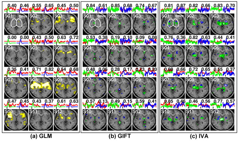
The resulting individual (S01~S12) activation patterns within the thalamus and basal ganglia along with the averaged actual BOLD signals (red), the canonical HRF (green & blue) from GLM, and the estimated TCs (green: thalamus-related & blue: basal ganglia-related) from GIFT and IVA on top of the image plots (a number denotes a correlation coefficient between actual BOLD signal and the canonical HRF or estimated TC). Example activation patterns on a single axial slice (Z=0mm in the MNI space; p<0.01) are shown. An approximate margin of the subcortical areas is marked by a white line.
As an alternative approach on the selection of the number of ICs for the multivariate GIFT and IVA methods, a minimum description length (MDL) algorithm was employed using the GIFT toolbox (Calhoun et al., 2001). The resulting estimated number of ICs was 17 (76.9±14.6% of a sum of the total eigenvalues). In order to find out the performance changes depending on the number of ICs, we also tested for 30 (86.7±10.2%) and 40 (91.6±6.8%) ICs.
III. Results
A. Simulated Data Analysis
The results from the simulated data, along with the layout of the data preparation introduced in the Methods Section, are shown in Fig. 3. Figure 3b illustrates the results from the GLM where the default canonical HRF in SPM2 was used as the reference regressor. Figures 3c and 3d show the estimated task-related TCs and corresponding IC maps across the 12 spatial patterns (simulating different subjects) using GIFT and IVA, as represented in pseudo-colored z-scores. In the figure, blue lines represent the extracted task-related TCs from the activation areas related with trial 1 (with mutually overlapped areas among the subjects) and green lines represent the extracted task-related TCs from the activation areas related to trial 2 (with no overlapped areas among the subjects). Both TCs are overlaid with the modeled HRF (red) in order to show the degree of similarity (a number represents a correlation coefficient).
For GLM (Fig. 3b), since two canonical HRFs corresponding to two assumed trial-based task-paradigm (one trial per activation area) were used as regressors for the simulated data sets, there were two sets of activation maps and time courses. Similarly, for IVA (Fig. 3d), after the non-parametric estimation of both activation areas and time courses, only two output components and out of 55 showed the activation patterns within the assumed activation areas of and , respectively. For GIFT (Fig. 3c), only one of the 55 components ( ) showed the activation patterns corresponding to the activation area modeled by , which represented the activation profiles that completely overlapped among the (modeled) subjects. However, several output components, for example, , and , represented the activation patterns that partially overlapped from the area modeled by .
From the results of GLM, two simulated activation patterns, regardless of the overlapping features, were not readily detected. This type of result was anticipated since the modeled source HRFs with biphasic content significantly deviated from the classical canonical HRF. The situation improved in the results using GIFT, shown in Fig. 3c, whereby the IC maps governed by HRF1 were decomposed as the 54th output for all subjects ( ). On the other hand, the sites of simulated activation in the case of the HRF2 (distributed individual activations in proximity without any overlap) were not decomposed into a single output component, but were distributed over several outputs ( ).
IVA, on the other hand, showed noticeable improvement for detecting modeled biphasic BOLD signals along with activation patterns across the subjects. As shown in Fig 3d, two IC maps ( ) detected activations of the modeled task-related HRF1 and HRF2 within a single output component. Only a few of HRF2-related activation maps, corresponding to subjects 1 and 4 ( ), were not successfully identified whereby subjects 1 and 4 simulated the low BOLD CNR (0.5% and 0.7% respectively). In terms of the ability to extract the modeled HRFs (as indicated by a correlation coefficient), the estimated TCs obtained using IVA showed higher similarity (0.91±0.06) compared to those obtained using GIFT (0.80±0.09).
Figure 4 presents the results from the reduced numbers of ICs estimated from GIFT and IVA. Overall, the GIFT and IVA methods performed similarly whereby each of the two assumed ICs (both activation maps and TCs) were successfully decomposed into the same index of output component across all the subjects. Again, the HRF2-related ICs of the subjects #1 and #4 were underestimated due to the low CNRs. The higher correlation coefficients between the assumed HRFs and estimated time courses were observed from IVA (0.88±0.12) compared to GIFT (0.70±0.16). This is consistent with the findings we observed from analyzing the data using 55 estimated ICs.
Figure 4.
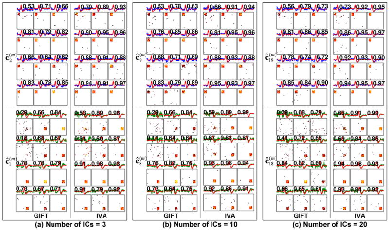
The estimated IC maps and TCs for the reduced numbers of ICs from the GIFT and IVA methods. A figure layout including the used color-coding scheme is identical to that of Fig. 3.
B. fMRI Data Analysis: Individual Activation
The computation time of IVA learning was about 10 hours and memory usage was about 340MB (computer specs: 2.8GHz Intel Pentium 4 Xeon Processor with 3.5GB RAM; 1000 clusters for each iteration; 500 iterations in total; 176,136 voxels within the thresholded brain region in the MNI space).
The estimation results of the 50 ICs of the fMRI data obtained from 12 individuals (S01~S12) are shown in Fig. 5 from a single axial slice (Z=0mm of MNI coordinate) over the thalamus and basal ganglia. The approximate margins of the subcortical areas are marked by a white line. Two averaged BOLD signals of activated voxels (p<0.01) within the thalamus and basal ganglia (red line; not necessarily coming from the same slice as shown) were plotted above each individual activation map. The modeled HRFs (GLM) and estimated TCs (GIFT/IVA) are also shown (green: thalamus & blue: basal ganglia) with an indication of the degree of conformity with respect to the averaged BOLD time series as a correlation coefficient. From the individual processing results based on the univariate GLM approach (Fig 5a), the activation patterns (yellow; p<0.01) showed that there was significant variability across the subjects. For example, there was significant activation across the basal ganglia in S06 whereas there was virtually no activation from S04 and S05.
The results from the GIFT on the extraction of the activation patterns within the subcortical areas are shown in Fig 5b. The estimated TCs (green: thalamus-related & blue: basal ganglia-related) were overlaid on the averaged BOLD time series (red). GIFT performed better than GLM in extracting task-related signals from subcortical areas. For example, non-existing activation from the left thalamus from S01 was subsequently detected using GIFT. Similarly, bilateral activation in the basal ganglia, as is evident from S10 and S11, was not detected from the result obtained using GLM. Compared to the results from GIFT or GLM, the IVA method showed a markedly improved ability in extracting subcortical areas on an individual basis (Fig. 5c) where the activations from the thalamus and putamen were detected from virtually all subjects.
In order to further investigate the difference of HRs within and across subjects as well as across brain regions, the averaged percent BOLD signal of activated voxels from individual activation maps (p<10−3) by GIFT and IVA are represented in Fig. 6 as image plots using the method by Duann et al. (2002). Using this image representation of the BOLD signal (within ±1.5% as a pseudo-colored plot), the differences of BOLD intensities can be readily discriminated. In order to find out the conformity between the averaged BOLD signal and canonical HRF, a correlation coefficient was calculated and is shown with each time plot.
Figure 6.

The image plots of the averaged percent BOLD signals (truncated within ±1.5%) of activated areas (p<10−3) of the estimated IC map for each subject. The BOLD image plots corresponding to the primary motor-area (cortical region) from a motor-related IC map from GIFT and IVA is shown to compare the BOLD image plots corresponding to the thalamus and basal ganglia (subcortical region). A task-related response is marked as a black box and example variations from the hypothesized HRF are indicated with arrows. In the bottom of each image plot, the canonical HRF from GLM (green) and an averaged percent (%) BOLD signal (red) along with standard deviation (blue) across all subjects are shown as temporal plots (a number denotes a correlation coefficient between the canonical HRF and averaged BOLD signal).
The BOLD measurement from the primary motor-area was in good agreement with the hypothesized HRF. Compared to GIFT, the averaged BOLD signal across the subjects within the activated areas by IVA showed a higher correlation with the hypothesized HRF (i.e. 0.70 by GIFT vs. 0.88 by IVA), as was also visible by more concentrated task-related activity during the task period (marked as a black box). BOLD signal within the thalamus and basal ganglia deviated from the cortex-based canonical HRF, and showed significant variations across the subjects and regions (as indicated with arrows). As anticipated, the correlation coefficients between the averaged BOLD signal and the canonical HRF measured within these areas were less than CCs measured in the motor-area (i.e. 0.55 & 0.63 by GIFT and 0.68 & 0.49 by IVA). This was due to relatively low signal contrast and biphasic/high-frequency BOLD characteristics within the subcortical area compared to the cortical area. These results may indicate the efficacy and utility of the non-parametric and multivariate approaches in the detection of the atypical BOLD responses compared to the parametric and univariate approaches. Both GIFT and IVA successfully detected the regions showing the HRs that deviate from the canonical HRF.
C. fMRI Data Analysis: Group Inference
After the identification of individual activation patterns, the group inference results based on RFX is shown in Fig. 7. Two different threshold values (p<10−3 & p<10−5) were applied for each RFX-based group activation map and activation patterns were also pseudo-colored (thalamus in green and basal ganglia in blue). The range of axial slices shown covers from Z=0mm to 12mm with a step of 4mm.
Figure 7.

The resulting group activation trend obtained from RFX within several axial slices (Z=0, 4, 8, & 12mm in the MNI space) is shown for different p-values (p<10−3 & p<10−5) in order to compare the statistical significance of the analyzed activations depending on the employed method. The labeled anatomical information of the activation loci is summarized in Table 1.
From visual inspection of the results, GLM detected the bilateral activation in the thalamus from Z=0mm (p<10−3) and the unilateral thalamic activation at a slightly superior slice, at Z=4mm (p<10−3). However, the activation within the basal ganglia was not detected. GIFT, on the other hand, detected the putamen activation in the lentiform nucleus bilaterally in the slice Z=0 and 4mm (p<10−3). However, the thalamic activation was grossly distorted with adjacent ventricles. Again, for the higher threshold level of p<10−5, many of the activations were missed in the results from GIFT. The bilateral activation in the posterior superior temporal gyri (shown in Z=4~12mm) from GLM, showing a classical HRF pattern, was excluded from further RFX analysis of the corresponding IC maps by GIFT and IVA in order to target subcortical areas. In order to ensure that subcortical activation was not missed during the course of manual selection, different IC maps were searched again for possible definition, but without any apparent improvement.
The localized group activation areas identified by IVA showed substantially higher z-scores that remained even for the very stringent threshold condition of p<10−5. The location and the size of activation identified from each of the group-processing methods are summarized in Table. 1. Notably, the distinct activation within the anterior putamen and ventral posterolateral/mediodorsal thalamus only identified through IVA were well matched with the motor control circuitry within subcortical areas, whereby these areas are known to be associated with movement parameters such as complexity and frequency (Lehericy et al., 2006). Interestingly, as is evident from slice Z=4mm, the IVA method was able to identify the thalamic activation revealed only by GLM and the putamen activation revealed only by GIFT, suggesting the ability to detect the areas that could be missed by using either GLM or GIFT alone.
Figure 8 shows the RFX-based group activation maps corresponding to the reduced numbers of ICs (the location and size of activation loci were summarized in Table 2). The activation patterns within the thalamus and basal ganglia were now decomposed into one output component due the reduced number of ICs (except for GIFT analysis using 40 estimated ICs). Although the overall results are consistent with those obtained from the 50 estimated ICs, it is interesting to note that the activation patterns from the 17 ICs (smallest number of ICs) using GIFT showed strongest statistical significance compared to those from the 30 and 40 ICs. On the other hand, IVA tends to show reduced level of statistical significance from the results obtained from using 17 ICs.
Figure 8.
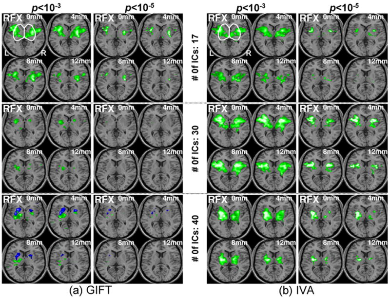
The RFX-based group activation trend within subcortical areas from GIFT and IVA is shown for several cases of the reduced numbers of estimated ICs (i.e. 17, 30, & 40) and for two different p-values. The reduced number 17 was estimated using the MDL tool available in the GIFT toolbox. The labeled anatomical information of the activation loci is summarized in Table 2.
Table 2.
Cortical regions of the group activation maps corresponding to Fig. 8 (thresholded at p<10−5 with clusters greater than 5 voxels using SPM2). Notations used are same as those in Table 1.
| Region | Side | Cluster Size | x | y | z | Peak z-score | |
|---|---|---|---|---|---|---|---|
| Number of Estimated ICs: 17 | |||||||
| GIFT | LN/Put. | R | 862 | 32 | −16 | 8 | 6.68 |
| “ | “ | 34 | −10 | −6 | 5.51 | ||
| “ | “ | 30 | −2 | 4 | 5.41 | ||
| LN/Put. | L | 915 | −34 | 6 | 4 | 5.66 | |
| LN/Put./LGP/MGP | “ | −25 | −12 | −8 | 5.25 | ||
| Thal. | R | 26 | 8 | −26 | 4 | 4.89 | |
|
| |||||||
| IVA | LN/Put. | L | 717 | −32 | 4 | 0 | 5.34 |
| “ | “ | −30 | 14 | −5 | 5.07 | ||
| LN/Put./Claustrum/Insula | R | 521 | 35 | −12 | −4 | 5.27 | |
| LN/Put./Thal./VPLN/LPN/VLN | “ | 257 | 24 | −16 | 8 | 5.15 | |
| Insula/LN/Put. | “ | 32 | −20 | 8 | 5.07 | ||
| Thal./MDN | L | 19 | −6 | −22 | 0 | 4.73 | |
| Insular/LN/Put. | “ | 8 | −34 | −20 | 12 | 4.46 | |
|
| |||||||
| Number of Estimated ICs: 30 | |||||||
| GIFT | LN/Put. | L | 32 | −32 | 0 | 2 | 4.75 |
| LN/Put./LGP/Thal./VAN | “ | 6 | −20 | −4 | 10 | 4.54 | |
|
| |||||||
| IVA | LN/Put./Claustrum/Insula | R | 2067 | 30 | 6 | 6 | 6.30 |
| Claustrum/LN/Put./Insula | “ | 35 | −10 | −5 | 5.70 | ||
| LN/Put./Claustrum/Insula | L | 2644 | −32 | 4 | 6 | 6.28 | |
| Claustrum/LN/Put./Insular | “ | −30 | 18 | −2 | 5.98 | ||
|
| |||||||
| Number of Estimated ICs: 40 | |||||||
| GIFT | Thal./VLN/VAN/LN/MGP | L | 43 | −14 | −8 | 0 | 5.13 |
| Thal./VAN/VLN/MDN | “ | −5 | −5 | −4 | 4.58 | ||
| LN/Put./Claustrum | “ | 51 | −32 | −22 | 0 | 5.05 | |
| “ | R | 8 | 32 | −6 | −14 | 5.01 | |
| Caudate | L | 9 | −32 | −34 | 8 | 4.73 | |
| LN/LGP | R | 12 | 28 | −6 | −2 | 4.69 | |
|
| |||||||
| LN/Put. | L | 356 | −22 | 12 | −4 | 5.78 | |
| “ | “ | −30 | −2 | −4 | 5.40 | ||
| “ | “ | −24 | 8 | 8 | 4.80 | ||
| “ | R | 24 | 24 | 10 | 4 | 4.89 | |
| LN/Put./LGP | L | 5 | −30 | −14 | 2 | 4.37 | |
|
| |||||||
| IVA | LN/Put./LGP | L | 1879 | −26 | −2 | 2 | 6.49 |
| “ | “ | −28 | −12 | 5 | 5.42 | ||
| Thal./VLN/VAN | “ | −18 | −10 | 12 | 5.81 | ||
| Thal./VLN/VAN/LN | R | 595 | 16 | −8 | 10 | 5.71 | |
| LN/Put./Claustrum/Insula | “ | 32 | 5 | 2 | 5.25 | ||
| Thal./VPLN/VPMN/VLN/LGP | “ | 18 | −15 | 0 | 5.13 | ||
| LN/Put. | L | 11 | −24 | 16 | 4 | 4.47 | |
LN: Lentiform Nucleus; Put.: Putamen; LGP: Lateral Globus Pallidus; MGP.: Medial Globus Pallidus; Thal.: Thalamus; VPLN.: Ventral Posterior Lateral Nucleus; VPMN: Ventral Posterior Medial Nucleus; LPN: Lateral Posterior Nucleus; VLN: Ventral Lateral Nucleus; VAN: Ventral Anterior Nucleus; MDN: Medial Dorsal Nucleus.
IV. Discussion
Group fMRI processing of subcortical areas is particularly challenging since the amount of BOLD signal contrast generated by these areas is typically smaller compared to those from other parts of the brain. The reduced CNR is compounded by the BOLD signals that are inconsistent across the subjects and from the typical canonical HRFs. In this study, we proposed a novel multivariate method for the processing of group fMRI data using IVA, targeting the group-trend extraction of small activation patterns from subcortical areas. Based on the analysis of the simulated data, the IVA algorithm successfully characterized group trends in activation patterns that are slightly shifted in space while conventional group processing methods were not able to do so. Also, IVA, as one of blind-source-separation (BBS) techniques, was able to detect the locations with hemodynamic responses that do not follow the modeled canonical HRFs. In contrast to conventional ICA-based group processing, IVA derived the spatially-similar trend in activation across subjects as a single output vector component.
From the analysis of the actual fMRI data, IVA also demonstrated superior utility in extracting small subcortical activations from the thalamus/basal ganglia activation during the motor task, compared to GLM or GIFT. Unlike GIFT, which still requires a degree of manual intervention or a heuristic data reduction scheme from individual to group data, IVA inherently extracted the common spatial features of activation patterns across the subjects into a single vector component. Therefore, the level of statistical significance in the group activation map dramatically increased since the IVA algorithm can extract each individual’s activation patterns that are mutually dependent on the spatial domain across the subjects. The inherent spatial homogeneity of the estimates from the GIFT can be traced to the PCA-based dimension reduction scheme across all the subjects’ data whereby the estimation of time courses is likely to be biased towards the temporal characteristics from the commonly activated voxels across all the subjects. More detailed explanation on the inherent restriction of the GIFT is described elsewhere (Esposito et al., 2005; Beckmann and Smith, 2005; Lee et al., 2008).
As further demonstrated from the averaged BOLD signal of fMRI data during the right hand motor task (Fig. 6), BOLD signal measured from the thalamus and basal ganglia, including the putamen, deviated from the canonical HRF (green) and had large inter-subject variations (in arrows). On the other hand, BOLD signal from the primary somatomotor areas (left precentral gyrus) was similar to the modeled HRF. This confirmed the observation that the deviating characteristics of the BOLD signal arising from the subcortical areas are known as main difficulties in detecting the corresponding neural activities by using the conventional cortex-based reference HRF model (Moritz et al., 2000; Riecker et al., 2006).
In addition to the ability to characterize BOLD signal patterns that depart from the canonical model, IVA also markedly elevated the group-level statistical significance among the three tested methods. For example, with just a short data acquisition for a single trial (65-sec), the group activation derived from IVA survived the threshold level of p<10−5 while most of the activation from the GLM or GIFT at this threshold condition escaped from being detected. This markedly increased statistical significance can be appreciated from the individual results (Fig. 5). Individual activation maps processed by GLM or GIFT showed large inter-subject variability. However, IVA was able to extract strikingly consistent and similar activation patterns across the subjects. Another advantage of IVA, compared to the ICA-based approach, is that output component maps which are automatically grouped across subjects already reflect the group trend. Therefore, the IVA method does not involve the complicated selection criteria that are necessary for the ICA-based methods. As demonstrated in Fig. 3c, the sites of simulated activation (individual activation distributed in proximity without any overlap) were not decomposed in a single output component, but rather distributed over several outputs.
Meanwhile, the performance from the GIFT method appears to be more sensitive to the number of estimated ICs than that of the IVA method whereby the results from the smaller number of ICs (Figs. 4 & 8) provided more accurate (for simulated data) and statistically significant (for real data) compared to those based on using more ICs (Figs. 3 & 7). On the other hand, for IVA, the slight degradation of the statistical significance observed for the smaller number of ICs (i.e. 17; Fig. 8b) may be due to the inhomogeneous level of BOLD contrast within the subcortical areas among the subjects. It suggests that IVA may be susceptible to excessive reduction in ICs. Tensorial ICA, as an extension of ICA algorithm (Beckmann and Smith, 2005; Lee et al., 2008), may be used to complement the ICA-based analysis as well as the IVA scheme.
Many cognitive studies have been plagued with potential underestimation of the detection from the subcortical regions due to spatial smoothing and correction schemes. IVA, therefore, could be gainfully applied to the studies whereby group activation is needed for the small activation loci or the area that shows small BOLD contrast. Neuro-psychiatric fMRI studies, in which the activation could be altered by the underlying pathology or the crucial neural circuitries that are often involved in small areas, can benefit from the IVA approach. Schizophrenia, for example, involves abnormal activation patterns as well as anatomical morphology across the brain. Recent studies indicated that aberrant cognitive and emotional behavior shown among schizophrenic persons can be traced to the activation patterns that differ from healthy controls (Aleman and Kahn, 2005; Holt et al., 2006; Harrison et al., 2007). fMRI has been actively used to study these differences. However, the results were mostly based on the GLM-based approaches. IVA, in this context, may be used to detect differences in group trends that have been evading detection based on the conventional approaches. It is important to note that the proposed IVA method may be effective in analyses of fMRI data that are susceptible to atypical BOLD signals among the subjects and brain areas (in terms of magnitude, duration, and timing of onsets). This applies to the analysis of, for example, data obtained from individuals with neuroleptic medications (Eyler et al., 2004; Fahim et al., 2005; Ford et al., 2005) or substance abuse (Gollub et al., 1998; Lee et al., 2003; Chang et al., 2006; Van Horn et al., 2006).
The future utility of the IVA method can be also appreciated from the stand point of functional connectivity analysis during the resting state. Recently, several fMRI works have revealed that there are inherent functional connections established among different neural substrates that share the similar hemodynamic trend without the presence of an apparent task (Castellanos et al., 2007; Wang et al., 2007). The study on this resting state without any apparent stimulation or task, therefore, can not be studied using model-driven approaches. IVA, with its ability to sort out the similar spatio-temporal features across subjects, can help elucidate the connectivity across the neural activation during the resting state.
The current IVA-based approach is achieved at the cost of more extensive computational demands, compared to the existing GLM or ICA-based methods. This is because an individual unmixing matrix is iteratively trained using the results from other subjects (represented as the nonlinear function, ϕ(ĉ(m) (v)) of Eq. (6), which subsequently requires the updates of all the unmixing matrices in parallel. The increased computational load associated with IVA can be alleviated by increasing the capacity of computer memory or utilization of a multi-core CPU. Although the current study shows the potential utility of IVA, elaborate sets of optimization processes would be needed in terms of learning parameters and selecting components-of-interest for the fully-automated group processing. The application of the IVA method to analyze fMRI data examining the various types of neuropsychiatric disorders would constitute future areas of study.
Table 1.
Cortical regions of the group activation maps (thresholded at p<10−5 with clusters greater than 5 voxels using SPM2). Notation used for the side of activation; L-Left & R-Right. The center of a cluster (x, y, & z; in mm) is represented in the MNI space.
| Region | Side | Cluster Size | x | y | z | Peak z-score | |
|---|---|---|---|---|---|---|---|
| GLM | Thalamus: Ventral Lateral Nucleus | L | 16 | −12 | −12 | −2 | 4.59 |
| “: Subthalamic Nucleus | R | 7 | 16 | −12 | −4 | 4.44 | |
| “: Extra Nuclear | L | 7 | −24 | −24 | 2 | 4.37 | |
|
| |||||||
| GIFT | Sub-lobar: Lateral Ventricle | L | 307 | −2 | 0 | 10 | 5.49 |
| “ | R | 5 | 2 | 16 | 4.73 | ||
| Thalamus: Extra Nuclear | L | 44 | −6 | −20 | 16 | 5.23 | |
|
| |||||||
| Lentiform Nucleus: Putamen | L | 22 | −18 | 14 | −4 | 5.25 | |
| “ | R | 96 | 24 | −4 | 4 | 5.25 | |
|
| |||||||
| IVA | Thalamus: Ventral Lateral/Anterior Nucleus | R | 295 | 16 | −8 | 10 | 5.65 |
| “: Ventral Lateral Nucleus | R | 20 | −16 | 14 | 5.51 | ||
| “: Medial Dorsal/Midline/Anterior Nucleus | R | 8 | −16 | 12 | 5.02 | ||
| “: Ventral Posterior Lateral/Medial Nucleus | L | 1030 | −18 | −16 | 2 | 5.63 | |
| “: Medial Dorsal Nucleus | L | −8 | −14 | 6 | 5.44 | ||
| Lentiform Nucleus: Putamen | L | −28 | 0 | 2 | 5.39 | ||
| Sub-lobar: Extra Nuclear | R | 83 | 36 | −14 | 0 | 5.08 | |
| Lentiform Nucleus: Putamen | R | 32 | 0 | −2 | 4.28 | ||
| Thalamus: Extra Nuclear | R | 37 | 26 | −32 | 4 | 4.91 | |
| “ | R | 9 | 12 | −6 | −6 | 4.45 | |
|
| |||||||
| Lentiform Nucleus: Putamen | L | 462 | −28 | 4 | 2 | 5.89 | |
| “ | L | −18 | 12 | −8 | 4.92 | ||
| Lentiform Nucleus: Putamen | R | 344 | 26 | 6 | −2 | 5.50 | |
| “ | R | 26 | −4 | 2 | 5.43 | ||
Acknowledgments
This work was partially supported in part by grants from NIH (R01-NS048242 to Yoo, SS and NIH U41RR019703 to Jolesz), the Korean Ministry of Commerce, Industry, and Energy (grant No. 2004-02012 to S.S. Yoo), and Gachon Neuroscience Research Institute Grant (to Yoo SS). Authors thank the editorial assistance of Mr. Matthew Marzelli.
References
- Aguirre GK, Zarahn E, D’Esposito M. The variability of human. BOLD hemodynamic responses. NeuroImage. 1998;8:360–369. doi: 10.1006/nimg.1998.0369. [DOI] [PubMed] [Google Scholar]
- Aleman A, Kahn RS. Strange feelings: do amygdala abnormalities dysregulate the emotional brain in schizophrenia? Prog Neurobiol. 2005;77:283–298. doi: 10.1016/j.pneurobio.2005.11.005. [DOI] [PubMed] [Google Scholar]
- Bandettini PA, Jesmanowicz A, Wong EC, Hyde JS. Processing strategies for time-course data sets in functional MRI of the human brain. Magn Reson Med. 1993;30:161–173. doi: 10.1002/mrm.1910300204. [DOI] [PubMed] [Google Scholar]
- Beckmann C, Smith S. Tensorial extensions of independent component analysis for multisubject FMRI analysis. Neuroimage. 2005;25:294–311. doi: 10.1016/j.neuroimage.2004.10.043. [DOI] [PubMed] [Google Scholar]
- Calhoun VD, Adali T, Pearlson GD, Pekar JJ. A method for making group inferences from functional MRI data using independent component analysis. Hum Brain Mapp. 2001;14:140–151. doi: 10.1002/hbm.1048. [DOI] [PMC free article] [PubMed] [Google Scholar]
- Castellanos FX, Margulies DS, Kelly C, Uddin LQ, Ghaffari M, Kirsch A, Shaw D, Shehzad Z, Di Martino A, Biswal B, Sonuga-Barke EJ, Rotrosen J, Adler LA, Milham MP. Cingulate-Precuneus Interactions: A New Locus of Dysfunction in Adult Attention-Deficit/Hyperactivity Disorder. Biol Psychiatry. 2008;63:332–337. doi: 10.1016/j.biopsych.2007.06.025. [DOI] [PMC free article] [PubMed] [Google Scholar]
- Chang L, Yakupov R, Cloak C, Ernst T. Marijuana use is associated with a reorganized visual-attention network and cerebellar hypoactivation. Brain. 2006;129:1096–1112. doi: 10.1093/brain/awl064. [DOI] [PubMed] [Google Scholar]
- Cichocki A, Amari S. Adaptive blind signal and image processing: Learning algorithms and applications. John Wiley & sons, Ltd; West Sussex: 2002. [Google Scholar]
- Duann JR, Jung TP, Kuo WJ, Yeh TC, Makeig S, Hsieh JC, Sejnowski TJ. Single-trial variability in event-related BOLD signals. Neuroimage. 2002;15:823–835. doi: 10.1006/nimg.2001.1049. [DOI] [PubMed] [Google Scholar]
- Esposito F, Scarabino T, Hyvarinen A, Himberg J, Formisano E, Comani S, Tedeschi G, Goebel R, Seifritz E, Di Salle F. Independent component analysis of fMRI group studies by self-organizing clustering. Neuroimage. 2005;25:193–205. doi: 10.1016/j.neuroimage.2004.10.042. [DOI] [PubMed] [Google Scholar]
- Esposito F, Di Salle F, Hennel F, Santopaolo O, Herdener M, Scheffler K, Goebel R, Seifritz E. A multivariate approach for processing magnetization effects in triggered event-related functional magnetic resonance imaging time series. Neuroimge. 2006;30:136–143. doi: 10.1016/j.neuroimage.2005.09.012. [DOI] [PubMed] [Google Scholar]
- Eyler LT, Olsen RK, Jeste DV, Brown GG. Abnormal brain response of chronic schizophrenia patients despite normal performance during a visual vigilance task. Psychiatry Res. 2004;130:245–57. doi: 10.1016/j.pscychresns.2004.01.003. [DOI] [PubMed] [Google Scholar]
- Fahim C, Stip E, Mancini-Marie A, Gendron A, Mensour B, Beauregard M. Differential hemodynamic brain activity in schizophrenia patients with blunted affect during quetiapine treatment. J Clin Psychopharmacol. 2005;25:367–71. doi: 10.1097/01.jcp.0000168880.10793.ed. [DOI] [PubMed] [Google Scholar]
- Ford JM, Johnson MB, Whitfield SL, Faustman WO, Mathalon DH. Delayed hemodynamic responses in schizophrenia. Neuroimage. 2005;26:922–931. doi: 10.1016/j.neuroimage.2005.03.001. [DOI] [PubMed] [Google Scholar]
- Friston KJ, Holmes AP, Worsley KJ. How many subjects constitute a study? Neuroimage. 1999;10:1–5. doi: 10.1006/nimg.1999.0439. [DOI] [PubMed] [Google Scholar]
- Gollub RL, Breiter HC, Kantor H, Kennedy D, Gastfriend D, Mathew RT, Makris N, Guimaraes A, Riorden J, Campbell T, Foley M, Hyman SE, Rosen B, Weisskoff R. Cocaine decreases cortical cerebral blood flow but does not obscure regional activation in functional magnetic resonance imaging in human subjects. J Cereb Blood Flow Metab. 1998;18:724–734. doi: 10.1097/00004647-199807000-00003. [DOI] [PubMed] [Google Scholar]
- Gur RC, Turetsky BI, Loughead J, Waxman J, Snyder W, Ragland JD, Elliott MA, Bilker WB, Arnold SE, Gur RE. Hemodynamic responses in neural circuitries for detection of visual target and novelty: An event-related fMRI study. Hum Brain Mapp. 2007;28:263–274. doi: 10.1002/hbm.20319. [DOI] [PMC free article] [PubMed] [Google Scholar]
- Handwerker DA, Ollinger JM, D’Esposito M. Variation of BOLD hemodynamic responses across subjects and brain regions and their effects on statistical analyses. Neuroimage. 2004;21:1639–1651. doi: 10.1016/j.neuroimage.2003.11.029. [DOI] [PubMed] [Google Scholar]
- Harrison BJ, Yücel M, Pujol J, Pantelis C. Task-induced deactivation of midline cortical regions in schizophrenia assessed with fMRI. Schizophr Res. 2007;91:82–86. doi: 10.1016/j.schres.2006.12.027. [DOI] [PubMed] [Google Scholar]
- Holt DJ, Kunkel L, Weiss AP, Goff DC, Wright CI, Shin LM, Rauch SL, Hootnick J, Heckers S. Increased medial temporal lobe activation during the passive viewing of emotional and neutral facial expressions in schizophrenia. Schizophr Res. 2006;82:153–162. doi: 10.1016/j.schres.2005.09.021. [DOI] [PubMed] [Google Scholar]
- Kim T, Attias HT, Lee SY, Lee TW. Blind source separation exploiting higher-order frequency dependencies. IEEE Trans Audio Speech and Language Process. 2007;15:70–79. [Google Scholar]
- Lehericy S, Bardinet E, Tremblay L, Van de Moortele PF, Pochon JB, Dormont D, Kim DS, Yelnik J, Ugurbil K. Motor control in basal ganglia circuitries using fMRI and brain atlas approaches. Cereb Cortex. 2006;16:149–161. doi: 10.1093/cercor/bhi089. [DOI] [PubMed] [Google Scholar]
- Lee JH, Telang FW, Springer CS, Jr, Volkow ND. Abnormal brain activation to visual stimulation in cocaine abusers. Life Sci. 2003;73:1953–1961. doi: 10.1016/s0024-3205(03)00548-4. [DOI] [PubMed] [Google Scholar]
- Lee JH, Lee TW, Jolesz FA, Yoo SS. Independent vector analysis IVA: Multivariate approach for fMRI group study. Neuroimage. 2008;40:86–109. doi: 10.1016/j.neuroimage.2007.11.019. [DOI] [PubMed] [Google Scholar]
- Lowe MJ, Lurito JT, Mathews VP, Phillips MD, Hutchins GD. Quantitative comparison of functional contrast from BOLD-weighted spin-echo and gradient-echo echo planar imaging at 1.5 Tesla and H2 15O PET in the whole brain. J Cereb Blood Flow Metab. 2000;20:1331–1340. doi: 10.1097/00004647-200009000-00008. [DOI] [PubMed] [Google Scholar]
- McGonigle DJ, Howseman AM, Athwal BS, Friston KJ, Frackowiak RS, Holmes AP. Variability in fMRI: an examination of intersession differences. NeuroImage. 2000;11:708–734. doi: 10.1006/nimg.2000.0562. [DOI] [PubMed] [Google Scholar]
- McKeown MJ, Makeig S, Brown GG, Jung TP, Kindermann SS, Bell AJ, Sejnowski TJ. Analysis of fMRI data by blind separation into independent spatial components. Hum Brain Mapp. 1998;6:160–188. doi: 10.1002/(SICI)1097-0193(1998)6:3<160::AID-HBM5>3.0.CO;2-1. [DOI] [PMC free article] [PubMed] [Google Scholar]
- Meltzer JA, Negishi M, Constable RT. Biphasic hemodynamic responses influence deactivation and may mask activation in block-design fMRI paradigms. Hum Brain Mapp. 2007 Apr 20; doi: 10.1002/hbm.20391. [Epub ahead of print] [DOI] [PMC free article] [PubMed] [Google Scholar]
- Moritz CH, Meyerand ME, Cordes D, Haughton VM. Functional MRI imaging activation after finger tapping has a shorter duration in the basal ganglia than in the sensorimotor cortex. AJNR Am J Neuroradiol. 2000;21:1228–1234. [PMC free article] [PubMed] [Google Scholar]
- Peterson BS, Skudlarski P, Gatenby JC, Zhang H, Anderson AW, Gore JC. An fMRI study of Stroop word-color interference: evidence for cingulate subregions subserving multiple distributed attentional systems. Biol Psychiatry. 1999;25:1237–1258. doi: 10.1016/s0006-3223(99)00056-6. [DOI] [PubMed] [Google Scholar]
- Riecker A, Kassubek J, Gröschel K, Grodd W, Ackermann H. The cerebral control of speech tempo: opposite relationship between speaking rate and BOLD signal changes at striatal and cerebellar structures. Neuroimage. 2006;29:46–53. doi: 10.1016/j.neuroimage.2005.03.046. [DOI] [PubMed] [Google Scholar]
- Scholz VH, Flaherty AW, Kraft E, Keltner JR, Kwong KK, Chen YI, Rosen BR, Jenkins BG. Laterality, somatotopy and reproducibility of the basal ganglia and motor cortex during motor tasks. Brain Res. 2000;879:204–215. doi: 10.1016/s0006-8993(00)02749-9. [DOI] [PubMed] [Google Scholar]
- Svensen M, Kruggel F, Benali H. ICA of fMRI group study data. Neuroimage. 2002;16:551–563. doi: 10.1006/nimg.2002.1122. [DOI] [PubMed] [Google Scholar]
- Van Horn JD, Yanos M, Schmitt PJ, Grafton ST. Alcohol-induced suppression of BOLD activity during goal-directed visuomotor performance. Neuroimage. 2006;31:1209–1221. doi: 10.1016/j.neuroimage.2006.01.020. [DOI] [PubMed] [Google Scholar]
- Wang K, Liang M, Wang L, Tian L, Zhang X, Li K, Jiang T. Altered functional connectivity in early Alzheimer’s disease: A resting-state fMRI study. Hum Brain Mapp. 2007;28:967–978. doi: 10.1002/hbm.20324. [DOI] [PMC free article] [PubMed] [Google Scholar]
- Worsley KJ, Friston KJ. Analysis of fMRI time-series revisited—again. Neuroimage. 1995;2:173–181. doi: 10.1006/nimg.1995.1023. [DOI] [PubMed] [Google Scholar]