A Robust Algorithm for Point Set Registration Using Mixture of Gaussians

Abstract

This paper proposes a novel and robust approach to the point set registration problem in the presence of large amounts of noise and outliers. Each of the point sets is represented by a mixture of Gaussians and the point set registration is treated as a problem of aligning the two mixtures. We derive a closed-form expression for the L₂ distance between two Gaussian mixtures, which in turn leads to a computationally efficient registration algorithm. This new algorithm has an intuitive interpretation, is simple to implement and exhibits inherent statistical robustness. Experimental results indicate that our algorithm achieves very good performance in terms of both robustness and accuracy.

1. Introduction

Point set representations of image data, e.g., feature points, are commonly used in many applications and the problem of registering point-sets frequently arises in a variety of these application domains. Extensive studies on the point set registration and related problems can be found in a rich literature covering both theoretical and practical issues relating to computer vision and pattern recognition.

Let M,the model set of size n_M and S, the scene set of size n_S be two point-sets belonging to a finite-dimensional real vector space R^d. The task of point pattern matching or point-set registration is either to establish a consistent point-to-point correspondence between two sets or to recover the spatial transformation which yields the best alignment.

The iterative closest point (ICP) algorithm is one of most common approaches to feature-based image registration and shape matching problem because of its simplicity and performance. Nonetheless, it has its own limitations. The non-differentiable cost function associated with ICP introduces the local convergence problem which requires sufficient overlap between the data-sets and a close initialization. Also, a naive implementation of ICP is know to be prone to outliers which prompted several more robust variations [1, 2]. Another elegant method is the partial Hausdorff distance registration [3] which incorporates an underlying robust mechanism similar to the least median of squares (LMedS) technique in robust regression. However, its dependence on a single critical point makes it sensitive to noise and the max of the min approach in the definition is not suitable for performing numerical optimization.

Several significant articles on robust and non-rigid point set matching have been published by Rangaranjan and collaborators [4, 5, 6]. The main strength of their work is the ability to jointly determine the correspondences and non-rigid transformation between two point sets using deterministic annealing and soft-assign. However, in their work, the stability of the registration result is not guaranteed in the case of data with outliers, and hence a good stopping criterion is required. Other related work reported in literature includes [7] where the outliers need to be excluded from the shape context computation.

Another interesting class involves methods that align two point sets without establishing the explicit point correspondence, and thus achieve more robustness to the missing correspondences and outliers. The idea is to model each of the two point sets by a kernel density function and then quantify the (dis)similarity between them using an information-theoretic measure. This (dis)similarity is optimized over a space of coordinate transformations yielding the desired transformation. For instance, Tsin and Kanade [8] propose a kernel correlation based point set registration approach where the cost function is proportional to the correlation of two kernel density estimates. In this paper, we present a method that belongs to the aforementioned class of approaches. We will present the relationship and differences between ours and others’ methods in the next section. The main contributions of our paper are: (i) We suggest the idea of using Gaussian mixture models as a natural and simple way to represent the given point sets. Then, we treat the problem of point set registration as that of aligning two Gaussian mixtures. Interestingly, it turns out that both the iterative closest point (ICP) method [9] and the kernel correlation-based (KC) approach [8] can be interpreted in this framework. (ii) A closed-form expression for the L₂ distance between two Gaussian mixtures is derived, which in turn leads to a computationally efficient registration algorithm. Our new registration algorithm has an intuitive interpretation, is simple to implement and exhibits inherent statistical robustness.

Rest of this paper is organized as follows: in Section 2, we present the main idea of matching point sets using a mixture model representation and show the relationship with ICP and KC methods. Section 3 describes the registration algorithms for rigid and non-rigid transformations. Experimental results with both synthetic data and real data as well as comparisons with other methods are presented in section 4. Finally, conclusions are drawn in Section 5.

2. Mixture Models & Point Matching

The main idea of our technique is, to measure the similarity between two finite point sets by considering their continuous approximations. In this context, one can relate a point set to a probability density function. Considering the point set as a collection of Dirac Delta functions, it is natural to think of a finite mixture model as representation of a point set. As the most frequently used mixture model, a Gaussian mixture is defined as a convex combination of Gaussian component densities ϕ(x|μ_i,Σ_i), where μ_i is the mean vector and Σ_i is the covariance matrix. The probability density function is explicitly given as $p\left(\mathbf{x}\right)={\Sigma }_{i=1}^k{w}_i\varphi (\mathbf{x}\mid {\mu }_i,{\Sigma }_i)$ where w_i are weights associated with the components. If the number of components, k, is quite large, then almost any density may be well approximated by this model. In this paper, we use the Gaussian mixture model to represent the point set explicitly. In a simplified setting, the number of components is the number of the points in the set. And for each component, the mean vector is given by the location of each point. Without prior information, we can assume each component has same weight and each Gaussian is spherical i.e. the covariance is proportional to identity matrix. If the the orientation and anisotropy information are available, the shape and orientation of the covariance matrix can be determined accordingly. For example, when the point set is acquired from an intensity image, additional information can be obtained from the gradient vectors. For a dense point cloud, a mixture model-based clustering or grouping may be performed as a preprocessing procedure.

Recent work on point matching using Gaussian mixture models has been proposed by Chui and Rangarajan [10]; they choose one sparsely distributed point-set as the template density modeled by a Gaussian mixture and treat another relatively dense point-set as sample data. Then the point matching is re-interpreted as a mixture density estimation problem and solved in an EM-like fashion. Instead of the asymmetric point matching case in [10], we treat the problem using mixtures in a symmetrical manner. In this way, the two point-sets, model and scene, are represented by two mixtures of Gaussians. Intuitively, if these two point sets are aligned properly enough, the two resulting mixtures should be statistically similar to each other. Consequently, this raises the key problem: How to measure the similarity/closeness between two Gaussian mixtures?

2.1. L₂ Distance between Gaussian Mixtures

Many measures have been proposed to quantify the similarity between two arbitrary probability distributions. Here we suggest the L₂ distance for measuring similarity between Gaussian mixtures because: (1) The L₂ distance is strongly related to the inherently robust estimator L₂E [11]; (2) There is a closed-form expression for the L₂ distance between Gaussian mixtures, which in turn permits efficient implementation of the registration algorithm.

First, to show the robustness property of the L₂ distance, we start with the density power divergence, a family of divergence measures introduced in Basu et al. [12].

Density Power Divergence

Let f and g be density functions, define the divergence d_α(f, g) to be

$$d_{\alpha }(f,g)=\int \left\{\frac{1}{\alpha }{f}^{1+\alpha }-(1+\frac{1}{\alpha }f{g}^{\alpha })+g^{1+\alpha }\right\}\mathit{dz}$$ (1)

In the case of α → 0, we have, d₀(f, g) = lim_α→₀ d_α(f, g)= ∫ f(z)log{f(z)/g(z)} which gives the well known Kullback-Leibler (KL) divergence. And the minimizer corresponds to maximum likelihood estimation (MLE). On the [integraltext] other hand, when α = 1, the divergence d₁(f, g) = ∫ {f(z) — g(z)}²dz becomes exactly the L₂ distance between the densities, and the corresponding estimator is called L₂E estimator. For general 0 < α < 1, the class of density power divergences provides a smooth bridge between the KL divergence and the L₂ distance. Furthermore, this single parameter α controls the trade-off between robustness and asymptotic efficiency of the parameter estimators which are the minimizers of this family of divergences. The fact that the L₂E is inherently superior to MLE in terms of robustness can be well explained by viewing the minimum density power divergence estimators as a particular case of M-estimators [13]. For in-depth discussion on this issue, we refer the reader to [11].

Next, one can easily derive the closed-form expression for the L₂ distance between two mixtures of Gaussians by noting the formula: ∫ ϕ(x|μ₁, Σ₁)ϕ(x|μ₂, Σ₂) dx = ϕ (0|μ₁—μ₂, Σ₁ + Σ₂). We emphasize the fact that equation (1) does not have a closed form for 0 < α < 2 except for the L₂ distance at α = 1. Hence, this affords an advantage to the L₂ distance since we do not need the numerical integration or approximation which is a practical limitation not only in computation time but also for obtaining sufficient accuracy to perform numerical optimization.

2.2. Related Work

In contrast to the closed-form expression for the L₂ distance between mixtures, there is no such one for the KL divergence between two Gaussian mixtures. In the context of image retrieval, several approaches to approximate the KL-divergence between two mixtures of Gaussians have been proposed. For instance, an approximation of KL between two mixtures densities was suggested in [14] as follows :

$$\mathit{KL}(f\Vert g)=\sum _{i=1}^n{\alpha }_i\underset{j}{\min }(\mathit{KL}(f_i\Vert g_j)+\log \frac{{\alpha }_i}{{\beta }_j})$$ (2)

In the simplified version of a Gaussian mixture representation of a given point set, each component is assumed to be a same spherical Gaussian centered at point location with same weight, and the term min_j(KL(f_i ∥g_j) corresponds to the minimum Euclidean distance from the i_th point in the set modeled by the mixture f to the point-set modeled by mixture g. Thus the idea of minimizing the approximated KL divergence between two Gaussian mixtures bears much resemblance to the popular ICP method [9].

It turns out that the kernel correlation (KC) based point set registration approach introduced recently by Tsin and Kanade [8] also fits into this framework. In [8] a kernel correlation between [integraltext] two points x_i and x_j is defined as KC(x_i, x_j) = ∫ K(x, x_i)K(x, x_j)dx where K(x, x_i) is a kernel function centered at the data point x_i. Then a cost function which is computed by summing up kernel correlations over all pairs between two point-sets is minimized to find the best registration transformation. Actually, by using the Gaussian kernel and relating to the kernel density estimates (KDE’s), their approach can also be re-interpreted in the mixture model framework, in that the normalized version of kernel correlation is very similar to the measure $\frac{\int f\mathit{gdx}}{\sqrt{\int f^2\mathit{dx}\int g^2\mathit{dx}}}$ which be can considered as a “correlation” between densities. Similarly, a closed-form expression of this measure for Gaussian mixtures can be obtained. However, in [8] a discrete version of correlation term is chosen to approximate the cost function, which may affect the accuracy of registration results. Furthermore, their approach does not allow the orientation and anisotropy information to be used even when they are available. It is shown in [8] that the KC-based registration can be considered as a robust, multiply-linked ICP. In independent work by Singh et al. [15], a very similar measure, termed as kernel density correlation (KDC), is proposed for the purpose of registration and tracking. They also prove the convergence of the resulting cost function. Not surprisingly, in the spirit of density estimates, it is easy to see our method shares the same properties on robustness and convergence with these kernel correlation based methods.

3. Matching Algorithms

Given a point set X = {x_i}, one can explicitly construct a mixture of Gaussians $P\left(\mathit{X}\right)={\Sigma }_{i=1}^m{w}_i\varphi (\mathbf{x}\mid x_i,{\Sigma }_i)$ as described early. Then the matching problem can be modeled as an optimization problem with the objective function being a metric defined between two mixture densities and the search space being a parameterized collection of spatial transformations. Formally, given two finite size point sets, the model set M and the scene set S, our registration method finds the parameter θ of a transformation T which minimizes the cost function ∫(P (S) — P (T (M,θ)))²dx In the following, we first describe rigid and affine registration algorithms, and then discuss the non-rigid extension.

3.1. Rigid and Affine Registration

A rigid transformation can be characterized by a rotation R and a translation t. Thus, given two point sets modeled by $f\left(\mathbf{x}\right)={\Sigma }_{i=1}^m{\alpha }_i\varphi (\mathbf{x}\mid {\mu }_i,{\Sigma }_i)$ and $g\left(\mathbf{x}\right)={\Sigma }_{j=1}^n{\beta }_j\varphi (\mathbf{x}\mid v_j,{\Gamma }_j)$, we find a rotation matrix R and translation vector t which minimize the following distance

$$d(f,g,\mathbf{R},\mathbf{t})=\int (f_{\mathbf{R},\mathbf{t}}^2-2f_{\mathbf{R},\mathbf{t}}g+g^2)\mathit{dx}$$ (3)

where $f_{R,t}\left(\mathbf{x}\right)={\Sigma }_{i=1}^m{\alpha }_i\varphi (x\mid R{\mu }_i+t,R\left({\Sigma }_i\right){\mathbf{R}}^T)$ is the transformed distribution. Note ∫ g² does not depend on transformation parameters . Furthermore, since the L₂ norm of any probability density function is an invariant under rigid transformation, i.e. $\int f_{R,t}^2=\int f^2$ ,we only need to consider the cross-term in (3) $\int f_{R,t}g={\Sigma }_{i=1}^m{\Sigma }_{j=1}^n{\alpha }_i{\beta }_j\varphi (0\mid \mathbf{R}{\mu }_i+\mathbf{t}-v_j,\mathbf{R}{\Sigma }_i{\mathbf{R}}^T+{\Gamma }_j)$. One can see that the approach of minimizing L₂ distance is equivalent to that of minimizing the “correlation” between densities described above in the rigid case.

Similarly, an affine transformation can be parameterized by a nonsingular d × d matrix A and a translation t. In order to take the re-orientation of the covariance matrices into consideration, it is more convenient to factorize A as A = QS by using polar decomposition. Here Q is an orthogonal matrix and S is a symmetric positive definite matrix. Then, we have the following cost function:

$$d(f,g,\mathbf{A},\mathbf{t})=\int (f_{\mathbf{A},\mathbf{t}}^2-2f_{\mathbf{A},\mathbf{t}}g+g^2)\mathit{dx}$$ (4)

where $f_{\mathbf{A},\mathbf{t}}\left(\mathbf{x}\right)={\Sigma }_{i=1}^m{\alpha }_i\varphi (\mathbf{x}\mid \mathbf{A}{\mu }_i+\mathbf{t},\mathbf{Q}\left({\Sigma }_i\right){\mathbf{Q}}^T)$. Here $\int f_{\mathbf{A},\mathbf{t}}^2\ne \int f^2$, but the L₂ norm of a Gaussian mixture is again given by a closed form which makes the computation very efficient. Note that in both the rigid and affine transformation cases, if each Gaussian is assumed to be spherical, then we do not need the re-orientation, which simplifies the computation further.

3.2 Non-rigid Registration

When the point sets differ by a non-rigid transform, the point set registration problem becomes more challenging. Following the approach in [4], we choose the thin-plate spline (TPS) to represent the non-rigid deformation.

Given n control points x₁,…,x_n in R^d, a general non-rigid mapping u : R^d → R^d represented by thin-plate spline can be stated analytically as: u(x) = WU(x) + Ax + t Here Ax + t is the linear part of u, The nonlinear part is governed by a d × n matrix, W. And U(x) is an n 1 vector consisting of n basis functions U_i(x)= U(x, x_i)= U(∥x—x_i∥) where U(r) is the kernel function of thin-plate spline. For example, if the dimension is 2 (d = 2) and the regularization functional is defined on the second derivatives of u, we have U(r) = 1/(8π)r²ln(r).

Therefore, the cost function for non-rigid registration can be formulated as an energy functional in a regularization framework. Specifically, we include two additive terms: the data term, representing the L₂ distance between target and transformed distributions, and the smoothness term, governed by the bending energy of the thin-plate spline warping. Thus, we get the following cost function:

$$E\left(u\right)=\int {(f_u-g)}^2\mathit{dx}+\lambda \mathit{Bending}\left(u\right)$$ (5)

where f_u(x) is the distribution representing the transformed point set warped by u(x), the weight parameter λ is a positive constant and the bending energy Bending(u) is explicitly given by trace(WKW^T ) where K = (K_ij), K_ij = U(p_i,p_j) describes the internal structure of the control point sets. In our experiments, the model point set is used as control points. Other schemes to choose control points may also be considered. Note the linear part can be obtained by an initial affine registration, then an optimization can be performed to find the parameter W. To achieve a diffeomorphic non-rigid registration, one can use the velocity field [6] instead of the displacements.

3.3 Numerical Implementation

Note the cost functions defined above are convex in the neighborhood of the optimal registration and always differentiable. Moreover, the gradients with respect to transformation parameters can be explicitly derived, permitting fast gradient-based numerical optimization techniques like the Quasi-Newton method and the Conjugate-Gradient method. We currently have two implementations of our registration algorithm using the Matlab Optimization toolbox: one with gradients explicitly computed and one not. Experiments show that both versions work efficiently and achieve quite accurate results in most cases. However results on datasets with large non-rigid deformations show the version with gradients converges faster than the one without gradients.

Another issue we need to consider is in the computation of our cost functions. In general, we are faced with the problem of an evaluation of the sum of n Gaussians at m points in d-dimensional space. The work required for a direct evaluation grows in O(nm), which makes large-scale calculations expensive. Our observations show that when the number of points in both sets is less than 200, the direct evaluation is sufficiently fast to get the quite good result. However, if we have more than 300 points in both sets, the direct evaluation becomes computationally expensive. In this case, a fast numerical scheme, like the fast Gauss Transform [16] , can be used to overcome this obstacle.

4. Experiments

In this section we present some results on the application of our method to both synthetic and real data sets.

4.1. Rigid Registration

First, to test the validity of our approach, we perform a set of exact rigid registration experiments on both synthetic and real data sets without noise and outliers. Some examples are shown in Figure 1. The top row shows the registration result on a 2D model containing 50 points randomly drawn from aregion [−100, 100] × [−100, 100] and its transformed version after a 90° rotation. Top left frame contains two un-registered point sets superposed on each other. Top right frame contains the same point sets after registration using our algorithm. A 3D example is presented in the middle row (with the same arrangement as the top row). In the bottom row we show an example using a real range data set of a road, which was also used in Tsin and Kanade’s experiments. After extensive registration experiments with our technique, we observe a consistently zero error in a large range of rotations (from -120° to 120°) and translations ([−40, 40] × [−40, 40]). We also tested the KC and the ICP methods, as expected, both our method and the KC method exhibit a much wider convergence basin/range than the ICP and both achieve very high accuracy in the noiseless case.

Figure 1.

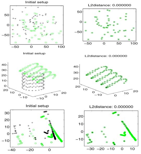
Results of rigid registration in noiseless case. ‘+’ and ‘o’ indicate the model and scene points respectively.

Next, to see how our method behaves in the presence of noise and outliers, we designed the following procedure to generate corrupted template point set from a model set. For a model set with n points, we control the degree of corruption by (1) discarding a subset of size (1 — ρ)n from the model point set, (2) applying a rigid transformation (R,t) to the template, (3) perturbing the points of the template with noise (of strength ∊), and (4) adding (τ — ρ)n spurious, uniformly distributed points to the template. Thus, after corruption, a template point set will have a total of τn points, of which only ρn correspond to points in the model set. Figure 2 shows some 2D results using our method. The model and scene points are represented by the ‘+’ and ‘o’ respectively in this figure. The arrangement is the same as before i.e., on the left is the model and superimposed (unregistered) template; on the right is the registered data after running our algorithm. We also display the L₂-distance between mixtures representing the two data sets after registration on top of each frame in the right column to indicate the precision of registration. A 3D example is also presented in Figure 3.

Figure 2.

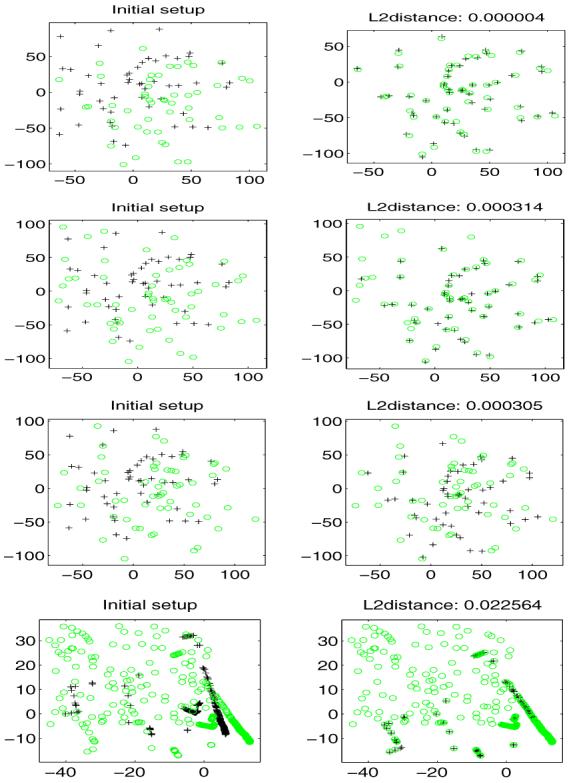
Tests on sensitivity to noise and outliers. From top to bottom in the left column: data with noise only; data with outliers (ρ =0.9, τ =1.1) and small noise; data with outliers (ρ = 0.9, τ = 1.1) and large noise; data corrupted by a large amount of outliers (ρ = 0.8, τ = 1.2). Right column depicts registration obtained using our algorithm.

Figure 3.

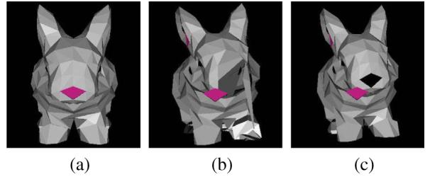
Robustness test on 3D bunny data. (a) bunny model with 427 points; (b) rotated model slightly corrupted by outliers (look near the left eye); (c) transformed model by recovered rotation.

Since ICP is known to be prone to outliers, we only compare our method with the more robust KC method in terms of the sensitivity of noise and outliers. The comparison is done via a set of 2D experiments. At each of several noise levels and outlier strengths, we generate five models and six corrupted templates from each model for a total of 30 pairs at each noise and outlier strength setting. For each pair, we use our algorithm and the KC method to estimate the known rigid transformation which was partially responsible for the corruption. Results show when the noise level is low, both KC and the presented method have strong resistance to outliers. However, we observe that when the noise level is high, our method exhibits stronger resistance to outliers than the KC method, as shown in Figure 4.

Figure 4.

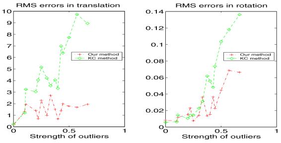
Robustness to outliers in the presence of large noise. Errors in estimated rigid transform vs. proportion of outliers ((τ — ρ)/(ρ)) for both our method and KC method.

4.2. Nonrigid Registration

In this part, we present our experiment results on nonrigid registration. Figure 5 demonstrates some results of our non-rigid point-set registration method applied to a set of 2D corpus callosum slices with feature points manually extracted by human experts. Our non-rigid method performs well on the presence of noise and outliers (Figure 5 right column). For purpose of comparison, we also tested the TPS-RPM program provided in [4] on this data set, and found that TPS-RPM can correctly register the pair without outliers (Figure 5 top left) but failed to match the corrupted pair (Figure 5 top right).

Figure 5.

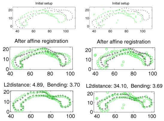
Nonrigid registration of corpus data. Top left: two manually segmented corpus callosum slices; Top right: same slices with one corrupted by noise and outliers; Middle: slices after affine registration; Bottom: slices after non-rigid registration.

5. Conclusions

Point set registration is a problem of pivotal importance that continues to attract considerable interest. In this work, we present a novel probabilistic modelling framework for point set registration which unifies some previous work in the field and exhibits better tolerance to outliers and is more computationally efficient than competing methods. By modeling each of the point set explicitly using a Gaussian mixture, we develop a robust and efficient registration based on a closed form expression for the L₂ distance between two Gaussian mixtures. Experiments on both synthetic and real data demonstrate the merits of our method. In our future work, we plan to study the applicability of mixture of distributions other than Gaussians and incorporate a diffeomorphic matching of distributions.

References

- [1].Fitzgibbon AW. Robust registration of 2D and 3D point sets. BMVC2001; 2001. [Google Scholar]
- [2].Granger S, Pennec X. Multi-scale EM-ICP: A fast and robust approach for surface registration. ECCV2002(4); 2002.pp. 418–432. [Google Scholar]
- [3].Huttenlocher DP, Klanderman GA, Rucklidge WA. Comparing images using the hausdorff distance. IEEE Trans. Pattern Anal. Mach. Intell. 1993;15(9):850–863. [Google Scholar]
- [4].Chui H, Rangarajan A. A new algorithm for non-rigid point matching. CVPR2000.pp. 2044–2051. [Google Scholar]
- [5].Chui H, Rangarajan A, Zhang J, Leonard CM. Un-supervised learning of an atlas from unlabeled point-sets. IEEE Trans. Pattern Anal. Mach. Intell. 2004;26(2):160–172. doi: 10.1109/TPAMI.2004.1262178. [DOI] [PubMed] [Google Scholar]
- [6].Guo H, Rangarajan A, Joshi S, Younes L. Non-rigid registration of shapes via diffeomorphic point matching. ISBI; 2004.pp. 924–927. [Google Scholar]
- [7].Belongie S, Malik J, Puzicha J. Shape matching and object recognition using shape contexts. IEEE Trans. Pattern Anal. Mach. Intell. 2002;24(4):509–522. [Google Scholar]
- [8].Tsin Y, Kanade T. A correlation-based approach to robust point set registration. ECCV2004(3).pp. 558–569. [Google Scholar]
- [9].Besl PJ, McKay ND. A method for registration of 3-D shapes. IEEE Trans. Patt. Anal. Machine Intell. 1992 February;14(2):239–256. [Google Scholar]
- [10].Chui H, Rangarajan A. A feature registration framework using mixture models. the IEEE Workshop on Mathematical Methods in Biomedical Image Analysis; 2000.pp. 190–197. [Google Scholar]
- [11].Scott D. Parametric statistical modeling by minimum integrated square Error. Technometrics. 2001;43(3):274–285. [Google Scholar]
- [12].Basu A, Harris IR, Hjort NL, Jones MC. Robust and efficient estimation by minimising a density power divergence. Biometrika. 1998;85(3):549–559. [Google Scholar]
- [13].Huber P. Robust Statistics. John Wiley & Sons; 1981. [Google Scholar]
- [14].Goldberger J, Gordon S, Greenspan H. An efficient image similarity measure based on approximations of KL-divergence between two gaussian mixtures. ICCV03; 2003; France: Nice; pp. 487–493. [Google Scholar]
- [15].Singh MK, Arora H, Ahuja N. Robust registration and tracking using kernel density correlation. The Second IEEE Workshop on Image and Video Registration; 2004.pp. 174–182. [Google Scholar]
- [16].Greengard L, Strain J. The fast Gauss transform. SIAM Journal of Scientific Computing. 1991;12(1):79–94. [Google Scholar]