Metachronal wave formation in a model of pulmonary cilia

Abstract

A three-dimensional simulation of the formation of metachronal waves in rows of pulmonary cilia is presented. The cilia move in a two-layer fluid model. The fluid layer adjacent to the cilia bases is purely viscous while the tips of the cilia move through a viscoelastic fluid. An overlapping fixed-moving grid formulation is employed to capture the effect of the cilia on the surrounding fluid. In contrast with immersed boundary methods, this technique allows a natural enforcement of boundary conditions without the need for smoothing of singular force distributions. The fluid domains are discretized using a finite volume method. The 9 + 2 internal microtubule structure of an individual cilium is modeled using large-deflection, curved, finite-element beams. The microtubule skeleton is cross-linked to itself and to the cilium membrane through spring elements which model nexin links. The cilium membrane itself is considered to be elastic and subject to fluid stresses computed from the moving grid formulation as well as internal forces transmitted from the microtubule skeleton. A cilium is set into motion by the action of dynein molecules exerting forces between adjacent microtubules. Realistic models of the forces exerted by dynein molecules are extracted from measurements of observed cilia shapes.

1. Introduction

One of the main protective mechanisms of the lung is a fluid layer coating the interior epithelial surfaces of the bronchi and bronchioles. This is known as the airway surface liquid (ASL) and it varies in thickness from 5 to 100 μm [36]. The ASL exhibits a two-layer structure. Adjacent to the epithelium one finds a region of low-viscosity fluid known as the periciliary layer (PCL) which is widely thought to exhibit Newtonian behavior [21]. The PCL is typically 7 μm thick. Cilia sprout from the epithelial layer. It has been observed that cilia lengths are comparable to the PCL thickness under healthy conditions [36]. The cilia beat in a coordinated fashion within the PCL layer [15]. The region between the PCL and the airway is occupied by a more viscous mucus layer. Under normal healthy conditions the mucus is a viscoelastic fluid with a typical thickness of 30 μm in humans. The tips of the cilia have been observed to penetrate the bottom portion of the mucus layer during their beat cycle [36]. Ciliar motion leads to entrainment of the ASL, propelling it towards the trachea and then out of the body or into the gastro-intestinal tract. This process is known as mucociliary transport. It is hypothesized that the PCL serves both as a lubricant to allow motion of the viscous mucus layer and as a lower-viscosity medium more favorable to the motion of cilia. Foreign objects present in the bronchi and bronchioles (e.g. inhaled particulates, bacteria spores) are trapped in the viscous mucus layer. Mucociliary transport then ensures elimination of these foreign objects from the lung. The proper functioning of this process is fundamental to maintaining a healthy state. A major disease associated with the breakdown of mucociliary transport is cystic fibrosis [34]. Specific genetic defects associated with cystic fibrosis lead to reduced mucociliary transport leaving the lung subject to chronic infections from, e.g. bacteria spores that are not eliminated from the bronchioles. Other mechanisms can eliminate the foreign objects (cough, airway constrictions, see [14]), but a fundamental observation is that the healthy state is characterized by a functioning mucociliary transport while other mechanisms such as cough are invoked as a response to a diseased state.

Though the overall picture of mucociliary transport is qualitatively understood, the details are unclear. The velocity distribution within the layers has long been open to conjecture [21]. The role of ciliar beating in effective entrainment has not yet been elucidated. Models of reduced dimensionality have been presented [15,4] in which various other simplifications of the physical model are also introduced, in particular the fluid force acting on a cilium is typically estimated from a generalized Stokes law. The exact mechanism by which cilia coordinate their motion in order to produce overall motion has also been open to speculation. Hydrodynamic interactions have long been proposed as a principal mechanism [32], but there also remains the possibility of elastic coupling through the endothelium layer or synchronization through biochemical signaling.

The present research seeks to provide the computational tools for testing hypotheses about the mechanisms of mucociliary transport. Examples of the questions that can be addressed by the present computational framework are:

1. Is mucociliary transport produced by cilia motion alone? (Alternative or additional mechanisms include Maragnoni transport, [6].)

2. How is cilia coordination achieved?

3. How do cilia respond when the PCL thickness is reduced?

4. At what mucus viscosity is cilia penetration into the mucus impeded?

Directly answering these physiological or biomedical questions is not addressed here, but will be the subject of subsequent papers. The focus is rather on the physical and mathematical model for entrainment of the ASL by ciliar beating, an attempt being made to realistically and quantitatively capture all relevant details. Essentially, the model is a fluid-structure interaction (FSI) problem with the following distinguishing features:

1. The elastic structure is of biological origin.

2. There are two types of fluids: Newtonian and viscoelastic.

3. The elastic structure is composed of very many individual cilia that undergo large deformations.

The remainder of the paper is organized as follows. Section 2 describes the biological system to be modeled. Section 3 presents the physical and numerical models for the component parts of the system. Section 4 presents typical results focusing on answering the question of how ciliar coordination is achieved through hydrodynamic interactions. Conclusions and further work are presented in Section 5.

2. Cilium morphology

A cilium is a thin filament with a 30:1 ratio between length and diameter. Electron micrographs such as Fig. 1A reveal the remarkable internal structure of a cilium. A sharper image of the transverse structure is shown in Fig. 1B. The cilium exhibits a load bearing structure composed of microtubules (Fig. 1B(a) and (b)) placed on a circle towards the periphery of the cilium cross-section. Microtubules are filamentary structures formed by repetition of a tubulin dimer macromolecule. The “A” microtubule (Fig. 1B(a)) has a circular cross-section and the “B” microtubule (Fig. 1B(b)) a “C” cross-section. In addition to the peripheral microtubules the cilium contains a central pair (Fig. 1B(d)) that induces a preferred bending direction. The central microtubules are linked to a loosely defined central sheath (Fig. 1B(f)) that is in it turn linked to the peripheral “A” microtubules through central spokes (Fig. 1B(c)). The peripheral microtubules are linked to the surrounding cilium membrane. Peripheral microtubules are linked to one another through passive nexin links and active dynein links. The dynein molecular motor [1] is a complex molecule that in the presence of ATP (adenosine triphosphate) carries out a stepping motion in which alternating globular heads of the dynein molecule successively attach and detach to the tubulin dimer pairs of a microtubule, thereby exerting a small force between microtubules. The dark regions (Fig. 1B(e)) adjacent to a microtubule are arms of the dynein molecule. The cumulative effect of all ∼4000 active dynein molecules within a cilium leads to an overall bending motion that drives the surrounding fluid. The overall load-bearing structure of the cilium is referred to as the cilium axoneme. One can describe a cilium as a membrane enclosing an interior fluid region containing the axoneme.

Fig. 1.

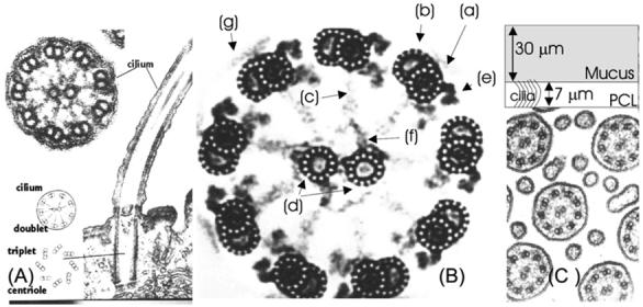
(A) Electron micrograph of cilium showing longitudinal and transverse sections. (B) Detailed electron micrograph of a transverse section through a cilium showing the 9 + 2 microtubule structure and the internal structure of microtubules. (C) Micrograph: relative spacing between cilia. Sketch: two-layer structure of ASL. (Micrographs are copyright Gwen C. Childs, www.cytochemistry.net/Cell-biology/cilia.htm.)

The cilia move mostly within the PCL layer, their tips at times penetrating into the more viscous mucus layer. Increase of mucin concentrations in the mucus can lead to ineffective cilia motion or stoppage. Typical dimensions of a cilium are presented in Table 1.

Table 1.

Typical cilium dimensions (in nanometers)

Cilium diameter, D	225
Microtubule exterior diameter, D1	25
Microtubule interior diameter, D2	14
Cilium length, L	7000
Microtubule centers diameter, D0	170

Devising a quantitative model of mucociliary clearance is challenging due to the disparity in scales between the molecular motors driving a cilium and the length scale representative of ASL transport, typically a region covering a few hundred cells. The representative length scale for the driving force is the distance between adjacent microtubules l ∼ 60 nm, while that for the ASL flow is L ∼ 400 μm a disparity of almost 4 orders of magnitude.

3. Mechanical models of cilium axoneme components

A three-dimensional model of the internal mechanical behavior of a cilium is introduced based upon approximating microtubules as thin-walled beams and the connecting dynein and nexin elements as forces and springs, respectively. Previous work on cilium axoneme models includes that of Blake [4] and Gueron et al. [15] in which the cilium has no internal structure and the two-dimensional model of Dillon et al. [8] in which microtubules are modeled by a pair of inextensible filaments with no flexural resistance linked by diagonal springs to confer overall flexural rigidity for the axoneme. Dillon et al. also use spring elements to model nexin and radial (spoke) links. In the following, experimental measurements of microtubule flexural behavior are presented to argue that the intrinsic flexural rigidity is important in the overall mechanical behavior of a microtubule.

3.1. Physical properties

A brief summary of known mechanical properties of the biological components relevant to mucociliary flow is presented. Based on these properties specific mechanical models are chosen for each component. The mathematical details of the models are presented in Sections 3.2 and 3.3. It should be noted that the data presented here is affected by the difficulty in obtaining mechanical properties for microscopic biological materials. This constitutes one of the chief uncertainties of the overall model. One of the objectives of the present research is to establish bounds on these physical values consistent with observed ciliar motion.

3.1.1. Microtubules

Experimental work of Gittes et al. [12] has shown that the flexural rigidity of single, taxol-stabilized microtubules is significant, EI = 2.19 ± 0.18 × 10^-23 N m². The flexural rigidity was determined by analyzing thermal fluctuations in shape. Direct bending of a microtubule using optical tweezers has been carried out by Felgner et al. [10]. They measured a flexural rigidity EI = 1.0 ± 0.3 × 10^-24 N m² for taxol-stabilized microtubules and EI = 3.7 ± 0.8 × 10^-24 N m² for pure microtubules. Van Mameren obtains a value of EI = 4.2 ± 0.4 × 10^-24 N m² again using optical tweezers. There is a significant variance in these results. We can however estimate 10^-24 N m² ≲ EI ≲ 10^-23 N m² to give an order-of-magnitude estimate of flexural rigidity. The typical force exerted by a dynein molecule on a microtubule has been measured by Shingyoji et al. [30] as F ≈ 6 × 10^-12 N. A force of this magnitude applied to a cantilevered beam with a flexural rigidity of EI = 2.19 ± 0.18 × 10^-23 N m² at a distance of l = 3 × 10^-6 m from the support (roughly the midpoint of a cilium) leads to a deflection of δ = Fl³/3EI = 2.5 × 10^-6 m which though large, does show that microtubule rigidity is high enough to store as deformation energy the work done by a single dynein molecule. It is therefore of interest to construct a mechanical model with realistic models of microtubule flexural rigidity. Recent studies [27] of grafted microtubules suggest anisotropic behavior. Though this is to be expected due to microtubule construction from a periodic array of tubulin dimers, the anisotropic elastic moduli are uncertainly measured at present. Hence, isotropic behavior will be used in the computations here.

3.1.2. Nexin links, microtubule-membrane links, and radial spokes

There are few available measurements of the mechanical properties of the nexin links and radial spokes present in the axoneme. Experimental observations [25] suggest that these are elastic strings. Analysis of measured forces when an axoneme is subject to longitudinal shearing [23] suggest a spring constant of k = 2 pN/nm for the nexin links. Similar protein complexes, but of much shorter length, link the microtubules to the membrane and these are modeled by stiffer springs with k = 200 pN/nm in the absence of more detailed experimental observation. This links a microtubule almost rigidly to the immediate portion of cilium membrane adjacent to it. The spokes are modeled as springs with k = 10 pN/nm [23].

3.1.3. Dynein motors

The force exerted by a single dynein molecule upon a microtubule has been the subject of extensive experimental effort. A peak value of F = 6 pN has been observed experimentally [33]. Though the force exerted by one dynein molecule is relatively well known, the exact mechanism by which the dynein molecules in an axoneme act cooperatively to produce an overall motion is still not clear. Various ad hoc mechanisms have been proposed. These include the geometric clutch model of Lindeman [19] and the curvature controlled model of Dillon et al. [8]. A separate research effort [24] is underway to determine these forces as a function of microtubule positions from a first principle computation using a random walker model of dynein molecules on the microtubule structures. Proof-of-concept computations for the fluid-structure interaction problem considered here are carried out with an assumed, analytical form presented below.

3.1.4. Cilium membrane and central sheath

The cilium membrane is a bilipid layer as found in a wide variety of cells. The mechanical properties of such layers can be found by atomic force microscopy (e.g. [38]) or dilation of membrane vesicles and the surface extensional stiffness is in the range γ = 10^-2 - 10^-1 pN/nm [9]. A value of γ = 0.5 pN/nm is used here. The exact structure of the central sheath is unknown at present. The protein composition seems to be similar to that of the nexin and radial spokes so a value of γ = 1 pN/nm is used here.

3.1.5. PCL

The periciliary liquid is hypothesized to be a saline solution that exhibits Newtonian behavior. A dynamic viscosity value of μ = 10^-3 Pa s [31] is adopted.

3.1.6. Mucus

Mucus is an extremely complicated biofluid containing a number of mucin macromolecules that impart viscoelastic behavior [28,17]. A full viscoelastic characterization is not yet available. An active program that seeks to fully describe the rheology of mucus is underway at the University of North Carolina as part of the Virtual Lung project. A good starting point is to assume an upper convected Maxwell model [3]. For mucus with a mass concentration of 2% mucins the principal relaxation time has been found to be λ = 3 s. The mucus viscosity is μ_s = ρ_sν_s = 10^-1 Pa s (ρ_s = 1010 kg/m³). The additional viscoelastic stress is generated proportional to strain fields within the mucus with a constant of proportionality μ_p = 10^-3 Pa s.

3.2. Cilium axoneme mechanical model

3.2.1. Geometric description

The cilium shape is described by a set of curves passing through the centers of each microtubule. For cilia with a 9 + 2 internal structure 11 curves are required

$${\overrightarrow{R}}_i(s,t)=x_i(s,t)\widehat{i}+y_i(s,t)\widehat{j}+z_i(s,t)\widehat{k},i=1,\dots ,11$$ (1)

with s representing arc length measured from cilium base and t time. At any point along a microtubule centerline the Frenet triad is used to define a local coordinate system. The tangent, normal and binormal vectors are given by

$$\stackrel{‒}{T}=\frac{\partial \overrightarrow{R}}{\partial s},\overrightarrow{N}=\frac{1}{\kappa }\frac{\partial \overrightarrow{T}}{\partial s},\overrightarrow{B}=\frac{1}{\tau }\left(\frac{\partial \overrightarrow{N}}{\partial s}+\kappa \overrightarrow{T}\right)$$ (2)

with κ the curvature and τ the torsion of the centerline curve. The shape of the cross-section of a microtubule is given as a polar curve

$$r=r\left(\theta \right).$$ (3)

3.2.2. Elastic springs model for nexin, radial spokes

An elastic spring element is described in a local coordinate system with the s-axis along the spring length. The element has two nodes i and j with nodal displacements $U^e={\left[u_i{u}_j\right]}^{\mathrm{T}}$ and nodal forces oriented along the s-axis $F^e={\left[f_i{f}_j\right]}_j^{\mathrm{T}}$. The rigidity matrix K^e of the element specifies the linear dependence of forces upon displacements, F = KU and is given by

$$K^e=\left[\begin{array}{cc}\hfill k\hfill & \hfill -k\hfill \\ \hfill -k\hfill & \hfill k\hfill \end{array}\right]$$ (4)

with k the element’s spring constant.

3.2.3. Beam model for microtubules

Each microtubule or microtubule doublet is modeled as a thin-walled beam (Fig. 2). A total Lagrangian Timoshenko beam element is used [2,16]. For details on derivation see [11,7]. The curved beam element has 6 degrees of freedom per node and two nodes per element. The 6 displacements defined at each node are 3 linear displacements (u, v, w) along the $(\overrightarrow{T},\overrightarrow{N},\overrightarrow{B})$ directions and 3 rotations (α, β, γ) around the $(\overrightarrow{T},\overrightarrow{N},\overrightarrow{B})$ axes. The angular displacement α specifies the section twist, while β, γ give the section’s rotation. The displacements produce forces (V_T, V_N, V_B) and moments (M_T, M_N, M_B) within the cross-section. Let U be the general displacement vector and F the general force vector at a node i

$$U_i={\left[u_i{v}_i{w}_i{\alpha }_i{\beta }_i{\gamma }_i\right]}^{\mathrm{T}},$$ (5)

$$F_i={\left[V_{T,i}{V}_{N,i}{V}_{B,i}{M}_{T,i}{M}_{N,i}{M}_{B,i}\right]}^{\mathrm{T}}.$$ (6)

The element displacement vector, force vector are

$$U^e=\left[\begin{array}{c}\hfill U_i\hfill \\ \hfill U_j\hfill \end{array}\right],F^e=\left[\begin{array}{c}\hfill F_i\hfill \\ \hfill F_j\hfill \end{array}\right].$$ (7)

The element force vector is a function of the displacements F^e = F^e(U^e). Due to the large deflections typical of ciliar motion the relationship between forces and displacements is nonlinear. The rigidity matrix is given by the Jacobian

$$K_0^e=\frac{\partial F^e}{\partial U^e}\left(U_0^e\right)$$ (8)

and can be written as the sum of a material stiffness matrix and a geometric stiffness matrix

$$K_0^e=K_m+K_G.$$ (9)

A ${\mathcal{C}}^0$ interpolation is used to describe displacements within the element. Shear locking is eliminated through the simple residual bending flexibility correction [20]. For completeness, the detailed form of the stiffness matrix for plane beams is presented in Appendix A as taken from [11].

Fig. 2.

(a) Curved beam element. At nodes i, j a local coordinate system is defined based on the Frenet triad. Six displacements, three forces and three moments are defined at each node. (b) Transverse section of cilium model. Microtubules are modeled as thin-walled beams. They are connected by elastic springs modeling nexin and dynein links. The entire structure is enclosed in an elastic outer membrane. An inner membrane surrounds the two central microtubules. It is linked by elastic springs to each microtubule; the springs model the radial spokes of real cilia.

3.3. Airway surface liquid model

3.3.1. Periciliary layer

The layer of approximate thickness l = 7 μm in the immediate vicinity of the endothelium layer is considered to be a Newtonian fluid. Due to the small scales involved, the unsteady Stokes equations are an appropriate model

$$\begin{array}{c}\hfill \nabla \cdot \overrightarrow{v}=0,\text{in}\Omega ,\hfill \\ \hfill {\overrightarrow{v}}_t+{\nabla }_p=\nu {\nabla }^2\overrightarrow{v},\text{in}\Omega ,\hfill \\ \hfill \overrightarrow{N}\cdot \overrightarrow{v}=\overrightarrow{N}\cdot {\overrightarrow{V}}_{\text{cilium}},\overrightarrow{T}\cdot \overrightarrow{v}=0,\text{on}\partial \Omega ,\hfill \end{array}$$ (10)

with ${\overrightarrow{V}}_{\text{cilium}}$ the local cilium velocity. The time derivative of the velocity ${\overrightarrow{v}}_t$ is kept since it is not evident a priori that the diffusive transport of momentum in the Stokes fluid is fast enough to dissipate the local effect of ciliar forcing. The above equations are solved on two overlapping domains. An overall rectangular domain contains the entire PCL. On this boundary far-field boundary conditions (e.g. periodicity) are applied. Around each cilium individual, curvilinear, time-deforming grids are constructed. This technique allows the surface boundary conditions on the cilium membrane to be easily applied. In order to maintain overall efficiency of the model the grids around a cilium are constructed as a deformation of a cylindrical grid, maintaining orthogonal coordinates in each cross-section. This allows Fourier transforms to be applied and a fast Poisson solver to be used in solving the finite-volume discretization of the Stokes equations.

Cilium curvilinear grid

An overall median line is established for each cilium given by

$${\overrightarrow{R}}_c(s,t)=X(s,t)\widehat{i}+Y(s,t)\widehat{j}+Z(s,t)\widehat{k}$$

in the Cartesian unit basis vectors $(\widehat{i},\widehat{j},\widehat{k})$. The grid mapping (x, y, z, t) ↔ (s, θ, r, t) defined by

$$\overrightarrow{R}(s,\theta ,r,t)=X(s,t)\widehat{i}+Y(s,t)\widehat{j}+Z(s,t)\widehat{k}+r[\cos \theta \overrightarrow{N}(s,t)+\sin \theta \overrightarrow{B}(s,t)]$$ (11)

is introduced. The curvilinear basis vectors are

$$\begin{array}{c}\hfill {\overrightarrow{u}}_s=\frac{\partial \overrightarrow{R}}{\partial s}=(1-\kappa r\cos \theta -\tau r\sin \theta )\overrightarrow{T}+\tau r\cos \theta \overrightarrow{B},\hfill \\ \hfill {\overrightarrow{u}}_{\theta }=\frac{\partial \overrightarrow{R}}{\partial \theta }=-r\sin \theta \overrightarrow{N}+r\cos \theta \overrightarrow{B},{\overrightarrow{u}}_r=\frac{\partial \overrightarrow{R}}{\partial r}=\cos \theta \overrightarrow{N}+\sin \theta \overrightarrow{B}.\hfill \end{array}$$

Note that if the torsion is null τ = 0 we have

$${\overrightarrow{u}}_s=\frac{\partial \overrightarrow{R}}{\partial s}=(1-\kappa r\cos \theta )\overrightarrow{T}$$

and the $({\overrightarrow{u}}_s,{\overrightarrow{u}}_{\theta },{\overrightarrow{u}}_r)$ is orthogonal. This would indeed hold for in-plane bending of a cilium for which there is experimental evidence [15] (in the absence of diseased conditions associated with the abnormal motions known as ciliar dyskinesia). Under these conditions the curvilinear nabla operator is

$$\nabla =\frac{{\overrightarrow{u}}_s}{1-\kappa r\cos \theta }\frac{\partial }{\partial s}+\frac{{\overrightarrow{u}}_{\theta }}{r}\frac{\partial }{\partial \theta }+{\overrightarrow{u}}_r\frac{\partial }{\partial r}$$

and the curvilinear Laplace operator is

$${\nabla }^2\varphi =\frac{1}{{(1-\kappa r\cos \theta )}^2}\frac{{\partial }^2\varphi }{\partial s^2}+\frac{1}{2}\frac{\partial \varphi }{\partial s}\frac{\partial }{\partial s}\left[\frac{1}{{(1-\kappa r\cos \theta )}^2}\right]+\frac{1}{r^2}\frac{{\partial }^2\varphi }{\partial {\theta }^2}+\frac{1}{r}\frac{\partial \varphi }{\partial \theta }\frac{\partial }{\partial \theta }\ln (1-\kappa r\cos \theta )+\frac{{\partial }^2\varphi }{\partial r^2}+\frac{\partial \varphi }{\partial r}\frac{\partial }{\partial r}\ln \left[r(1-\kappa r\cos \theta )\right].$$

This formulation is used in the flow equations (10).

3.3.2. Mucus layer

The mucus layer is modeled through an upper convected Maxwell model [3] described by

$$\nabla \cdot \overrightarrow{v}=0,\text{in}\Omega ,$$

$${\overrightarrow{v}}_t+(\overrightarrow{v}\cdot \nabla )\overrightarrow{v}+{\nabla }_p={\nu }_s{\nabla }^2\overrightarrow{v}+\nabla \cdot \tau ,\text{in}\Omega ,$$

$${\tau }_t+(\overrightarrow{v}\cdot \nabla )\tau -\nabla {\overrightarrow{v}}^{\mathrm{T}}\tau -\tau \nabla \overrightarrow{v}=2{\mu }_{\mathrm{p}}\mathbf{D}-\tau ∕\lambda ,\text{in}\Omega ,$$

$$2\mathbf{D}=\nabla \overrightarrow{v}+\nabla {\overrightarrow{v}}^{\mathrm{T}},$$

$$\overrightarrow{N}\cdot \overrightarrow{v}=\overrightarrow{N}\cdot {\overrightarrow{V}}_{\text{cilium}},\overrightarrow{T}\cdot \overrightarrow{v}=0,\text{on}\partial {\Omega }_{\text{cilium}},$$

with material properties presented in Section 3.1.6. Here τ is the additional viscoelastic stress tensor which is symmetric, and $\nabla \overrightarrow{v}$ is velocity gradient tensor.

3.4. Dynein forces

The final component of the mechanical model of a cilium is the force exerted by the dynein molecular motors. For the proof-of-concept computations carried out here the dynein forces are determined by least-squares fitting to observed single-cilium beat patterns. Such patterns are being actively collected and cataloged at the University of North Carolina [29]. The force between the m A-microtubule and the adjacent (m + 1) B-microtubule is assumed to depend on the longitudinal position s and time t through the following analytical form:

$$F_{\text{dynein}}^{\left(m\right)}(s,t)=p^{\left(m\right)}\left(s\right)\cos (k^{\left(m\right)}s-\omega t+{\varphi }^{\left(m\right)}).$$ (12)

Here p^(m)(s) is a cubic spline interpolant defined at the same nodal positions as used for the microtubule beam, k^(m) is the dominant cilium beat-shape wavenumber and ω is the measured cilium beat frequency. The phase ϕ^(m) is set to zero for the single-cilium analysis but will be allowed to vary when computing cilia arrays. The spline coefficients a^(m) in p^(m)(s) and k^(m) are unknown parameters in the microtubule interaction force. They are determined by least squares fitting of the cilium beat shape obtained from solving (17) to observed beat shapes. Let {t¹ , ... , tⁿ} be the times at which a cilium beat shape is observed (e.g. Fig. 4). The function

$$S(a^{\left(m\right)},k^{\left(m\right)})=\sum _{l=1}^n{[\overrightarrow{ℱ}\left(X\left(t^l\right)\right)-\overrightarrow{x}\left(t^l\right)]}^2$$

describes the error between the observed mean fiber beat shape $\overrightarrow{x}\left(t^n\right)$ and that deduced from the microtubule nodal positions X(tⁿ) through the function $\overrightarrow{ℱ}$ (e.g. average over nodal coordinates). The parameters (a^(m), k^(m)) are determined from

$$\frac{\partial S}{\partial a_j^m}=0,\frac{\partial S}{\partial k^m}=0,m=1,\dots ,11;j=1,\dots ,N+1$$

with N the number of beam elements used to discretize a microtubule m.

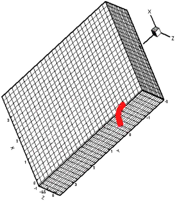
Fig. 4.

The sequence of cilium centerline shapes defining a beat-pattern body-fitted grid. Red shows the cilium in the power stroke and blue in the recovery stroke.

Given that the internal dynein forces are determined from experimental fitting, the present model does not predict an individual cilium beat shape from first principles. The main interest is to investigate multiple cilia coordination by allowing ϕ^(m) to assume different values at adjacent cilia. This is presented below.

4. Numerical algorithms

4.1. The Stokes equations

Eq. (10) are discretized on the curvilinear grid around each cilium and also on the overall Cartesian grid covering the PCL. A finite-volume spatial discretization technique leads to an ODE system that is to be integrated in time. A projection method [5] using a gauge transformation

$$\overrightarrow{v}=\overrightarrow{a}+\nabla \varphi$$ (13)

decouples the diffusive momentum transport

$$\{\begin{array}{cc}{\overrightarrow{a}}_t=\nu {\nabla }^2\overrightarrow{a},\hfill & \text{in}\Omega ,\hfill \\ \overrightarrow{N}\cdot \overrightarrow{a}=\overrightarrow{N}\cdot {\overrightarrow{V}}_{\text{cilium}},\hfill & \overrightarrow{T}\cdot \overrightarrow{a}=-\frac{\partial \varphi }{\partial T},\text{on}\partial {\Omega }_{\text{cilium}},\hfill \end{array}\phantom{\}}$$

from the pressure effects encoded in

$$\{\begin{array}{cc}{\nabla }^2\varphi =-\nabla \cdot \overrightarrow{a},\hfill & \text{in}\Omega ,\hfill \\ \frac{\partial \varphi }{\partial \overrightarrow{N}}=0,\hfill & \text{on}\partial {\Omega }_{\text{cilium}}.\hfill \end{array}\phantom{\}}$$

The diffusion equation is solved using a Crank-Nicolson method and the pressure correction is computed by an FFT-based fast Poisson solver. The fast Poisson solver is expressed in Cartesian coordinates for the background grid and in the curvilinear coordinates (11) for the cilium grid. The Crank-Nicolson step for the Stokes equations can be obtained from that for the viscoelastic equation (15) by setting τ = 0 and neglecting the convective term $(\overrightarrow{v}\cdot \nabla )\overrightarrow{v}$. The approach is similar to that in [35] and allows for efficient simulation of the incompressible flow.

4.2. The viscoelastic equations

The Maxwell model viscoelastic equations are solved using a similar approach. After introducing the gauge transform (13) we obtain

$$\{\begin{array}{cc}{\overrightarrow{a}}_t+(\overrightarrow{v}\cdot \nabla )\overrightarrow{v}={\nu }_s{\nabla }^2\overrightarrow{a}+\nabla \cdot \tau ,\hfill & \text{in}\Omega ,\hfill \\ \overrightarrow{N}\cdot \overrightarrow{a}=\overrightarrow{N}\cdot {\overrightarrow{V}}_{\text{cilium}},\hfill & \overrightarrow{T}\cdot \overrightarrow{a}=-\frac{\partial \varphi }{\partial T},\text{on}\partial {\Omega }_{\text{cilium}},\hfill \end{array}\phantom{\}}$$

where the convective term $(\overrightarrow{v}\cdot \nabla )\overrightarrow{v}$ has been maintained for the mucus layer. The additional viscoelastic stress τ arises as a source term in the above equation. Its evolution is computed from the equation

$${\tau }_t+(\overrightarrow{v}\cdot \nabla )\tau -\nabla {\overrightarrow{v}}^{\mathrm{T}}\tau -\tau \nabla \overrightarrow{v}=2{\mu }_{\mathrm{p}}\mathbf{D}-\tau ∕\lambda ,\text{in}\Omega ,$$

which is typically dominated by the convective terms on the lhs. It is advanced in time using the wave propagation approach of LeVeque [18] to obtain τⁿ⁺¹, the viscoelastic stress at the next time level n + 1 starting from quantities defined at time level n.

Two types of boundaries arise: fluid-fluid interfaces and fluid-solid interfaces where a cilium penetrates the mucus layer. At both types of interface we must have overall continuity of the stress. At a fluid-fluid interface this can be written as

$$[\sigma +pI+\tau ]=0$$ (14)

σ is the fluid viscous stress tensor, p is the pressure, I the identity matrix and [ ] denotes the difference between the quantities enclosed in brackets between the two interface sides. Capillary and other surface effects are neglected.

Determining appropriate boundary conditions for the viscoelastic τ stress is a research topic in itself. In (14) there seem to be more unknowns than conditions such that we could freely choose τ. This is due to the fact that the additional stress in the viscoelastic fluid arises from the microscopic, configurational state of the polymers conferring viscoelastic behavior. This microscopic information is not available at the continuum level considered here. Formalisms on which to provide a rational closure are under investigation [37,13,26]. These depend on the specific polymeric fluid involved, and as such are difficult to apply to mucus the detailed composition of which is uncertain. An ad hoc approach is adopted here. The main modeling question to be addressed is to determine what part of the stress from the Newtonian fluid leads a viscoelastic stress τ. In the absence of additional experimental information the following hypothesis is used:

$$\frac{1}{2}{\sigma }_1\cdot \mathbf{t}={\sigma }_2\cdot \mathbf{t},\frac{1}{2}{\sigma }_1\cdot \mathbf{t}=\tau \cdot \mathbf{t},\tau \cdot \mathbf{n}=0.$$

This amounts to stating that half of the tangential stress from within the Newtonian fluid (subscript 1) is transferred to the tangential viscous stress within the viscoelastic fluid (subscript 2) and half to the viscoelastic extra stress. There is no transfer of normal stress to the viscoelastic stress component. A solid-viscoelastic boundary that arises in this computation occurs when the tip of a cilium penetrates into the mucus layer. A hypothesis similar to the above is made in which half of the normal stress acting on the elastic membrane is given by pressure and normal viscous stress (pI + σ) · n and half by viscoelastic stress τ · n. The tangential viscoelastic stress is assumed zero at solid-fluid boundaries τ · t = 0.

The gauge variable equation is advanced in time using a Crank-Nicolson scheme. The full equation set is presented to show the extrapolation used for convective effects and how boundary conditions are imposed

$$\{\begin{array}{c}\frac{{\overrightarrow{a}}^{n+1}-{\overrightarrow{a}}^n}{\Delta t}+({\overrightarrow{v}}^{n+1∕2}\cdot \nabla ){\overrightarrow{v}}^{n+1∕2}=\frac{{\nu }_s}{2}{\nabla }^2({\overrightarrow{a}}^n+{\overrightarrow{a}}^{n+1})+\nabla \cdot {\tau }^{n+1∕2},\hfill \\ ({\overrightarrow{v}}^{n+1∕2}\cdot \nabla ){\overrightarrow{v}}^{n+1∕2}=\frac{3}{2}({\overrightarrow{v}}^n\cdot \nabla ){\overrightarrow{v}}^n-\frac{1}{2}({\overrightarrow{v}}^{n-1}\cdot \nabla ){\overrightarrow{v}}^{n-1},\hfill \\ {\overrightarrow{N}}^{n+1}\cdot {\overrightarrow{a}}^{n+1}={\overrightarrow{N}}^{n+1}\cdot {\overrightarrow{V}}_{\text{cilium}}^{n+1},{\overrightarrow{T}}^{n+1}\cdot \overrightarrow{a}=-\left(2\frac{\partial {\varphi }^n}{\partial T}-\frac{\partial {\varphi }^{n-1}}{\partial T}\right).\hfill \end{array}\phantom{\}}$$ (15)

Finally the pressure correction is computed using an FFT-based fast Poisson solver

$$\{\begin{array}{c}{\nabla }^2{\varphi }^{n+1}=-\nabla \cdot {\overrightarrow{a}}^{n+1},\text{in}\Omega ,\hfill \\ \frac{\partial \varphi }{\partial N}=0,\text{on}\partial {\Omega }_{\text{cilium}}.\hfill \end{array}\phantom{\}}$$

4.3. Overlayed grid communication

The computational simulation in the immediate vicinity of each cilium is carried out on a local, body fitted grid that deforms in response to the deformation of the cilium mean fiber as given by (11). Each cilium grid interacts with an overall background Cartesian grid. The background grid transmits cilium-cilium interactions and far-field boundary conditions. This approach presents several advantages: (1) boundary conditions can be imposed on the cilium membrane directly; (2) the individual cilia computations are decoupled and hence easily parallelized over a time step. This second aspect is crucial in attaining the final goal of computation over a realistic number of cilia.

The question arises of ensuring grid communication between the local curvilinear grids and the background Cartesian grids. The role of the Cartesian background grid is to efficiently transfer far-field boundary conditions while that of the cilium grid is to transmit the forcing effect of the cilium. At each time step the following procedure is adopted:

1. The velocity and pressure fields from the background Cartesian grid $({\overrightarrow{v}}^n,p^n)$ are used to form boundary values for the individual cilia grids using bilinear interpolation. Each grid point on the cilium curvilinear grid is enclosed in a Cartesian background grid cell. Let {Q_ijk} be the eight nodal values from the background grid. The interpolation valid over this background cell is

   $$\begin{array}{c}\hfill q(\xi ,\eta ,\zeta )=\sum _{l=1}^8{Q}_{ijk}{N}_l(\xi ,\eta ,\zeta ),\hfill \\ \hfill N_l(\xi ,\eta ,\zeta )=\frac{1}{8}(1\pm \xi )(1\pm \eta )(1\pm \zeta ).\hfill \end{array}$$ (16)

2. The fluid equations in each cilium, body fitted grid are solved to obtain $({\overrightarrow{v}}_c^n,p_c^n)$.

3. The cilium values are used to update values of the background nodes that fall within cilia body-fitted grids, leading to the values $({\overrightarrow{v}}^{\ast },p^{\ast })$. For background nodes not in any of the cilium grids we have $({\overrightarrow{v}}^{\ast },p^{\ast })=({\overrightarrow{v}}^n,p^n)$. The background grid is then advanced from these initial values. Given the elliptic nature of the pressure equation within the Stokes system, this procedure effectively introduces a surface layer potential at interfaces between cilia grids and background grids, in theory leading to a fall to first-order accuracy of the base second-order procedure used for advancing the Stokes equation solution. However given the extremely elongated shape of cilia, which transfers to the body fitted grids, there is a minimal drop in order-of-accuracy, essentially because the induced surface layer potentials correspond to jumps in the pressure over a small number of nodes in comparison to the overall number of nodes in the computation [22].

4.4. Fluid-structure interaction

Assembly of the cilium axoneme finite element model leads to an equation

$$M\ddot{X}+KX=F_{\text{fluid}}\left(t\right)+F_{\text{dynein}}\left(t\right),$$ (17)

where X is the vector of all microtubule beam element displacements and all nexin spring displacements. A lumped-mass model is employed to determine the mass matrix M. The force exerted by the dynein molecules is assumed to be specified a priori, e.g. as presented in Section 3.4. The main question for the FSI problem is how to compute F_fluid. One simplifying consideration in the mucociliary transport problem is that the volume of each cilium does not change so there is no need to solve a strongly coupled problem between fluid stresses and surface elastic stresses on the cilium membrane. This allows the computation of the fluid forces from a given kinematic state of the cilia.

A splitting procedure results in which to advance from time step tⁿ to time step tⁿ⁺¹ the following steps are carried out:

1. The finite element model of the cilia is advanced in time from configuration Xⁿ to Xⁿ⁺¹ using fluid forces at time level tⁿ

   $$M\ddot{X}+KX=F_{\text{fluid}}\left(t^n\right)+F_{\text{dynein}}\left(t\right).$$

2. The fluid equations are solved for the new positions and velocities of the cilia thereby obtaining the velocity fields ${\overrightarrow{u}}^{n+1}$;

3. New fluid forces F_fluid(tⁿ⁺¹) (tangential and normal stresses) on the cilia are computed from the updated velocity field ${\overrightarrow{u}}^{n+1}$.

A second-order Runge-Kutta scheme is employed to advance the model (17) with variable time stepping as predicted by an associated third-order Runge-Kutta method. The typical relative error bound used in the computations is ε = 10^-3, e.g. results are determined to three accurate digits.

4.5. Validation

Validation of the computational model considered here entails a number of steps and aspects. First the structural elements used (springs, ${\mathcal{C}}^0$ total Lagrangian Timoshenko beams) have been individually checked against textbook cases (spring extension, cantilevered beam deflection). The question arises as to whether these particular structural elements are valid representations of nexin links, microtubule and overall cilium axoneme behavior. This is unknown at present and will be the subject of detailed comparisons with isolated microtubule and axoneme experiments. The overlapping grids procedure used for the fluid solve has been tested on the simple case of a sphere moving in Stokes flow. A moving grid that envelops interacts with a background Cartesian grid modeling the surrounding fluid. Even though the grid does not deform as in the cilia computation the accuracy of the grid communication procedure is tested. Fig. 3 shows the velocity fields around the sphere on the two grids. A convergence plot is also presented and compared to a computation on a single co-moving spherical grid. As expected the overlapping, moving formulation exhibits some loss of accuracy the convergence rate dropping to 1.77 from 1.90 for the single grid computation, but this superlinear convergence rate is considered sufficiently accurate for the cilia model considered here - indeed the errors due to uncertainties in the biological parameters are much higher than the truncation error of the fluid solve steps. An analytical formula for the viscoelastic flow around a sphere is not available, but a grid convergence study again exhibits superlinear convergence (at rate 1.68).

Fig. 3.

Computation of Stokes flow around a uniformly translating sphere using the overlapping mesh technique and convergence comparison with respect to single grid computation.

5. Results

Typical computational results are now presented. The cilium axoneme is discretized by dividing each microtubule into n_B = 20 beam elements for a total of 220 large-deflection beam elements for each cilium. A beam element rigidity of EI = 1.0 ± 0.3 × 10^-24 N m² for an individual microtubule. Elastic springs modeling nexin links, radial spokes and microtubule-membrane links are placed every 87.5 nm along the 7000 nm length of a microtubule. Body-fitted cilium grids of size n_r × n_θ × n_s = 16 × 18 × 448 nodes are generated in accordance with (11). The overall background within the PCL is n_x × n_y × n_z = 28 × 448 × 112 cells, that within the mucus is 112 × 448 × 112 cells. The cilia beat in a z = const plane with x the depth direction. Far-field periodic boundary conditions are used in the z- and y-directions. Along the depth, at x = 0 a no-slip boundary condition is applied and at the top of the mucus layer a time-periodic air flow is imposed to simulate tidal breathing. Many-cilia (256 cilia) computations are carried out on in parallel using the natural decoupling of the individual cilium problems once the boundary conditions have been set from the background Cartesian grids using (16). The relative position of an individual cilium grid within the background Cartesian grid is shown in Fig. 5. A sequence of grid shapes observed during the motion is shown in Fig. 6. The velocity field around a cilium is shown in Fig. 7.

Fig. 5.

Depiction of the background grid (shown by cells on bounding planes) and a single cilium body-fitted grid.

Fig. 6.

Sequence of body-fitted grid deformations during cilium beat.

Fig. 7.

The velocity field around a cilium. Far-field view and close-up.

The main question addressed in this proof-of-concept computation is whether cilia coordination is achieved through hydrodynamic effects alone. An initial random phase ϕ^(m) has been introduced in the F_dynein function (12). The phase is then adjusted at each time step to reduce the work carried out by the dynein forces against the fluid friction acting on each cilium. Consider two successive deformation states of a cilium axoneme X⁽ⁿ⁺¹⁾ and X⁽ⁿ⁾ obtained by evolving the system with phases ϕ^(m,n) over time Δt. Dynein molecules have expended mechanical work to change the deformation state of the axoneme from E(Xⁿ) to E(Xⁿ⁺¹). The same change in the axoneme position might have been accomplished with less expended work by dynein forces with a different phase ϕ^(m,*). The work carried out by the dyneins can be computed as

$$\begin{array}{cc}\hfill W\left({\varphi }^{(m,n)}\right)& ={\int }_0^1{\int }_0^L\left[p^{\left(m\right)}\left(s\right)\cos (k^{\left(m\right)}s-\omega (t^n+\xi t^{n+1})+{\varphi }^{(m,n)})\right]\hfill \\ \hfill & \times [\mid {\overrightarrow{x}}_2^{n+1}\left(s\right)-{\overrightarrow{x}}_1^{n+1}\left(s\right)\mid -\mid {\overrightarrow{x}}_2^n\left(s\right)-{\overrightarrow{x}}_1^n\left(s\right)\mid ]\xi \mathrm{d}s\mathrm{d}\xi \hfill \end{array}$$

with ${\overrightarrow{x}}_1^n,{\overrightarrow{x}}_2^n$ the position vectors between attachment points on adjacent microtubules at time tⁿ. Consider that the W(ϕ) dependence is quadratic. Then the update

$${\varphi }^{(m,n+1)}=\frac{1}{2}\frac{{\varphi }^{(m,n)}{W}^{\prime }\left({\varphi }^{(m,n)}\right)-2W\left({\varphi }^{(m,n)}\right)}{{\varphi }^{(m,n)}{W}^{\prime }\left({\varphi }^{(m,n)}\right)-W\left({\varphi }^{(m,n)}\right)}{\varphi }^{(m,n)}$$

leads to a phase that would minimize the dynein work. Note that for W’(ϕ^(m,n)) = 0, stationary conditions are obtained ϕ^(m,n+1) = ϕ^(m,n). Such a model assumes that the dynein forces are the same as in the isolated cilium case but act at different phases so as to minimize the work done between given axoneme positions.

After 244 complete beat cycles the pattern shown in Fig. 8 is observed with obvious synchronization between the cilia. The computation time was 57 wall clock hours on an 8-Intel Xeon CPU 2.4 GHz cluster. This result suggests that when internal forces within each cilium are allowed to adapt to local flow conditions, overall synchronization of cilia beating over large distances is obtained, providing strong evidence for the theory of a hydrodynamic origin of the formation of the metachronal wave.

Fig. 8.

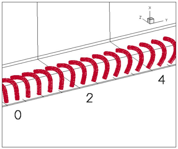
Final synchronized set of a linear array of cilia.

The mechanism of formation for a metachronal wave is important from a physiological point of view. Uncoordinated cilia motion is often observed in diseased states. The efficiency of transporting pathogens out of the lung is markedly increased when cilia beat together in a coordinated fashion. Elucidating the precise mechanism by which metachronal waves form and break down is useful in devising treatments.

6. Conclusions

A computational procedure for simulating the three-dimensional problem of entrainment of airway surface liquid by the motion of cilia has been presented. A realistic model of the internal elastic behavior of the cilium axo-neme has been introduced based upon a finite element model composed of large-deflection beams and elastic springs. The cilia interact with a two-layer model of the airway surface liquid consisting of a Newtonian periciliary layer and a viscoelastic mucus layer. The large number of cilia involved in a realistic simulation leads to considerable computational expense. However the model is naturally parallelized due to the use of individual body-fitted grids around each cilium that communicate through a background Cartesian grid using an overlapping grid technique. Results for a representative configuration of several cilia have been presented that provide evidence for a hydrodynamic origin to observed cilia metachronal wave patterns.

Several aspects of the model are open to criticism. There is uncertainty as to the mechanical characterization of the components of the biological system. The most important gap in the model is the ad hoc nature of the dynein force model. Full comparison of real microtubule bending motion with the beam model adopted here is not yet available. These points are under active investigation and will be addressed in future work. It is of significant physiological interest though that a metachronal wave in a row of cilia was obtained from tuning of the dynein forces in each cilium. This suggests that for normal cilium axonemes, synchronization between adjacent cilia occur naturally as a result of hydrodynamic interactions. Furthermore, computational simulation of a large enough number of cilia to be physiologically relevant has been shown to be possible and can be used as an additional tool that constrains parameters characterizing the biological system.

Appendix A. Stiffness matrices for beam element

The results of Felippa [11] are reproduced here for completeness. In-plane bending is assumed: M = M_B, M_N = M_T = 0, V_B = 0. The general displacement, force vectors at node i reduce to

$$U_i={\left[u_i{v}_i{\gamma }_i\right]}^{\mathrm{T}},F_i={\left[V_{T,i}{V}_{N,i}{M}_{B,i}\right]}^{\mathrm{T}}.$$

The shear distortion is θ = ψ - γ with γ the cross-section rotation and ψ the longitudinal axis rotation. The element longitudinal axis is at angle φ with respect to the global x-axis. Let ω = γ + φ and s = sin(ω), c = cos(ω) at the element midpoint. L₀, A₀, I₀ are the beam length, area, moment of inertia in the reference state. Let e = Lcos (γ - ψ)/L₀ - 1 with L the deformed length, a₁ = 1 + e.

The material stiffness matrix is

$$K_M=K_M^a+K_M^b+K_M^s.$$

The axial stiffness matrix is

$$K_M^a=\frac{EA}{L_0}\left[\begin{array}{cccccc}\hfill c^2\hfill & \hfill cs\hfill & \hfill -c\theta L_0∕2\hfill & \hfill -c^2\hfill & \hfill -cs\hfill & \hfill -c\theta L_0∕2\hfill \\ \hfill \hfill & \hfill s^2\hfill & \hfill -\theta L_{0}s∕2\hfill & \hfill -cs\hfill & \hfill -s^2\hfill & \hfill -\theta L_{0}s∕2\hfill \\ \hfill \hfill & \hfill \hfill & \hfill {\theta }^2{L}_0^2∕4\hfill & \hfill c\theta L_0∕2\hfill & \hfill \theta L_{0}s∕2\hfill & \hfill {\theta }^2{L}_0^2∕4\hfill \\ \hfill \hfill & \hfill \hfill & \hfill \hfill & \hfill c^2\hfill & \hfill cs\hfill & \hfill c\theta L_0∕2\hfill \\ \hfill \hfill & \hfill \hfill & \hfill \hfill & \hfill \hfill & \hfill s^2\hfill & \hfill c\theta L_0∕2\hfill \\ \hfill \hfill & \hfill \hfill & \hfill \hfill & \hfill \hfill & \hfill \hfill & \hfill {\theta }^2{L}_0^2∕4\hfill \end{array}\right].$$

The matrix is symmetric hence entries beneath the diagonal are not repeated. The bending stiffness matrix is

$$K_M^b=\frac{E{I}_0}{L_0}\left[\begin{array}{cccccc}\hfill 0\hfill & \hfill 0\hfill & \hfill 0\hfill & \hfill 0\hfill & \hfill 0\hfill & \hfill 0\hfill \\ \hfill 0\hfill & \hfill 0\hfill & \hfill 0\hfill & \hfill 0\hfill & \hfill 0\hfill & \hfill 0\hfill \\ \hfill 0\hfill & \hfill 0\hfill & \hfill 1\hfill & \hfill 0\hfill & \hfill 0\hfill & \hfill -1\hfill \\ \hfill 0\hfill & \hfill 0\hfill & \hfill 0\hfill & \hfill 0\hfill & \hfill 0\hfill & \hfill 0\hfill \\ \hfill 0\hfill & \hfill 0\hfill & \hfill 0\hfill & \hfill 0\hfill & \hfill 0\hfill & \hfill 0\hfill \\ \hfill 0\hfill & \hfill 0\hfill & \hfill -1\hfill & \hfill 0\hfill & \hfill 0\hfill & \hfill 1\hfill \end{array}\right].$$

The symmetric shear stiffness matrix is

$$K_M^s=\frac{G{A}_0}{L_0}\left[\begin{array}{cccccc}\hfill s^2\hfill & \hfill -cs\hfill & \hfill -a_1{L}_{0}s∕2\hfill & \hfill -s^2\hfill & \hfill cs\hfill & \hfill -a_1{L}_{0}s∕2\hfill \\ \hfill \hfill & \hfill c^2\hfill & \hfill c{a}_1{L}_0∕2\hfill & \hfill cs\hfill & \hfill -c^2\hfill & \hfill c{a}_1{L}_0∕2\hfill \\ \hfill \hfill & \hfill \hfill & \hfill a_1^2{L}_0^2∕4\hfill & \hfill a_{1}s{L}_0∕2\hfill & \hfill -c{a}_1{L}_0∕2\hfill & \hfill a_1^2{L}_0^2∕4\hfill \\ \hfill \hfill & \hfill \hfill & \hfill \hfill & \hfill s^2\hfill & \hfill -cs\hfill & \hfill a_{1}s{L}_0∕2\hfill \\ \hfill \hfill & \hfill \hfill & \hfill \hfill & \hfill \hfill & \hfill c^2\hfill & \hfill -c{a}_1{L}_0∕2\hfill \\ \hfill \hfill & \hfill \hfill & \hfill \hfill & \hfill \hfill & \hfill \hfill & \hfill a_1^2{L}_0^2∕4\hfill \end{array}\right].$$

The residual bending flexibility substitution is

$$G{A}_0\leftarrow 12E{I}_0∕L_0^2.$$

The geometric stiffness matrix is

$$K_G=K_{GN}+K_{GV}$$

with

$$K_{GN}=\frac{V_{T,m}}{2}\left[\begin{array}{cccccc}\hfill 0\hfill & \hfill 0\hfill & \hfill s\hfill & \hfill 0\hfill & \hfill 0\hfill & \hfill s\hfill \\ \hfill \hfill & \hfill 0\hfill & \hfill -c\hfill & \hfill 0\hfill & \hfill 0\hfill & \hfill -c\hfill \\ \hfill \hfill & \hfill \hfill & \hfill -a_1{L}_0∕2\hfill & \hfill -s\hfill & \hfill c\hfill & \hfill -a_1{L}_0∕2\hfill \\ \hfill \hfill & \hfill \hfill & \hfill \hfill & \hfill 0\hfill & \hfill 0\hfill & \hfill -s\hfill \\ \hfill \hfill & \hfill \hfill & \hfill \hfill & \hfill \hfill & \hfill 0\hfill & \hfill c\hfill \\ \hfill \hfill & \hfill \hfill & \hfill \hfill & \hfill \hfill & \hfill \hfill & \hfill -a_1{L}_0∕2\hfill \end{array}\right]$$

and

$$K_{GV}=\frac{V_{N,m}}{2}\left[\begin{array}{cccccc}\hfill 0\hfill & \hfill 0\hfill & \hfill c\hfill & \hfill 0\hfill & \hfill 0\hfill & \hfill c\hfill \\ \hfill \hfill & \hfill 0\hfill & \hfill s\hfill & \hfill 0\hfill & \hfill 0\hfill & \hfill s\hfill \\ \hfill \hfill & \hfill \hfill & \hfill -\theta L_0∕2\hfill & \hfill -c\hfill & \hfill -s\hfill & \hfill -\theta L_0∕2\hfill \\ \hfill \hfill & \hfill \hfill & \hfill \hfill & \hfill 0\hfill & \hfill 0\hfill & \hfill -c\hfill \\ \hfill \hfill & \hfill \hfill & \hfill \hfill & \hfill \hfill & \hfill 0\hfill & \hfill -s\hfill \\ \hfill \hfill & \hfill \hfill & \hfill \hfill & \hfill \hfill & \hfill \hfill & \hfill -\theta L_0∕2\hfill \end{array}\right].$$

Both K_GN and K_GV are symmetric. V_T,m and V_N,m are the axial force and shear force evaluated at the element midpoint.

References

- [1].Alberts B, Johnson A, Lewis J, Raff M, Roberts K, Walter P. Molecular biology of the cell. Garland; 2002. [Google Scholar]
- [2].Bathe K-J. Finite element procedures. Prentice-Hall; 1996. [Google Scholar]
- [3].Bird R, Hassager O, Armstrong R, Curtiss C. Dynamics of polymericliquids. Wiley; 1987. [Google Scholar]
- [4].Blake J. Mechanics of muco-ciliary transport. IMA J Appl Math. 1984;32:69–87. [Google Scholar]
- [5].Brown DL, Cortez R, Minion ML. Accurate projection methods for the incompressible Navier-Stokes equations. J Comput Phys. 2001;168:464–99. [Google Scholar]
- [6].Craster R, Matar O. Surfactant transport on mucus films. J Fluid Mech. 2000;425:235–58. [Google Scholar]
- [7].Crivelli L, Felippa C. A three-dimensional non-linear timoshenko beam based upon core-congruential formulation. Int J Numer Methods Eng. 2005;36:3647–73. [Google Scholar]
- [8].Dillon RH, Fauci LJ, Omoto C. Mathematical modeling of axoneme mechanics and fluid dynamics in ciliary and sperm motility. Dyn Contin Discrete Impulsive Syst. 2003;10:745–57. [Google Scholar]
- [9].Evans E, Heinrich V, Ludwig F, Rawicz W. Dynamic tension spectroscopy and strength of biomembranes. Biophys J. 2003;85:2342–50. doi: 10.1016/s0006-3495(03)74658-x. [DOI] [PMC free article] [PubMed] [Google Scholar]
- [10].Felgner H, Frank R, Schiiwa M. Flexural rigidity of microtubules measured with the use of optical tweezers. J Cell Sci. 1996;109:509–16. doi: 10.1242/jcs.109.2.509. [DOI] [PubMed] [Google Scholar]
- [11].Felippa C. Nonlinear finite element methods - online lecture notes. 2004 http://caswww.colorado.edu/courses.d/NFEM.d/Home.html
- [12].Gittes F, Mickey B, Nettleton J, Howard J. Flexural rigidity of microtubules and actin filaments measured from thermal fluctuations in shape. J Cell Biol. 1993;120:932–4. doi: 10.1083/jcb.120.4.923. [DOI] [PMC free article] [PubMed] [Google Scholar]
- [13].Grmela M, Ottinger H. Dynamics and thermodynamics of complex fluids. i. development of a general formalism. Phys Rev E. 1997;56:6620–32. [Google Scholar]
- [14].Grotberg J. Respiratory fluid mechanics and transport processes. Ann Rev Biomed Eng. 2001;24:421–57. doi: 10.1146/annurev.bioeng.3.1.421. [DOI] [PubMed] [Google Scholar]
- [15].Gueron S, Levit-Gurevich N, Blum J. Cilia internal mechanism and metachronal coordination as the result of hydrodynamical coupling. Proc Natl Acad Sci. 1997;94:6001–6. doi: 10.1073/pnas.94.12.6001. [DOI] [PMC free article] [PubMed] [Google Scholar]
- [16].Hughes T. Finite element method. Prentice-Hall; 1987. [Google Scholar]
- [17].Kirkham S, Sheehan JK, Knight D, Richardson PS, Thornton DJ. Heterogeneity of airways mucus: variations in the amounts and glycoforms of the major oligomeric mucins muc5ac and muc5b. Biochem J. 2002;361:537–46. doi: 10.1042/0264-6021:3610537. [DOI] [PMC free article] [PubMed] [Google Scholar]
- [18].LeVeque R. Wave propagation algorithms for multidimensional hyperbolic systems. J Comput Phys. 1997;131:327–53. [Google Scholar]
- [19].Lindeman CB. A geometric clutch hypothesis to explain oscillations of the axoneme of cilia and flagella. J Theor Biol. 1994;168:175–89. [Google Scholar]
- [20].MacNeal RH. A simple quadrilateral shell element. Comp Struct. 1978;8:175–83. [Google Scholar]
- [21].Matsui H, Randell SH, Peretti SW, Davis CW, Boucher RC. Coordinated clearance of periciliary liquid and mucus from airway surfaces. J Clin Invest. 1998;102:1125–31. doi: 10.1172/JCI2687. [DOI] [PMC free article] [PubMed] [Google Scholar]
- [22].Mayo A. The fast solution of Poisson’s and the biharmonic equations on irregular regions. SIAM J Numer Anal. 1984;21:285–99. [Google Scholar]
- [23].Minoura I, Yagi T, Kamiya R. Direct measurement of inter-doublet elasticity in flagellar axonemes. Cell Struct Funct. 1999;24:27–33. doi: 10.1247/csf.24.27. [DOI] [PubMed] [Google Scholar]
- [24].Mitran S, Fricks J, Elston T. A random-walker model of cilium axoneme forcing by dynein molecules, in preparation
- [25].Olson G, Linck R. Observations of the structural components of flagellar axonemes and central pair microtubules from rat sperm. J Ultrastruct Res. 1977;61:21–43. doi: 10.1016/s0022-5320(77)90004-1. [DOI] [PubMed] [Google Scholar]
- [26].Ottinger H, Grmela M. Dynamics and thermodynamics of complex fluids. II. illustrations of a general formalism. Phys Rev E. 1997;56:6633–55. [Google Scholar]
- [27].Pamploni F, Lattanzi G, Jonas A, Surrey T, Frey E, Florin E. Thermal fluctuations of grafted microtubules provide evidence of a length-dependent persistence length. Proc Natl Acad Sci USA. 2006;103:10248. doi: 10.1073/pnas.0603931103. [DOI] [PMC free article] [PubMed] [Google Scholar]
- [28].Kirkham S, Sheehan JK, Knight D, Richardson PS, Thornton DJ. Heterogeneity of airways mucus: variations in the amounts and glycoforms of the major oligomeric mucins muc5ac and muc5b. Biochemical Journal. 2002;361:537–46. doi: 10.1042/0264-6021:3610537. [DOI] [PMC free article] [PubMed] [Google Scholar]
- [29].Sears P, Davis W. private communication
- [30].Shingyoji C, Higuchi H, Yoshimura M, Katayama E, Yanagida T. Dynein arms are oscillating force generators. Nature. 1998;393:711–4. doi: 10.1038/31520. [DOI] [PubMed] [Google Scholar]
- [31].Silderberg A. Biorheological matching, mucociliary interaction and epithelial clearance. Biorheology. 1983;20:215–22. doi: 10.3233/bir-1983-20211. [DOI] [PubMed] [Google Scholar]
- [32].Sleigh MA. Coordinated clearance of periciliary liquid and mucus from airway surfaces. In: Sleigh MA, editor. Cilia and flagella. Academic Press; 1974. pp. 287–304. [Google Scholar]
- [33].Takahashi K, Shingyoji C, Kamimura S. Symp Soc Exp Biol. 1982;35:159–77. [PubMed] [Google Scholar]
- [34].Tarran R, Button B, Boucher R. Regulation of normal and cystic fibrosis airway surface liquid volume by phasic shear stress. Ann Rev Physiol. 2006;68:543–61. doi: 10.1146/annurev.physiol.68.072304.112754. [DOI] [PubMed] [Google Scholar]
- [35].Wang C, Liu J-G. Convergence of gauge method for incompressible flow. Math Comput. 2000;69:1385–407. [Google Scholar]
- [36].Widdicombe J, Widdicombe J. Regulation of human airway surface liquid. Respiration Physiol. 1995;99:3–12. doi: 10.1016/0034-5687(94)00095-h. [DOI] [PubMed] [Google Scholar]
- [37].Xie X, Pasquali M. A new, convenient way of imposing open-flow boundary conditions in two- and three-dimensional viscoelastic flows. J Theor Biol. 1994;168:175–89. [Google Scholar]
- [38].Xu W, Mulhern P, Blackford B, Jericho M, Firtel M, Beveridge T. Modeling and measuring the elastic properties of an archael surface, the sheath of methanospirillum hungatei, and the implication for methane production. J Bacteriol. 1996;178:3106–12. doi: 10.1128/jb.178.11.3106-3112.1996. [DOI] [PMC free article] [PubMed] [Google Scholar]