Studying visual search using systems factorial methodology with target–distractor similarity as the factor

Abstract

Systems factorial technology (SFT) is a theory-driven set of methodologies oriented toward identification of basic mechanisms, such as parallel versus serial processing, of perception and cognition. Studies employing SFT in visual search with small display sizes have repeatedly shown decisive evidence for parallel processing. The first strong evidence for serial processing was recently found in short-term memory search, using target–distractor (T–D) similarity as a key experimental variable (Townsend & Fifić, 2004). One of the major goals of the present study was to employ T–D similarity in visual search to learn whether this mode of manipulating processing speed would affect the parallel versus serial issue in that domain. The result was a surprising and regular departure from ordinary parallel or serial processing. The most plausible account at present relies on the notion of positively interacting parallel channels.

Walking into a café, you are looking for the familiar face of an old colleague with whom you have set an appointment. Doing so, you are engaged in a visual search for a target (your friend's face) among distractors (other people's faces). Are you more prone to quickly find her when the café is half empty than when it is crowded? Would certain properties, such as red hair, make her more likely to be detected? Similar themes arise when one is scanning a newspaper for words or topics of interest or even scrutinizing a face for a birthmark. The nature of visual search and the factors affecting the speed of processing have been extensively studied over the past half-century. A number of models have been put forth to explain how response times (RTs) are influenced by various stimuli and experimental conditions (Bundesen, 1990; Duncan & Humphreys, 1989; Palmer, Verghese, & Pavel, 2000; Treisman & Sato, 1990; Wenger & Townsend, 2006; Wolfe, 1994).

An especially intriguing question is that of processing architecture.¹ In the café, can we simultaneously process all faces (parallel processing), or is it necessary to process one face at a time (serial processing), until we recognize our friend? Is some kind of more complicated set of processes involved? Although this has been an issue of concern since the 19th century, and intensive experimental and theoretical researches on such issues have continued for several decades, decisive resolution has been hard to come by.

The most common experimental approach since the 1960s has been to manipulate the number of search objects (workload) and measure RTs (for memory search, see Sternberg, 1966; for visual search, see Atkinson, Holmgren, & Juola, 1969, and Egeth, 1966). For example, when participants search for a single visual target among distractors that are highly similar to the target, mean RTs can increase in a linear fashion as a function of workload, thus suggesting serial processing (e.g., Atkinson et al., 1969; Townsend & Roos, 1973; Treisman & Gelade, 1980; Wolfe, Cave, & Franzel, 1989). On the other hand, under certain conditions and even with manipulation of workload, participants can exhibit rapid RTs or patterns of accuracy that are more compatible with parallel processing (e.g., Bacon & Egeth, 1994; Bundesen, 1990; Folk & Remington, 1998; Palmer et al., 2000; Pashler & Harris, 2001; Thornton & Gilden, 2007; Wenger & Townsend, 2006).

Unfortunately, there is a marked asymmetry in the use of workload as an independent variable to assess architecture. On the positive side, when RT decreases or, in some cases, remains roughly constant with an increase in workload, models based on parallel processing are virtually the only viable type of alternative. The reason for the conclusiveness is that serial models would have to increase their processing speed in an outlandish way in order to make such predictions. Yet, in scores of experiments utilizing a single target embedded in a set of distractors (a few have been indicated just above), RT increases with workload, and here the inference is decidedly more ambiguous. The problem is that quite natural parallel models whose channels² become less efficient as workload increases can make predictions identical to those of serial models (e.g., Townsend, 1969, 1971, 1972; Townsend & Ashby, 1983); this is the well-known model-mimicking dilemma.³

There is a more powerful theory-driven methodology that has evolved over the past several decades that is able to avoid most, if not all, model-mimicking challenges and certainly those associated with the architecture–capacity confounding. This approach grew out of Sternberg's additive factors method, which allowed assessment of the hypothesis of serial processing. We will explain the methodology further below, but suffice it to say for now that the prime logic is that experimental factors can be found that selectively slow down or speed up separate subprocesses or subsystems in the overall processing network (the so-called postulate of selective influence; Ashby & Townsend, 1980; Dzhafarov, 1999; Egeth & Dagenbach, 1991; Sternberg, 1969; Townsend, 1984; Townsend & Thomas, 1994). These methods were subsequently generalized to permit identification not only of parallel processing, but also of other feedforward systems of rather surprising complexity (Schweickert, 1978; Schweickert, Giorgini, & Dzhafarov, 2000; Schweickert & Townsend, 1989; Townsend & Ashby, 1983).

We have employed this methodology, now often referred to globally as systems factorial technology (SFT), to investigate visual search with a small workload in a number of important contexts: in binocularly present dots (e.g., Hughes & Townsend, 1998; Townsend & Nozawa, 1988, 1995); realistic facial feature identification (e.g., Fifić, 2006; Wenger & Townsend, 2001), emotional facial feature perception (e.g., Innes-Ker, 2003), short-term memory search (e.g., Townsend & Fifić, 2004), and nonface meaningful and meaningless objects (e.g., Wenger & Townsend, 2001). In all the visual search situations, the results have always strongly supported parallel processing. All these experiments utilized some type of salience manipulation as a selective experimental factor. And none of them involved letters or words as stimuli. In contrast, in a short-term memory search experiment with word-like stimuli (Townsend & Fifić, 2004), it was necessary to engage a different type of factor: the similarity of distractors to the target. That study showed marked individual differences, with some observers revealing serial and others parallel processing.

As has been noted, although the factorial approach in general can assess complex networks, our data have so far corroborated simple parallel or, sometimes in memory search, serial processing. We shall refer to these as single-stage models, since the main search mechanisms are confined to a single stage in the overall cognitive-processing chain. Yet a highly popular class of models is based on three stages of processing: a very efficient parallel early stage, followed by a selection process that sends certain items to a third, limited-capacity, usually serial, later stage used to search through more difficult items (Sagi & Julesz, 1985; Treisman & Gelade, 1980; Treisman & Sato, 1990; Wolfe, 1994). Although there appear to be many directions one could take in extracting predictions from such multistage models, we will begin to probe some apparently natural, if simplified, possibilities.

The present study was intended first to expand the purview of SFT to meaningless word-like or letter stimuli. Second, we employed similarity of distractors to the target as a selective factor, as was done in the short-term memory study (Townsend & Fifić, 2004), but not heretofore in visual search. Third, we wished to manipulate the complexity of the items in order to explore its effect on architecture. Would the experimental evidence again provide uniform support for parallel processing? How would our simple extensions of the popular three-stage models fare? As will be seen, the results deviated radically from earlier findings.

Factorial Technology Tests of Parallel Versus Serial Systems

SFT is a theory-driven experimental methodology that unveils a taxonomy of four critical characteristics of the cognitive system under study: architecture (serial vs. parallel), stopping rule (exhaustive vs. minimum time), workload capacity (limited, unlimited, or super), and channel independence. The first three are directly tested by our RT methodology. Independence can only be indirectly assessed, although channel dependencies can affect capacity (e.g., Townsend & Wenger, 2004b). To directly test for independence, the investigator needs the accuracy-based analyses afforded by general recognition theory (e.g., Ashby & Townsend, 1986). Architecture and stopping rule are the primary characteristics targeted in this study, but we will see that capacity and, possibly, channel dependencies may be implicated in the interpretations.

It is important to observe that all of our assessment procedures are distribution and parameter free. Most experimentation pursues tests of qualitative predictions (e.g., Group A is faster than Group B) of verbally founded predictions. More rigorous modeling typically tests mathematical models that are based on specific probability functions (normal, Gaussian, gamma, etc.) by estimating the parameters that provide a “best” fit to the data and then, sometimes, determining whether the fit is statistically significant or not. If it is, the model is said to be supported by the data; if not, the model is said to be falsified. In the SFT approach, powerful qualitative predictions are made that, if wrong, can falsify huge classes of models—for instance, the set of all mathematical functions that obey the prime psychological assumptions. If confirmed (not falsified), more specific, parameter-based models can be explored.

As was intimated earlier, SFT analysis is based on a factorial manipulation of at least two factors with two levels, and it utilizes two main statistics: the mean interaction contrast (MIC; Ashby & Townsend, 1980; Schweickert, 1978; Sternberg, 1969) and the survivor interaction contrast (SIC). The latter extension makes use of data at the distributional level, rather than means, and therefore permits analysis at a more powerful and detailed level (Townsend, 1990; Townsend & Nozawa, 1988, 1995; for extension to complex networks, see Schweickert et al., 2000).

The MIC statistic describes the interaction between the mean RTs of two factors with two levels each and can be presented as follows:

$$\begin{array}{cc}\hfill \mathrm{MIC}& =\left({\mathrm{RT}}_{\mathrm{LL}}-{\mathrm{RT}}_{\mathrm{LH}}\right)-\left({\mathrm{RT}}_{\mathrm{HL}}-{\mathrm{RT}}_{\mathrm{HH}}\right)\hfill \\ \hfill & ={\mathrm{RT}}_{\mathrm{LL}}-{\mathrm{RT}}_{\mathrm{LH}}-{\mathrm{RT}}_{\mathrm{HL}}-{\mathrm{RT}}_{\mathrm{HH}}.\hfill \end{array}$$ (1)

There are two subscript letters; the first denotes the level of the first factor (H = high, L = low), and the second indicates the level of the second factor. Note that MIC gives the difference between differences, which is literally the definition of interaction. MIC = 0 indicates that the effect of one factor on processing latency is exactly the same, whether the level of the other factor is L or H. Conversely, if two factors interact, manipulating the salience of one factor would yield different effects depending on the level of the other factor; hence, MIC ≠ 0. Underadditive interaction, or MIC < 0, is a typical prediction of parallel exhaustive processing, whereas additivity, or MIC = 0, is associated with serial exhaustive processing (Townsend & Ashby, 1983; Townsend & Nozawa, 1995).

The survivor interaction contrast function (SIC) is defined as

$$\mathrm{SIC}\left(t\right)=\left[S_{\mathrm{LL}}\left(t\right)-S_{\mathrm{LH}}\left(t\right)\right]-\left[S_{\mathrm{HL}}\left(t\right)-S_{\mathrm{HH}}\left(t\right)\right],$$ (2)

where S(t) denotes the RT survivor function. In brief, to calculate the SIC, we divide the time scale into bins (say, of 10 msec each) and calculate the proportion of responses given within each time bin to produce an approximation to the density function, f(t), and the cumulative probability function F(t). That is, F(t) is equal to the probability that RT is less than or equal to t. The survivor function, S(t), is the complement of the cumulative probability function [1 – F(t)] and tells us the probability that the process under study finishes later than time t. To produce the SIC, one calculates the difference between differences of the survivor functions of the four corresponding factorial conditions the way it is derived for the means, but does so for every bin of time.

Note that this statistic produces an entire function across the values of observed RTs. Furthermore, there is a specific signature of each architecture and stopping rule, with respect to the shape of the SIC function (Townsend & Nozawa, 1988, 1995). For example, the SIC function for a parallel exhaustive model is negative for all time. Perhaps surprisingly, the serial exhaustive processing SIC function is not identically equal to 0 but, rather, is first negative and then positive (see Figure 1). Furthermore, the positive area is predicted to be identical to the negative area. Because this study will, as in Townsend and Fifić (2004), analyze only target-absent trials, the focus will be on the exhaustive (i.e., and) stopping rule.⁴ MIC and SIC predictions for serial exhaustive and parallel exhaustive models are presented in Figure 1. Although the MIC is not nearly as diagnostic as the SIC, it both reinforces the SIC results and provides a means of statistically assessing any interactions associated with the SIC function.⁵

Figure 1.

The predicted signatures of serial exhaustive (left) and parallel exhaustive (right) processing revealed by systems factorial technology analysis. The expected survivor interaction contrast (SIC) as a function of time is presented for each model. The predicted factorial interaction on the means (MIC) is boxed inside each figure. Both SIC functions are calculated without an inclusion of a residual time (processing time that is due to nonsystematic variability—for example, a motor response).

The topic of workload capacity plays a relatively minor role here, but it will be required in some of the discussion. Basically, we measure capacity by comparing the actual efficiency when, say, n channels are operating with that predicted by a regular, independent (unlimited capacity, by definition) parallel-processing model. This is accomplished by taking the RT distribution at n = 1 and compounding it in the way predicted by the regular parallel model. This computation creates a capacity function over time. If the actual result is identical to the regular parallel predictions, we call the underlying mechanism (be it serial, parallel, or hybrid) unlimited capacity. If the speed is less than that predicted by the regular parallel model, we say it is limited capacity. If it somehow supersedes the regular parallel prediction, it is called super capacity. In particular, we have repeatedly found that perception of good, configural visual objects can, in certain circumstances, elicit super capacity or, contrarily, lead to limited capacity (e.g., Townsend & Wenger, 2004b; Wenger & Townsend, 2006).

Before ending this section, we need to mention two important nonindependent parallel channels models. One rather distinct type, coactive parallel processing, does away with the assumption that separate decisions (e.g., recognition of an item) are made in the distinct channels. Rather, it is assumed that the multiple-channels pool—for instance, add—their activations together in a final single mutual conduit. The activation level then is continuously compared with a single decision criterion. This idea and its name stem from J. Miller's work on better-than-regular parallel processing (e.g., Miller, 1982; for mathematical renditions of such processing, see Colonius & Townsend, 1997; Diederich & Colonius, 1991). Townsend and Nozawa (1995) proved that a large class of coactive models, based on general counting processes (whose individual channels do not slow down with increased workload and that are summed in a subsequent conduit), inevitably predict super capacity. In fact, the capacity is sufficiently super that Miller's (1982) well-known inequality must be violated. The latter authors also showed that there is a special case of coactive models, based on Poisson counting channels, that predict SIC curves that are S-shaped like exhaustive serial models but whose early negative parts are small, in contrast to the serial models.

A rather different variety of nonindependent parallel models simply assume that the parallel channels interact in a mutually facilitatory manner but still possess decision thresholds within each channel (Mordkoff & Yantis, 1991; Townsend & Wenger, 2004b). We know that this class of models is quite broad, including true coactive models as a special case (Colonius & Townsend, 1997). Hence, they must be able to predict S-shaped SIC functions with total positive area, but we do not know whether this can be accomplished in a psychologically interesting way. These mutually facilitatory channel models are also capable of predicting supercapacity findings (Townsend & Wenger, 2004b). We shall indicate some recent theoretical results with such models in the General Discussion section.

The factorial combination of (item position) × (target–distractor visual dissimilarity) provides for the tests of system architecture. When factorial tests are applied, the simple, single-stage models predict the shape of the SIC function to be consistent with the signature predicted by either a serial exhaustive or a parallel exhaustive system (Figure 1). The MIC value should, correspondingly, reveal either additivity or underadditivity.

A number of alternative varieties of process architecture, including some special simple types of three-stage models, are assayed. It turns out that the simplest displays, where the stimuli consisted of a single letter (C = 1), afford what, at first glance, looks like standard serial processing. However, when the nonsignificant interaction trend in C = 1 is combined with the intriguing results from the more complex conditions (C = 2, 3), we are forced to move to more intricate single-stage models for the overall corpus of data. Potentially, some multistage models may also account for the data. Naturally, multistage models in general form a huge class of alternatives, and it is challenging to pinpoint detailed predictions in the general case. Certain natural, if quite simple, special types of multistage models can be decisively falsified.

EXPERIMENT 1

Method

Participants

Four participants, 2 females and 2 males, were paid for their participation. All had normal or corrected-to-normal vision. They were all native speakers of Serbian and familiar with the Cyrillic alphabet.

Materials

The stimuli were letter strings made up of Cyrillic letters. In a visual search task, a target is presented before a set of test items, which constitute a test display. The task was to search across test items for a target presence. Test items that are not identical to a target are called distractors. We manipulated the visual complexity of the stimuli and the degree of visual dissimilarity between the target and each of the test items. Note that we use the term dissimilarity, rather than similarity, in order to be consistent with previous work (Townsend & Fifić, 2004). Table 1 presents examples of actual target-absent trials for different levels of item complexity (C = 1, 2, 3) and different levels of target-to-test item dissimilarity (HH, HL, LH, and LL, where H stands for high dissimilarity and L for low dissimilarity), in Experiment 1.

Table 1.

Examples of the Actual Target-Absent Trials for Different Item Complexity Levels (C = 1, 2, 3) for Curved and Straight-Line Letters in Experiment 1

Factorial Condition	Target	Test (Display) Items
C = 1
LL	Б	З, B
	П	H, П
HL	З	Ш, B
	H	З, П
LH	H	П B
	B	З, H
HH	Ш	B, Б
	Б	П, Ш
C = 2
LL	БB	БЗ, BЗ
	ПШ	ПH, ШП
HL	ЗB	ШП, BЗ
	HШ	BЗ, ПH
LH	HШ	ШП BЗ
	ЗB	BЗ, ПH
HH	ПШ	BЗ, BБ
	BБ	HП, HШ
C = 3
LL	БBЗ	БЗB, BЗБ
	ПШH	ПHШ, ШПH
HL	ЗBБ	ШПH, BЗБ
	HШП	BЗБ, ПHШ
LH	HШП	ШПH, BЗБ
	ЗBБ	BЗБ, ПHШ
HH	ПШH	BЗБ, BБЗ
	БBЗ	HПШ, HШП

Note—The factorial condition indicates the degree of dissimilarity (L for low, H for high) between each test item and the target item. For example, HL denotes a trial on which the left test item was highly dissimilar to the target, whereas the right test item shared low dissimilarity with the target.

We manipulated the visual complexity of the letter-string stimuli by varying the number of letters that made up a single item (1, 2, or 3). For a given level of complexity, the number of letters in the target item was identical to the number of letters in each test item.

To manipulate the degree of visual dissimilarity, we employed two sets of letters: letters with curved features (Б, В, З) and letters with straight-line features (П, Ш, Н). Note that the items within each group were mutually confusable; that is, each of the items was relatively similar to other members of its own group but relatively dissimilar to members of the other group. We then generated different dissimilarity levels by constructing the target and test items from letters drawn either from the same group or from different groups. In Appendix A we test and demonstrate how this technique directly affects the perceptual dissimilarity between items.

To generate the factorial conditions necessary for the MIC and SIC architecture tests, we factorially combined the position of the test item and its visual dissimilarity to the target item. Four orthogonal conditions were thereby generated; HH, HL, LH, and LL, where the position of the letter denotes the position of the relevant test item with respect to the fixation point (left or right). So, HL indicates that two test items were presented; the left was highly dissimilar to the target, whereas the right item possessed low dissimilarity to the target. Since we used two sets of letters, curved and straight, the HL display may represent a case in which the target and the right test item were made of, say, curved letters, whereas the left test item was made of straight letters. Alternatively, on HH trials, when the target was made of curved letters, both test items were made of straight-line letters, and vice versa. Observe that in the HH display, the two test items would be relatively similar to each other, whereas in the HL display, they would be dissimilar to each other (Table 1).

Design and Procedure

The participants were tested individually in a dimly lit room. The two test items in the most complex condition (C = 3, with the widest stimuli) spanned 5 cm horizontally. At a viewing distance of 1.7 m from the computer screen, this width corresponds to a visual angle of 1.86°, well within the fovea. A test display was presented until a response was made, and then a new trial began.

Each trial started with a fixation point that appeared for 700 msec and a low-pitch warning tone of 1,000 msec, followed by the presentation of the target item for 400 msec. Then a mask was presented for 130 msec, followed by two crosshairs that indicated the positions of the two upcoming test items. A high-pitch warning tone was then played for 700 msec, followed by the presentation of the test items. The test display remained on the screen until a response was given.⁶

Half of the trials were target present, and half were target absent. On each trial, the participant had to indicate whether or not the target item appeared on the test display by pressing either the left or the right mouse key with his/her corresponding index finger. RTs were recorded from the onset of the test display, up to the time of the response. The participants were asked to respond both quickly and accurately.

Each participant performed on 30 blocks of 128 trials each, each block on a different day. The order of trials was randomized within blocks. The complexity of the presented items (i.e., the number of letters: C = 1, 2, or 3) was manipulated between blocks, whereas factorial combinations (HH, HL, LH, LL) varied within blocks. For each participant, the mean RT for each conjunction of item complexity and factorial combination was calculated from approximately 200 trials. We found this number of trials to be sufficient for testing models at the individual-participant level, both for the ANOVA and for calculating survivor functions.

Results

We analyzed data within individual participants. When the results exhibited a uniform pattern across participants, we also report group statistics.

We ran a one-way ANOVA on mean RT averaged over participants. We used the factor of the item complexity level (C = 1, 2, 3). The main effect of item complexity was significant [F(2,6) = 74.28, p < .01], showing a trend of increasing RTs with increasing complexity of the presented items (mean RT_C1 = 576 msec, SE = 26.37 msec; mean RT_C2 = 786 msec, SE = 57.89 msec; mean RT_C3 = 924 msec, SE = 54.37 msec).

We performed a separate ANOVA for individual participants, where F₁ was defined as the visual dissimilarity between the left test item and the target (high or low). F₂ was similarly defined for the right test item. Together, F₁ and F₂ yielded four experimental conditions: HH, HL, LH, and LL. The F₁ × F₂ interaction indicated the significance of the observed MIC value.

Both main effects (F₁ and F₂) were significant at p < .01 in the higher item complexity conditions (C = 2, 3) for all the participants. For 3 out of the 4 participants, both main effects were significant in the single-letter presentation, C = 1 (Participant 1 exhibited a significant main effect for F₂ but not for F₁). Next, we will turn to an analysis of the results of the mean interaction contrast, MIC, and the survivor interaction contrast, SIC.

Mean and survivor interaction contrast functions

In Table 2, we present the interaction test on means (MIC) for each of the participants for different complexity levels. The results are remarkably uniform across participants. They all exhibited an overadditive MIC on the higher item complexity levels (C = 2, 3), and all of them, excluding Participant 1, exhibited an additive MIC on the lowest level of item complexity (C = 1; stimulus items that were made of one letter). Hence, additivity, which is associated with a serial exhaustive processing, was manifested by 3 out of the 4 participants in the C = 1 condition. Nonetheless, it is important that we note that the tendency of all the participants, even those in the C = 1 condition, was toward overadditivity, just not significantly so. Furthermore, it is evident that all the participants exhibited less overadditivity (i.e., smaller MIC values) in the C = 3 than in the C = 2 condition. That is, there is a nonmonotonicity with regard to how overadditivity acted as a function of complexity, first increasing, and then decreasing, with complexity.

Table 2.

Mean Interaction Contrast (MIC) Analysis of Experiment 1, Calculated Separately for Each Level of Item Complexity and for Each Participant

Participant	MIC (msec)	df	F	p	Power
C = 1 (One-Letter Target)
1	−41*	1, 558	3.85	.05	.50
2	12	1, 554	1.38	.24	.22
3	18	1, 553	0.97	.32	.17
4	16	1, 558	2.13	.14	.31
C = 2 (Two-Letter Target)
1	168**	1, 596	33.92	.00	1.00
2	133**	1, 593	43.25	.00	1.00
3	179**	1, 595	65.79	.00	1.00
4	140**	1, 596	36.20	.00	1.00
C = 3 (Three-Letter Target)
1	64*	1, 594	4.93	.03	.60
2	52	1, 589	3.53	.06	.47
3	98**	1, 584	12.56	.00	.94
4	96**	1, 590	12.88	.00	.95

Note—The MIC factors were the degree of visual dissimilarity between the target item and each of the test items. Since the main effects were significant for almost all cases, we present only the interaction contrast (but see the text for detailed information). df stands for degrees of freedom.

^*p < .05.

^**p < .01.

In Figure 2 we present graphically the MIC and SIC figures for the individual participants. The SIC functions are on the left, and the corresponding MIC figures are on the right. As the reader may note, most SIC functions exhibit an S-shape, which by itself is associated with serial exhaustive processing.⁷ However, concurring with the ANOVA results, for the C = 2 and 3 conditions, the summed areas of several SIC functions are significantly greater than zero, which is, of course, inconsistent with serial exhaustive processing. We will discuss this finding in the next section. As has been noted, a single exception is the data of Participant 1 from the C = 1 condition, who showed mainly a negative SIC (and demonstrated a consequent negative MIC value; see Table 2 and Figure 2), which is consistent with parallel exhaustive processing. However, this atypical result is disputable, given that one of the main effects (F₁) did not reach significance.⁸

Figure 2.

Systems factorial technology analysis of the data from Experiment 1 (only for the target-absent trials). The survivor interaction contrast (SIC) and the mean interaction contrast (MIC) are presented from left to right. Error bars around each mean represent the standard error statistic. Different participants are presented in different rows, and the figures are sorted by the item complexity level (C = 1, 2, 3).

Error analysis

The mean error level for target-absent trials, averaged across all participants, was 1.1%. No speed–accuracy trade-off was observed: Both mean RTs and mean errors increased across item complexity.

Discussion

The participants exhibited longer RTs when moving from item complexity C = 1 to more complex displays, C = 2 and C = 3. Both MIC and SIC patterns were consistent across participants. The SIC functions in the C = 2 and C = 3 conditions generally revealed an S-shape that roughly resembles the signature of serial exhaustive processing, and the C = 1 condition could be taken as indicative of serial processing, given that the MIC is nonsignificant. However, the positive portion of the curve was typically much larger than the negative portion for C > 1. Taken together with the nonsignificant trend in C = 1, the results suggest that overadditivity, not additivity or under-additivity (as in parallel exhaustive processing), was the modal characteristic of processing in this study.⁹

Furthermore, MIC increased from C = 1 to C = 2 and decreased from C = 2 to C = 3. However, it was still significant for most of the C = 3 participants. Does the shift from additive to overadditive MIC, as we vary the complexity of the visual display, indicate a qualitative change in the architecture (from serial to parallel)? To acquire an even more accurate answer, we conducted additional analyses on the trends of mean RTs over different item complexity levels, for distinct factorial conditions (see Appendix B for details).

These additional analyses revealed that RTs on different factorial conditions (HH, HL, LH, and LL) changed differently as a function of item complexity. RTs on LL and HH conditions increased in a concave down (negatively accelerated) fashion when item complexity was increased, whereas RTs on HL and LH conditions increased linearly. This differential change, as we increase the complexity of the presented items, leads to a change from additive to highly overadditive to low overadditive MIC that does not necessarily reflect a real change in the processing architecture.

One account of why the effect of item complexity on processing in the LL and HH conditions departs from its effect in the HL and LH conditions (in fact, on the overall mean RT patterns) is that, in accordance with Duncan and Humphreys (1989), visual search latencies are affected both by the target-to-distractor dissimilarity (i.e., the dissimilarity between the target and each of the test items, denoted earlier as T–D) and by the mutual similarity of distractors (denoted D–D). The two test items in the LL display are highly similar to each other, as are the test items in the HH display. In the HL (alternatively, LH) condition, on the other hand, the two test items are highly dissimilar to each other.

By increasing the complexity of items (as we increase the number of their constituting letters), we generally impair the visual search, but, in the HH and LL conditions, this effect may be countered by a relative facilitation due to the increased mutual similarity. In popular multistage models, this dynamic could be represented in an underlying selection process: When (two) distractor items are mutually similar, an efficient grouping process that can select them on the basis of a common property is activated. That grouping or scene segmentation process is a fast parallel process that is postulated in somewhat different ways in several theories: as feature inhibition (Treisman & Sato, 1990), as spreading suppression (Duncan & Humphreys, 1989), or as a complex network of several subnetworks that maintain efficient parsing of the visual scene (Grossberg, Mingolla, & Ross, 1994). When such a grouping process is deployed, higher efficiency of visual search is achieved, and overall mean RTs are shorter. To have an intuitive idea of how mutual similarity between test items may increase the efficiency of visual search, consider again the example provided at the beginning of the article: Looking for the familiar face of a friend in a crowded café may become much easier if all the other patrons are identical siblings.

It is worth noting that we observed the mean overadditivity in the more complex conditions (C = 2, 3) in an unpublished experiment that comprised several hundred trials per condition. The C = 1 condition offered ambiguous results and prompted the full-scale study presented here. In the C > 1 conditions, as in the present work, we consistently observed S-shaped SIC functions with a positive part larger then the negative one for different durations of display: from a limited duration of 300 msec to an “unlimited” duration (where the test items are displayed until a response is given). Although it could be expected that presenting a display for an unlimited duration would encourage serial processing (McElree & Carrasco, 1999; Zelinsky & Shein berg, 1997), the overadditive S-shaped SIC function—not predicted by serial processing—was consistently evident in both viewing conditions, limited and unlimited.

Previous visual search experiments conducted in our lab have yielded consistent evidence for parallelism. Perhaps the most obvious difference, apart from use of D–D similarity, in the present study was the employment of linguistic or alphabetic-related stimuli, as opposed to the nonalphabetic stimuli (dots, faces, etc.) employed in previous experiments. Experiment 2 was designed to investigate whether the overadditivity combined with S-shaped SIC curves could be associated with letter stimulus items, as opposed to our usual pictorial stimulus patterns—for instance, via reading habits. We therefore used meaningless visual patterns instead of letters in the next experiment. We employed only the single-item complexity level (C = 1), since it was the only condition so far to engage anything close to pure serial processing.

EXPERIMENT 2

Method

Participants

Four participants, 3 females and 1 male, were paid for their participation. All had normal or corrected-to-normal vision. The experiment was carried out at Indiana University, Bloomington.

Materials and Design

As stimuli, we used meaningless visual patterns taken from Microsoft's Windows standard fonts. The design was identical to that in the previous experiment, except that we used only the simplest level of item complexity, C = 1. Each participant performed in 10 blocks of 128 trials. Actual trials (i.e., target and test items) for each factorial condition are presented in Table 3.

Table 3.

Actual Trials in Experiment 2 for Different Factorial Conditions

Factorial Condition	Target	Test (Display) Items
C = 1
LL	∩	⊂, ∪
	▭	▭, ▭
HL	▭	⊂, ▭
	∩	▭, ∪
LH	∩	⊂, ▭
	▭	▭, ∪
HH	▭	⊂, ∪
	∪	▭, ▭

Note—Meaningless visual patterns were presented rather than letters, and only the simplest level of item complexity, C = 1, was used. As in Experiment 1, we were interested in the target-absent trials.

Results

We analyzed only the data from target-absent trials, for each participant, as noted, for a single-item complexity level (C = 1). We used the following ANOVA design: F₁ (low or high) × F₂ (low or high). The interaction of interest (MIC) and the main effects (F₁ and F₂) were defined in the same way as in the previous experiment. All the main effects were significant at p < .01. Table 4 reveals uniform results across participants: All of them exhibited overadditivity, as is evident from the positive values of the MIC, although for 2 of the participants, it was not statistically significant, as in the C = 1 condition in Experiment 1.

Table 4.

Mean Interaction Contrast (MIC) Analysis of Experiment 2, Calculated Separately for Each Participant

Participant	MIC (msec)	df	F	p	Power
1	49	1, 550	2.59	.11	.36
2	70*	1, 539	6.39	.01	.71
3	18	1, 547	2.13	.15	.31
4	22*	1, 550	4.32	.04	.55

Note—df stands for degrees of freedom.

^*p < .05.

^**p < .01.

Mean and survivor interaction contrast functions

In Figure 3, we present graphically the MIC and SIC figures for the individual participants. The SIC functions are presented on the left, and the corresponding MIC figures are on the right. All SIC functions exhibit the now- familiar S-shape, with the positive area being greater than the negative area.

Figure 3.

Systems factorial technology analysis of the data from Experiment 2 (only for the target-absent trials). The survivor interaction contrast (SIC) and the mean interaction contrast (MIC) are presented from left to right. Errors bars around each mean represent the standard error statistic. Different participants are presented in different rows.

Error analysis

The mean error rate for the target- absent trials was 2%. Participant 2 had 3.2% errors, whereas Participant 1 exhibited the lowest error rate, with 1.2%.

Discussion

All the participants exhibited S-shaped SIC functions. Two of the participants in Experiment 2 exhibited overadditive MIC, which is consistent with the MIC values observed in the higher complexity conditions (C = 2 and C = 3) in Experiment 1. The 2 other participants demonstrated positive yet nonsignificant MIC values, as in the nonsignificant trend in the C = 1 condition for the first experiment.

Experiment 2 assessed the hypothesis that relatively simple and nonlinguistic stimulus patterns would elicit pure seriality, as would be evidenced by MIC = 0. This expectation was not fulfilled. The results from Experiment 2 demonstrated that the overadditivity found in Experiment 1, and in unpublished experiments, likely was not caused by the linguistic nature of letter stimuli (for instance, by way of special “reading” subprocesses) or simply by the extra complexity associated with C = 2 or C = 3 versus C = 1.

GENERAL DISCUSSION AND INTERIM THEORETICAL CONCLUSIONS

The general goal of the present study was to further explore the type of architectures that are involved in various kinds of visual search, using SFT. Many studies in the visual search literature have argued for a serial process that is engaged somewhere in the visual system. Contemporary renditions on this theme often argue for a multistage model, containing an early parallel feature map, followed by a transport of complex and feature-conjoined stimuli (Treisman & Sato, 1990; Wolfe, 1994) to a subsequent third serial stage. Aware of the mimicking problem between parallel and serial architectures when RT increases with workload, some of those studies have postulated seriality simply as a convention.

We shall consider a small set of such models as candidates for our data below.

Yet, a number of studies using SFT over the past decade or so have shown that (at least for a small display size) manipulations of magnitude factors, such as clarity and brightness, provide unequivocal support for parallelism with stimuli as simple as dots and as complex as facial photographs (e.g., Hughes & Townsend, 1998; Townsend & Nozawa, 1995; Wenger & Townsend, 2001). Considering the complexity of the human neural and information-processing systems, it would be remarkable if every kind of search turned out to be more or less identical. Indeed, recent experiments in short-term memory search, which may have engaged verbal/phonemic facets, have revealed individual differences, with certain conditions and individuals evincing persuasive evidence for seriality, others for parallelism even when only two items are contained in the memory set (Townsend & Fifić, 2004).

Apart from the obvious experimental distinction between memory and visual search, the Townsend and Fifić (2004) memory search task employed T–D similarity as the architecture-detecting factor, a rather different manipulation from the variation of intensity or clarity that has commonly been used in visual search studies in which uniform support for parallelism has been found. Hence, it was desirable to investigate this novel factor within a visual, rather than a memory, search paradigm. In addition, with the exception of the recent Wenger and Townsend (2006) study, quasilinguistic stimuli have not been examined within our approach, and the latter experiments focused on workload and redundant signals manipulations (as did Thornton & Gilden, 2007), rather than a selective influence factorial design, as was the case here. The latter type of manipulation most directly measures capacity, but since the effects of increased workload vary with architecture, consistent findings across conditions can allow reasonably strong inferences concerning architecture. Wenger and Townsend's (2006) study showed broad support for parallel process in both words and faces, as well as unorganized letter strings and scrambled facial features. The Thornton and Gilden (2007) investigation, employing a wide variety of visual stimuli, obtained considerable evidence of parallel processing but also unearthed conditions in which serial processing was supported. In the present work, we wished to learn whether presenting letters versus nonletters would affect the processing mode in a visual search task under selective influence treatment. Finally, it was deemed important to assay how varying complexity might affect the identified architecture.

Within the SFT setting, we employed systems factorial tests at the distributional level, which are more powerful and detailed with regard to processing characteristics than the standard test of means (Townsend & Nozawa, 1988, 1995). We analyzed only responses on target-absent trials on which participants had to use an exhaustive stopping rule: In order to correctly reject two test items that were not the target item, both items had to be searched. Given an exhaustive stopping rule, the two main candidate architectures were the serial exhaustive and the parallel exhaustive models, which possess unique signatures. In serial exhaustive processing, MIC is predicted to be zero, and the SIC functions are S-shaped, with the negative area coming first and equal in size to the subsequently appearing positive area. In parallel exhaustive processing, the MIC is less than zero, and the SIC functions are predicted to be entirely less than zero (see Figure 1).

The participants in Experiment 1 were tested in several blocked item complexity conditions (item complexity refers to the number of letters in each item: one, two, or three). Overall, as complexity increased, responses were slower. Furthermore, almost all of the participants, in both experiments and across different conditions, exhibited an S-shaped SIC function, which is qualitatively similar to the signature of serial exhaustive processing. And the negative areas appeared first in time, just as was expected. Indeed, the MIC values were essentially zero in C = 1 conditions, as serial processing predicts. Nonetheless, the (C = 1) data indicated a trend toward overadditivity, although none of the participants exhibited statistical significance. When C > 1, the S-shaped SIC functions repeatedly exhibited positive areas greater than the negative areas, suggesting that something other than pure serial or parallel processing was taking place. And the MIC statistics indicated significant (positive) interactions.

An additional important finding in Experiment 1 was the dissociation between the effect of item complexity on mean RTs and on the architecture signature revealed by the SFT test. Mean RTs exhibited a monotonic increase with increments of item complexity. MIC values, on the other hand, increased substantially when complexity changed from C = 1 to C = 2 but then decreased a bit in C = 3. Additional analysis (Appendix B) demonstrated that the decrease in MIC value, from C = 2 to C = 3, was due to the fact that the HL and LH mean RTs increased linearly as complexity increased, whereas the HH and LL mean RTs increased in a concave-down (i.e., negatively accelerated) fashion.

Experiment 2, designed to test whether the overadditivity in Experiment 1 was due to the use of unpronounceable letter strings, used only C = 1 and nonsense patterns. Overadditivity reappeared decisively.

Two immediate interim conclusions can be drawn from these experiments. (1) Neither quasilinguistic structure nor a kind of complexity based on more than one feature (letter) per item is required to produce overadditivity in MIC and SIC data. (2) The remaining aspect that distinguishes the present design from the designs in our previous experiments is the use of T–D similarity as a selective influence factor. As Duncan and Humphreys (1989) demonstrated, within-search-set-similarity of distractors (D–D similarity) can play a powerful role over and above that of T–D similarity. It appears that this facet modulated the degree of overadditivity we found as a function of complexity.

The remaining important issue concerns the operative architecture that produced the unique SIC signature and the resultant MIC overadditivity. Although the present experiments do not permit final settlement of this question, it is possible to test certain natural alternatives.

Falsified Models

On the basis of the results presented so far, several models can be rejected: (1) models based on mixtures of serial and parallel processing, and (2) a number of simple, three-stage models.

Mixtures of parallel and serial processing

A mixture of serial and parallel processing seems like a natural class of alternative models that could be used to explain our data. That is, perhaps, on some trials, processing is serial and on others it is parallel. However, simple mixtures of serial and parallel processing cannot predict the overadditive MIC with S-shaped SIC function that was observed in our data.

The predicted MIC value for a serial exhaustive architecture is zero, and a parallel exhaustive architecture should yield a negative MIC (Townsend & Nozawa, 1995). Thus, the MIC for a probability mixture of serial and parallel processes, which is a linear combination of the two components, cannot exceed zero. Clearly, it cannot account for the positive MIC observed in our data.

The only way that a mixture model could predict the obtained data would be to assume that the probability mixture of serial and parallel architectures changes across the various factorial conditions. In other words, we would have to posit that, when both channels process the high level (HH), processing is parallel; when both channels process the low level (LL), processing is serial; and when they process mixed stimuli (LH), processing is serial on half the trials. Our simulations showed that even then, this model can account for the data only when serial and parallel processes use different parameters for different factorial conditions. Thus, mixture models of parallel and serial processing are either falsified or decidedly nonparsimonious.

Three-stage models

Recall that a number of prominent models in visual search are based on the idea that in extremely simple visual search tasks, processing begins with an early and highly efficient type of parallel processing. The exact stochastic nature of this stage is not typically specified, but with, say (e.g., in Duncan & Humphreys [1989] terms), high T–D dissimilarity and high D–D similarity, processing can cease and a decision and response be made. As processing becomes increasingly challenging, at some point, there is a transition to a less efficient serial processing, perhaps in a subsequent stage, and perhaps after an intervening process that selects the “difficult” items for further examination.

Multistage models can be quite complex, and in the present circumstance, some combination of assumptions about processing in the three stages might be able to encompass our results. Yet some relatively natural, if simple, alternatives among this collection are incapable of predicting the qualitative form of the data.

We will assume that the first highly efficient parallel stage is unaffected by the selective factor, T–D similarity. In Stage 2, if any effect is had on the task of selection for further processing, it is reasonable to assume that the HH and LL items are handled relatively speedily, due to their high D–D similarity, whereas HL and LH stimulus sets should be processed more slowly.

Now, since selection is proceeding in Stage 2, there must be trials on which not all of the stimuli are forwarded for more scrutiny. We shall assume that HH stimuli are the most likely to be excluded from further processing, since in the Duncan and Humphreys (1989) terms, they possess high D–D similarity, as well as low T–D similarity. Perhaps LL stimuli could also be culled out, but their high T–D similarity could make this event less likely. We shall assume that HL and LH stimuli always must be submitted to actual comparison in Stage 3. It also seems realistic, under the assumptions above, to conjecture that RTs for the factorial conditions be ordered as follows: HH < LL < HL ≅ LH, for this selection stage.

What happens at Stage 3, the actual comparison stage? Here, it seems reasonable to simply enact one of the standard architectures, such as serial or parallel processing. Suppose processing is serial in Stage 3, so that the overall MIC prediction there is 0 if the other stages are precluded from consideration. What is the effect of processing time manipulation, due to the selective factor, in Stage 2? Assume first a nonextreme case in which at least some HH and LL trials proceed all the way to Stage 3. Now, HL and LH trials tend to increase the durations associated with those trial types, moving them dramatically toward the LL data. HH trials add a little but not much extra processing time. LL trials add a moderate amount of processing time because of Stage 2 activities. Thus, the increase in the absolute value of the negative components of the MIC (namely, LH and HL) overshadows the increase of the positive components (HH and LL). This eventuates in a negative MIC, contrary to the data.

If processing is parallel in Stage 3, similar logic indicates an increase in the negativity of the predicted MIC, leaving the overall qualitative form of the prediction in league with ordinary parallel exhaustive processing, but in striking disagreement with our data.

In the special case that (only) HH stimuli never make it to Stage 3, the tendency is toward a larger negativity of MIC, and the same is true if LL stimuli are excluded from Stage 3 processing. Thus, all these fairly simple versions of three-stage models predict a negativity of MIC, conspicuously out of sync with the data.

To be sure, we have developed models of the present kind that can predict our basic qualitative results if the postulate that HH and LL durations in Stage 2 are shorter than HL and LH durations (following Duncan & Humphreys, 1989) is thrown out. This seems to be too heavy a theoretical price to pay, relative to the empirical support in favor of the Duncan and Humphreys hypothesis, and we will not proceed further with such models here.

Premature termination in target-absent trials

Recently, Cousineau and Shiffrin (2004) reported that on very difficult target-absent trials, participants did not exhaustively search a displayed set of items. Rather, on a small proportion of trials, they prematurely terminated the visual search on the first completed item and then guessed the second item. In the present study, we employed both simple (C = 1) and complex (C = 2, 3) items. Premature termination of an exhaustive search can potentially account for the transition from a roughly additive MIC for the C = 1 items (indicating a serial exhaustive architecture) to an overadditive MIC for the C = 2 or C = 3 items, which cannot be accounted for by an exhaustive architecture, either serial or parallel. We explored the possibility of premature termination on complex target-absent trials by simulating both serial and parallel exhaustive architectures (Appendix C). The results of these simulations showed that prematurely terminated visual search cannot produce overadditive MIC or positive SIC functions.

Finally, before moving on to provisionally acceptable single-stage models, we note that S-shaped SIC functions can also be captured by more complex architectures compounded of several parallel and serial subsystems (e.g., Schweickert et al., 2000). However, they do not seem especially plausible here, since it would not be obvious how to justify the complicated architecture in the present circumstances.

Provisional Single-Stage Candidate Models

As was noted earlier, our visual search research with small set sizes has repeatedly shown strong evidence for parallel processing with an appropriate decisional-stopping rule. Such models are typically based on stochastically independent parallel channels, with separate detections made on the distinct channels. Yet, in addition to memory search, where serial processing sometimes occurs (Townsend & Fifić, 2004), there are experimental venues in sensory and perceptual science where cross-channel interactions seem to be called for. Such interactions can readily defeat true factor-selective influence and radically alter the MIC and/or SIC predictions (e.g., Dzhafarov, 1997; Townsend & Thomas, 1994; Townsend, 1984).

Such interactive parallel models are worthy contenders in cross-modality interactions in which performance in, say, redundant targets designs can far exceed ordinary parallel processing (e.g., Miller, 1982; Mordkoff & Yantis, 1991), thus implicating workload capacity as an important theoretical variable (Townsend & Ashby, 1978). Our initial formulation of processing characteristics for configural and gestalt perception of holistic figures is based on positively facilitatory parallel channels (e.g., Fifić, 2006; Townsend & Nozawa, 1988, 1995; Townsend & Wenger, 2004b; Wenger & Townsend, 2001; see Figure 4A). We shall focus the present discussion on this broad type of parallel system.

Figure 4.

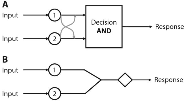
Schematics of parallel interactive channel (A) and coactive processing (B) architectures. note that the coactive architecture pools both sources of information into a single channel.

There are two major types of nonselective influences across channels. One is called indirect nonselective influence (e.g., Townsend, 1984; Townsend & Thomas, 1994), since it arises due to stochastic dependencies (e.g., positive correlations) among the channels. For instance, suppose that Channel 2 feeds all or part of its output into some location on Channel 1 and vice versa. Then the factor that directly affects Channel 2, say X₂, will indirectly affect Channel 1: If an increase in X₂ speeds up activation in Channel 2, it will indirectly also do so in Channel 1.

An extreme version of indirect nonselective influence is found when both channels feed into a final channel where the overall pooled activation can be compared with a single decision criterion. Note that separate channel detections can no longer occur in such a model. This is the kind of model we previewed earlier, known as coactive parallel processing (Figure 4B). The term coactive was first used qualitatively by Miller (1982) to capture “better-than-ordinary-parallel” perceptual data and was later used as a name for mathematical instantiations of the above pooling-into-a-single-channel type of model. A parallel model with (or without) channel interactions but with detections made in each channel (i.e., not coactive) can be called a separate decisions parallel model.

Another type of factor contamination can occur via so-called direct nonselective influence (e.g., Townsend & Thomas, 1994). The name comes from the fact that here, the experimental factors act directly on the separate channels. Hence, instead of, say, activation on Channel 1 being a function of activation on Channel 2 and, therefore, indirectly a function of X₂, a parameter governing the rate of activation on Channel 1 may itself also be a function of a parameter associated with Channel 2.

We have shown that both direct and indirect nonselective influence parallel models can predict positive MIC functions and the proper S-shaped SIC functions. For instance, Townsend and Nozawa (1995) demonstrated that coactive parallel models based on Poisson processes (thus, each Poisson channel feeds its output into a common final channel) inevitably predict a small negative blip, followed by a large positive section of the SIC curve. Fifić (2006) investigated a parallel direct nonselective influence model. It was assumed that each channel possessed a rate that was the product of its “original” rate times the rate of the other channel.

Subsequently, we have been exploring other (indirect nonselective influence) interactive parallel models based on mutual channel facilitation. The full, sophisticated version of mutual facilitation models is based on the parallel Poisson counters of Townsend and Ashby (1983; see also Smith & Van Zandt, 2000). In fact, the independent version of the model is basically identical to the earlier specification. In order to produce positive interactions, it is supposed that some of the counts on one channel can be shared with the other channel with some probability. A full exposition of such models will appear elsewhere. For present purposes, we outline the discrete-time analogue of those models, which can be understood intuitively and which predicts the same qualitative results.

Consider first two parallel and independent channels, with no cross-channel interaction (hence, q = 0). Suppose that a count can occur on each channel with some probability—say, p = .5. The system starts with zero counts, so the initial state of the channels is [0, 0]. Suppose that on the first step, a count occurs on each of the channels, so that the updated state after one step is [1, 1]. Then, on the second iteration, a count occurs on the first channel but not on the second, so the state is [2, 1], and so forth. When both values reach the criterion c, processing terminates. The overall processing time for this simulated trial is then given by the total number of iterations (times a fixed constant that stands for the duration of each iteration).

To model the cross-channel interaction, we allowed each channel to add, on each step, its count to the other channel with a probability of q. So, in the facilitatory model, whenever a count occurs on one of the channels, it is also sent to the other channel with probability q. Consider, then, a facilitatory model in which the probability of cross-channel interaction is q = 1. Then, each count on a given channel is also sent to the other channel. We start again with [0, 0]. On the first step, a count occurs on each of the channels and, at the same time, is sent to the opposite channel, so the system's state after one step is [2, 2]. On the second step, a count occurred on the first channel but not on the second. Nonetheless, due to the interaction, the same count is also sent from the first to the second channel, so that the updated state is [3, 3], and so forth. Note that in this extreme case, in which q = 1, the channels are perfectly correlated and will terminate processing at the same time. Such a model is mathematically equivalent to coactive processing. When q < 1, the channel counts are positively, but partially, correlated.

To model factorial influences, the probability of accumulating a count on the H condition was set to be higher than the probability of a count on the L condition, so that highly salient stimuli resulted in a higher rate of evidence accumulation and, consequently, shorter processing times. The present simulations are based on 1,100 trials per point. A single trial consists of several iterations. Each iteration represents a fixed time interval during which a single unit of evidence (count) can be accumulated with probability p (in a Bernoulli trial). The simulation iterates until the number of counts on each of the channels reaches the prescribed criterion. The processing time represents the total number of iterations.

The critical results of the models' simulations are illustrated in Figure 5. Survivor interaction contrasts for the positively interactive model, for different degrees of interaction, are presented in a sequence of three panels. The leftmost panel corresponds to a zero interaction case (thus, it is really a parallel independent model). Clearly there, SIC(t) is negative at all times, as is predicted by such models (e.g., Townsend & Nozawa, 1995). As we gradually increase the magnitude of the cross-channel interaction (moving on this figure from left to right), the positive part becomes proportionally larger until it exceeds the size of the negative part (resulting, of course, in positive MIC values), just as in much of our data.

Figure 5.

Simulation results of a parallel facilitatory model. The survivor interaction contrast function, SIC(t), starts negative when interaction is set to zero (leftmost panel) and then gradually turns positive as we increase the degree of cross-channel interaction (moving from left to right), until the positive area exceeds the area of the negative part (rightmost panel).

In conclusion, we found S-shaped SIC functions over a wide set of conditions when target–distractor similarity was used as an experimental factor. A number of models were falsified on the basis of major departures from the data. Finally, a promising class of parallel models that assume either positive channel interactions or coactive pooling of activation predict the main qualitative features of the data. Such interactions may be plausible in the context of linguistic-like stimulus patterns, as has been suggested for other configural objects (e.g., Wenger & Townsend, 2001). Naturally, we must finish with the standard caveat that considerably more work will be required to put this inference to the test.

APPENDIX A

In the present study, the stimuli were Cyrillic letter strings. We manipulated the visual dissimilarity between target and test items (and between one test item and others) by constructing them from letters that were drawn either from the same set or from different sets. Target and test items that comprised letters drawn from the same set (say, only curved or only straight-line letters) were considered to have a low visual dissimilarity (for example: Б and В or П and Ш for C = 1; БВ and ВЗ or ШП and НП for C = 2; etc.). If, however, the target item was made of, say, curved letters, and the test items were made of straight-line letters (or vice versa), perceptual discrimination became relatively easy, and they were considered to be highly dissimilar to each other (e.g., Б and П or П and З, for C = 1; БВ and НП or ШП and ВЗ for C = 2; etc.).

We conducted an auxiliary experiment aimed at exploring the effects of visual dissimilarity (high or low) on response latencies across different complexity levels and to validate our dissimilarity manipulation. The setup was identical to that in the visual search experiments, except that the task was to determine whether two simultaneously presented letter strings were identical or different from one another (same–different task). As in the visual search task employed in Experiments 1 and 2, we analyzed different responses only. We hypothesized that the response latencies for items with low dissimilarity would be longer than the response latencies for highly dissimilar items.

Five participants, proficient readers of the Cyrillic alphabet, were presented with two letter strings on a trial and were then asked to indicate (quickly and accurately), by pressing one of two predesignated keys, whether those items were identical to each other or not. Their averaged results, for different response only, are presented in the Figure A1.

The results presented in Figure A1 support our hypothesis and confirm our choice of different letter sets (curved-line vs. straight-line letters) as a valid manipulation of item dissimilarity. A 2 (high dissimilarity or low dissimilarity) × 3 (complexity level 1, 2, or 3) repeated measures ANOVA revealed a significant main effect for item dissimilarity: Mean RTs in the low-dissimilarity condition (M = 860 msec, SD = 19 msec) were significantly longer than mean RTs in the high-dissimilarity condition (M = 624 msec, SD = 33 msec) [F(1,8) = 66.32, p < .01]. In fact, this ordering (slower responses on low dissimilarity trials) was observed for each level of item complexity.

To conclude, mean latencies for different responses for stimulus items that were made up of letters from the same letter set (i.e., both items were made of curved letters, or both items were made of straight-line letters) were longer than response latencies on trials on which the stimulus items were made of letters drawn from different sets (i.e., one item from curved letters, the other from straight-line letters). Hence, the low-dissimilarity experimental condition employed stimuli that were more difficult to tell apart and, therefore, were perceptually less dissimilar to each other. Consequently, these results support using the manipulation of letters from the same set versus letters from different sets as a valid manipulation of item dissimilarity.

Figure A1.

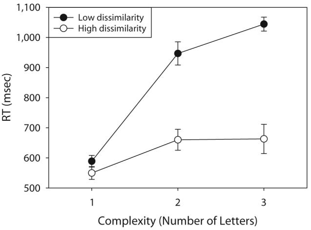
Mean response times (RTs) for responding different to items that shared either low or high visual dissimilarity, as a function of item complexity. The vertical lines represent error bars.

APPENDIX B

In Experiment 1, mean RTs showed a monotonic increase as a function of item complexity. Increasing the complexity of the displayed items by constructing them from more letters resulted in slower responses. In contrast, MIC values did not exhibit a monotonic change, as predicted by simple simulations of known architectures. They increased when moving from the C = 1 to the C = 2 item complexity level but decreased when moving from C = 2 to C = 3, for all participants.

The goal of this analysis is to investigate how mean RTs for each factorial condition (HH, HL, LH, and LL) change across different levels of item complexity. Under the provisional null hypothesis, mean RTs should follow the same trend (say, linear or quadratic) as a function of item complexity for different factorial conditions. In other words, manipulating the complexity level should affect each factorial condition in the same way, given the assumption that the same architecture is engaged in all factorial conditions (HH, HL, LH, and LL).

To test this hypothesis, we conducted a linear regression analysis on mean RTs as a function of item complexity (for the different factorial conditions) for each individual participant, and an additional test with mean RTs averaged over participants. In Figure B1A, we can see that, when averaged across participants, mean RTs in HH and LL conditions increase in a decreasing rate as a function of item complexity, whereas the increase in HL and LH conditions is roughly linear. When a linear regression analysis was performed separately on each individual participant (Figure B1B), a similar pattern was obtained.

Table B1 presents the goodness-of-fit results for the individual analysis, with the averaged r² for different factorial conditions in the bottom row. The proportion of explained variability (r²) is taken as an index of goodness of fit of a linear trend. The two lowest r² scores were obtained for the HH and LL conditions, suggesting, again, that the increase in mean RTs as a function of complexity was less linear on those trials than it was on HL and LH trials.

In our experiments, HH and LL displays differed from HL and LH trials in the mutual similarity between test items: HH displays (alternatively, LL) consisted of two items that were highly similar to each other, whereas the two items presented on HL (LH) trials were dissimilar to each other. Our results and analyses therefore suggest that the mutual similarity between the two test items may interact with the complexity of the items and that this interaction may, in turn, account for the nonmonotonic pattern observed in the MIC values as a function of item complexity. The mechanism underlying this interaction is yet unclear.

Table B1.

A Linear Regression Analysis of Mean Response Times As a Function of Item Complexity (C = 1, 2, or 3) for Different Factorial Conditions (HH, LH, HL, and LL) in Experiment 1

	Factorial Condition
Participant	LL	LH	HL	HH
1	.94	1.00	.99	.73
2	.99	.99	.99	.56
3	.99	.97	.96	.64
4	.98	1.00	1.00	.52
Average	.98	.99	0.98	.61

Note—Goodness-of-fit (r²) values are presented for each individual participant and averaged across participants (bottom row). H, high dissimilarity; L, low dissimilarity.

Figure B1.

A linear regression on mean response times (RTs, in milliseconds) as a function of the item complexity (C = 1, 2, or 3) for different factorial conditions (LL, LH, HH, and HH), in Experiment 1. Panel A presents averaged data (across all 4 participants), and panel B presents the individual data. Goodness-of-fit results (r²) for the averaged data are presented on the right side of panel A; the individual results are presented separately in Table B1. Error bars indicate standard mean errors.

APPENDIX C

Cousineau and Shiffrin (2004) reported that on very difficult target-absent trials, participants did not exhaustively search a displayed set of items. We explored this proposal by simulating both serial and parallel exhaustive architectures, in which the processing of the second item can prematurely stop and, consequently, lead to pure guessing of whether that item is identical to a target item or not. In both architectures, the components are represented in terms of random walk processes that give rise to errors. The simulation results are reported in Table C1. As can be observed, the MIC sign did not show any change to overadditivity for both architectures, although the probability of an error due to the premature completion of the second item increased to 15% for all the factorial conditions. In fact, MIC remained additive for the serial exhaustive model and underadditive for the parallel exhaustive model, thus indicating no change of the sign of the predicted MIC value for both models. We conclude that the overadditivity observed in the L = 2, 3 conditions cannot be accounted for by the premature termination of exhaustive processing.

Table C1.

Simulated Mean Interaction Contrast (MIC) Values for Serial and Parallel Exhaustive Models (50,000 Trials per Condition) for Cases in Which the Error Rate Increases Due to a Premature Termination of Exhaustive Processing of the Second Item

Stimulus Type
HH		HL		LH		LL
RT	p(E)	RT	p(E)	RT	p(E)	RT	p(E)	MIC
Serial Exhaustive
663	.00	906	.00	906	.00	1,149	.00	1
653	.05	884	.05	895	.05	1,127	.05	1
643	.10	858	.10	886	.10	1,101	.10	1
630	.15	829	.15	874	.15	1,073	.15	0
Parallel Exhaustive
647	.00	925	.00	923	.00	1,016	.00	−185
646	.05	909	.05	922	.05	1,011	.05	−174
645	.10	891	.10	923	.10	1,007	.10	−163
644	.15	872	.15	924	.15	1,000	.15	−152

Note—RT, mean response time (in milliseconds); p(E), proportion of errors due to premature termination of exhaustive processing; H, high dissimilarity; L, low dissimilarity.

REFERENCES

- Ashby FG, Townsend JT. Decomposing the reaction time distribution: Pure insertion and selective influence revisited. Journal of Mathematical Psychology. 1980;21:93–123. [Google Scholar]
- Ashby FG, Townsend JT. Varieties of perceptual independence. Psychological Review. 1986;93:154–179. [PubMed] [Google Scholar]
- Atkinson RC, Holmgren JE, Juola JF. Processing time as influenced by the number of elements in a visual display. Perception & Psychophysics. 1969;6:321–326. [Google Scholar]
- Bacon WF, Egeth HE. Overriding stimulus-driven attentional capture. Perception & Psychophysics. 1994;55:485–496. doi: 10.3758/bf03205306. [DOI] [PubMed] [Google Scholar]
- Bundesen C. A theory of visual attention. Psychological Review. 1990;97:523–547. doi: 10.1037/0033-295x.97.4.523. [DOI] [PubMed] [Google Scholar]
- Colonius H, Townsend JT. Activation-state representation of models for the redundant-signals-effect. In: Marley AAJ, editor. Choice, decision, and measurement. Erlbaum; Mahwah, NJ: 1997. pp. 245–254. [Google Scholar]
- Cousineau D, Shiffrin RM. Termination of a visual search with large display size effects. Spatial Vision. 2004;17:327–352. doi: 10.1163/1568568041920104. [DOI] [PubMed] [Google Scholar]
- Diederich A, Colonius H. A further test of the superposition model for the redundant-signals effect in biomodal detection. Perception & Psychophysics. 1991;50:83–86. doi: 10.3758/bf03212207. [DOI] [PubMed] [Google Scholar]
- Duncan J, Humphreys GW. Visual search and stimulus similarity. Psychological Review. 1989;96:433–458. doi: 10.1037/0033-295x.96.3.433. [DOI] [PubMed] [Google Scholar]
- Dzhafarov EN. Process representations and decompositions of response times. In: Marley AAJ, editor. Choice, decision, and measurement. Erlbaum; Mahwah, NJ: 1997. pp. 255–278. [Google Scholar]
- Dzhafarov EN. Conditionally selective dependence of random variables on external factors. Journal of Mathematical Psychology. 1999;43:123–157. doi: 10.1006/jmps.1998.1231. [DOI] [PubMed] [Google Scholar]
- Egeth HE. Parallel versus serial processes in multidimensional stimulus discrimination. Perception & Psychophysics. 1966;1:245–252. [Google Scholar]
- Egeth HE, Dagenbach D. Parallel versus serial processing in visual search: Further evidence from subadditive effects of a visual quality. Journal of Experimental Psychology: Human Perception & Performance. 1991;17:550–559. doi: 10.1037//0096-1523.17.2.551. [DOI] [PubMed] [Google Scholar]
- Fifić M. Emerging holistic properties at face value: Assessing characteristics of face perception. Indiana University; Bloomington: 2006. Unpublished doctoral dissertation. [Google Scholar]
- Folk CL, Remington R. Selectivity in distraction by irrelevant featural singletons: Evidence for two forms of attentional capture. Journal of Experimental Psychology: Human Perception & Performance. 1998;24:847–858. doi: 10.1037//0096-1523.24.3.847. [DOI] [PubMed] [Google Scholar]
- Grossberg S, Mingolla E, Ross WD. A neural theory of attentive visual search: Interactions of boundary, surface, spatial, and object representations. Psychological Review. 1994;101:470–489. doi: 10.1037/0033-295x.101.3.470. [DOI] [PubMed] [Google Scholar]
- Hughes HC, Townsend JT. Varieties of binocular interaction in human vision. Psychological Science. 1998;9:53–60. [Google Scholar]
- Innes-Ker AHK. Gestalt perception of emotional expressions. Indiana University; Bloomington: 2003. Unpublished doctoral dissertation. [Google Scholar]
- McElree B, Carrasco M. The temporal dynamics of visual search: Evidence for parallel processing in feature and conjunction searches. Journal of Experimental Psychology: Human Perception & Performance. 1999;25:1517–1539. doi: 10.1037//0096-1523.25.6.1517. [DOI] [PMC free article] [PubMed] [Google Scholar]
- Miller J. Divided attention: Evidence for coactivation with redundant signals. Cognitive Psychology. 1982;14:247–279. doi: 10.1016/0010-0285(82)90010-x. [DOI] [PubMed] [Google Scholar]
- Mordkoff JT, Yantis S. An interactive race model of divided attention. Journal of Experimental Psychology: Human Perception & Perfomance. 1991;17:520–538. doi: 10.1037//0096-1523.17.2.520. [DOI] [PubMed] [Google Scholar]
- Palmer J, Verghese P, Pavel M. The psychophysics of visual search. Vision Research. 2000;40:1227–1268. doi: 10.1016/s0042-6989(99)00244-8. [DOI] [PubMed] [Google Scholar]
- Pashler H, Harris CR. Spontaneous allocation of visual attention: Dominant role of uniqueness. Psychonomic Bulletin & Review. 2001;8:747–752. doi: 10.3758/bf03196213. [DOI] [PubMed] [Google Scholar]
- Sagi D, Julesz B. “Where” and “what” in vision. Science. 1985;228:1217–1219. doi: 10.1126/science.4001937. [DOI] [PubMed] [Google Scholar]
- Schweickert R. A critical path generalization of the additive factor method: Analysis of a Stroop task. Journal of Mathematical Psychology. 1978;18:105–139. [Google Scholar]
- Schweickert R, Giorgini M, Dzhafarov E. Selective influence and response time cumulative distribution functions in serial–parallel task networks. Journal of Mathematical Psychology. 2000;44:504–535. doi: 10.1006/jmps.1999.1268. [DOI] [PubMed] [Google Scholar]
- Schweickert R, Townsend JT. A trichotomy: Interactions of factors prolonging sequential and concurrent mental processes in stochastic discrete mental (PERT) networks. Journal of Mathematical Psychology. 1989;33:328–347. [Google Scholar]
- Smith PL, Van Zandt T. Time-dependent Poisson counter models of response latency in simple judgment. British Journal of Mathematical & Statistical Psychology. 2000;53:293–315. doi: 10.1348/000711000159349. [DOI] [PubMed] [Google Scholar]
- Sternberg S. High-speed scanning in human memory. Science. 1966;153:652–654. doi: 10.1126/science.153.3736.652. [DOI] [PubMed] [Google Scholar]
- Sternberg S. The discovery of processing stages: Extensions of Donders' method. Acta Psychologica. 1969;30:276–315. [Google Scholar]
- Thornton TL, Gilden DL. Parallel and serial processes in visual search. Psychological Review. 2007;114:71–103. doi: 10.1037/0033-295X.114.1.71. [DOI] [PubMed] [Google Scholar]
- Townsend JT. Proceedings of the Purdue Centennial Symposium on Information Processing. Purdue University Press; West Lafayette, IN: 1969. Mock parallel and serial models and experimental detection of these; pp. 617–628. [Google Scholar]
- Townsend JT. A note on the identifiability of parallel and serial processes. Perception & Psychophysics. 1971;10:161–163. [Google Scholar]
- Townsend JT. Some results concerning the identifiability of parallel and serial processes. British Journal of Mathematical & Statistical Psychology. 1972;25:168–199. [Google Scholar]
- Townsend JT. Uncovering mental processes with factorial experiments. Journal of Mathematical Psychology. 1984;28:363–400. [Google Scholar]
- Townsend JT. Truth and consequences of ordinal differences in statistical distributions: Toward a theory of hierarchical inference. Psychological Bulletin. 1990;108:551–567. doi: 10.1037/0033-2909.108.3.551. [DOI] [PubMed] [Google Scholar]
- Townsend JT, Ashby FG. Methods of modeling capacity in simple processing systems. In: Castellan J, Restle F, editors. Cognitive theory. III. Erlbaum; Hillsdale, NJ: 1978. pp. 200–239. [Google Scholar]
- Townsend JT, Ashby FG. The stochastic modeling of elementary psychological processes. Cambridge University Press; Cambridge: 1983. [Google Scholar]
- Townsend JT, Fifić M. Parallel versus serial processing and individual differences in high-speed search in human memory. Perception & Psychophysics. 2004;66:953–962. doi: 10.3758/bf03194987. [DOI] [PubMed] [Google Scholar]
- Townsend JT, Nozawa G. Strong evidence for parallel processing with simple dot stimuli; Paper presented at the 29th Annual Meeting of the Psychonomic Society; Chicago. Nov, 1988. [Google Scholar]
- Townsend JT, Nozawa G. Spatiotemporal properties of elementary perception: An investigation of parallel, serial, and coactive theories. Journal of Mathematical Psychology. 1995;39:321–359. [Google Scholar]
- Townsend JT, Roos RN. Search reaction time for single targets in multiletter stimuli with brief visual displays. Memory & Cognition. 1973;1:319–332. doi: 10.3758/BF03198116. [DOI] [PubMed] [Google Scholar]
- Townsend JT, Thomas RD. Stochastic dependencies in parallel and serial models: Effects on systems factorial interactions. Journal of Mathematical Psychology. 1994;38:1–34. [Google Scholar]
- Townsend JT, Wenger MJ. The serial–parallel dilemma: A case study in a linkage of theory and method. Psychonomic Bulletin & Review. 2004a;11:391–418. doi: 10.3758/bf03196588. [DOI] [PubMed] [Google Scholar]
- Townsend JT, Wenger MJ. A theory of interactive parallel processing: New capacity measures and predictions for a response time inequality series. Psychological Review. 2004b;111:1003–1035. doi: 10.1037/0033-295X.111.4.1003. [DOI] [PubMed] [Google Scholar]
- Treisman A, Gelade G. A feature-integration theory of attention. Cognitive Psychology. 1980;12:97–136. doi: 10.1016/0010-0285(80)90005-5. [DOI] [PubMed] [Google Scholar]
- Treisman A, Sato S. Conjunction search revised. Journal of Experimental Psychology: Human Perception & Performance. 1990;16:459–478. doi: 10.1037//0096-1523.16.3.459. [DOI] [PubMed] [Google Scholar]
- Wenger MJ, Townsend JT. Faces as gestalt stimuli: Process characteristics. In: Wenger MJ, Townsend JT, editors. Computational, geometric, and process perspectives on facial cognition: Contexts and challenges. Erlbaum; Mahwah, NJ: 2001. pp. 229–284. [Google Scholar]
- Wenger MJ, Townsend JT. On the costs and benefits of faces and words: Process characteristics of feature search in highly meaningful stimuli. Journal of Experimental Psychology: Human Perception & Performance. 2006;32:755–779. doi: 10.1037/0096-1523.32.3.755. [DOI] [PubMed] [Google Scholar]
- Wolfe JM. Guided Search 2.0: A revised model of visual search. Psychonomic Bulletin & Review. 1994;1:202–238. doi: 10.3758/BF03200774. [DOI] [PubMed] [Google Scholar]
- Wolfe JM. What can 1 million trials tell us about visual search? Psychological Science. 1998;9:33–39. [Google Scholar]
- Wolfe JM, Cave KR, Franzel SL. Guided search: An alternative to the modified feature integration model for visual search. Journal of Experimental Psychology: Human Perception & Performance. 1989;15:419–433. doi: 10.1037//0096-1523.15.3.419. [DOI] [PubMed] [Google Scholar]
- Zelinsky GJ, Sheinberg DL. Eye movements during parallel–serial visual search. Journal of Experimental Psychology: Human Perception & Performance. 1997;23:244–262. doi: 10.1037//0096-1523.23.1.244. [DOI] [PubMed] [Google Scholar]