Ultra High Resolution ¹H-¹³C HSQC Spectra of Metabolite Mixtures using non-linear sampling and Forward Maximum Entropy (FM) Reconstruction

Abstract

To obtain a comprehensive assessment of metabolite levels from extracts of leukocytes, we have recorded ultra-high-resolution ¹H-¹³C HSQC NMR spectra of cell extracts, which exhibit spectral signatures of numerous small molecules. However, conventional acquisition of such spectra is time consuming and hampers measurements on multiple samples, which would be needed for statistical analysis of metabolite concentrations. Here we show that the measurement time can be dramatically reduced without loss of spectral quality when using non-linear sampling (NLS) and a new high-fidelity Forward Maximum-entropy (FM) reconstruction algorithm. This FM reconstruction conserves all measured time domain data points and guesses the missing data points by an iterative process. This consists of discrete Fourier transformation of the sparse time-domain data set, computation of the spectral entropy, determination of a multidimensional entropy gradient, and calculation of new values for the missing time domain data points with a conjugate gradient approach. Since this procedure does not alter measured data points it reproduces signal intensities with high fidelity and does not suffer from a dynamic-range problem. As an example we measured a natural abundance ¹H-¹³C HSQC spectrum of metabolites from granulocyte cell extracts. We show that a high-resolution ¹H-¹³C HSQC spectrum with 4k complex increments recorded linearly within 3.7 days can be reconstructed from 1/7^th of the increments with nearly identical spectral appearance, indistinguishable signal intensities and comparable or even lower root mean square (rms) and peak noise patterns measured in signal-free areas. Thus, this approach allows recording of ultra-high resolution ¹H-¹³C HSQC spectra in a fraction of the time needed for recording linearly sampled spectra.

Introduction

Comprehensive measurements of the concentrations of large numbers of metabolites can provide detailed insights into the state of cells ^{1, 2}. This has the potential of being used to diagnose disease, to follow the effect of drug treatment, or to study toxicity. Comparison of metabolite samples from different groups, such as healthy and sick individuals, or normal and transformed cells may lead to identification of biomarkers that can be invaluable for targeted disease diagnosis or for understanding metabolic pathways and mechanisms of disease. Metabolic profiling of cell lines may lead to new insights into metabolic pathways and their alteration in disease.

Assessment of metabolite levels in metabolomics studies has primarily relied on mass spectroscopy, NMR spectroscopy, chromatographic separation techniques and various multivariate data analysis techniques ^1-3. Among the NMR methods, one dimensional (1D) ¹H spectroscopy is most commonly used, where the spectrum is divided in a limited number of buckets. These signal intensities of the buckets are either directly compared between multiple samples using principle component analysis (PCA), or, if a prior model is assumed, partial least square discriminant analysis (PLS-DA) or similar statistical approaches are used in order to separate groups of samples. All of this in an effort to identify the metabolites (biomarkers) that are most different between the groups ⁴. Alternatively, 1D NMR spectra have been directly fitted to databases of metabolite reference spectra to obtain concentrations of the most abundant molecules in a metabolite mixture ⁵. Occasionally, two-dimensional NMR spectra have been used to enhance the spectroscopic resolution for more detailed metabolite identification ^6-10. Resonances of metabolites typically have very long transverse relaxation times so that 2D NMR spectra, such as ¹H-¹³C HSQC or ¹H-¹H TOCSY, can principally be recorded at very high resolution and can resolve nearly all metabolite signals. However, this requires a large number of increments, which makes data acquisition very time consuming and impractical for recording spectra from multiple samples as is necessary for statistical analysis.

It has been proposed and experimentally verified in the past that the measuring times of 2D NMR spectra can be reduced with non-linear sampling in the indirect dimensions ^{11, 12}. Barna and coworkers sampled 2D NMR data with an exponential schedule ¹³ and processed the data with a maximum entropy method (MEM) relying on the Burg algorithm ¹⁴. Subsequently, non-linear sampling was seriously pursued by several other groups ^{15 16-18 19}. Processing software was developed that relied on an alternative maximum entropy (MaxEnt) reconstruction algorithm that could handle phase-sensitive data and included adjustable parameters to tune the outcome of the data reconstruction. This software is available through the Rowland NMR Toolkit (RNMRTK) ¹⁵ and has been successfully applied for processing 2D non-linearly sampled COSY spectra ²⁰, constant-time evolution periods of triple-resonance data ²¹, or quantification of HSQC spectra for relaxation experiments ²². Development of a two-dimensional MaxEnt reconstruction procedure designed to run in parallel on workstation clusters ²³ has stimulated several applications to explore optimum evolution times ²⁴, to rapidly acquire complete sets of triple resonance experiments for sequential assignments ²⁵, to facilitate side-chain assignments ²⁶, and to enable high-resolution triple resonance experiments ^{27, 28}.

The principle advantages of non-linear sampling are increasingly recognized ²⁹. Besides Maximum Entropy reconstruction, other methods are used for processing non-linearly recorded spectra, such as the maximum likelyhood method (MLM) ³⁰, a Fourier transformation of nonlinearly spaced data using the Dutt-Rokhlin algorithm ³¹, or multi-dimensional decomposition (MDD) ^32-35.

A special case for reducing the time to record 3D or higher-dimensional data is used with sampling along various angles of the indirect sampling space ^{36, 37}, and previously developed projection-reconstruction procedures ³⁸ are used for processing the data. Another strategy for minimizing sampling times is the reduced dimensionality approach ³⁹, which has been further developed into the GFT method ⁴⁰ and applied to proteins up to 21 kDa ⁴¹. However, to our knowledge, the projection reconstruction method and the GFT approach have primarily been applied to rather small systems where sensitivity is less of an issue. Unlike MaxEnt reconstruction, this class of approaches is only suited for 3D and higher dimensional experiments but not applicable to shortening acquisition of 2D experiments.

In the past, we have used the MaxEnt reconstruction procedure of the Rowland NMR Toolkit (RNMRTK) ¹². It is very efficient and ideally suited for handling non-linearly sampled data with a low dynamic range, such as triple-resonance spectra where all peaks have similar intensities. However, processing of data with a large variation of peak intensities, such as in NOESYs, TOCSYs, mixtures of metabolites, spectra with diagonals or peaks close to the noise level seems to suffer from effects of non-linearity of peak intensities. This has previously been recognized and remedies for correcting intensities have been suggested for MaxEnt reconstructions of relaxation data ⁴². However, there remains the problem of losing weak peaks that are barely above noise level, which is a significant problem in spectra of metabolite mixtures with large variations peak intensities.

As another strategy to cope with the dynamic range problem we will examine whether this issue can be eliminated by using a new maximum-entropy related approach that operates on a different principle. In the classic MaxEnt algorithm, such as used by Hoch and Stern⁴³, the linearity of the reconstruction depends of the parameter λ (lambda), a Lagrange multiplier that is required to create the objective function Q(f) = S(f) - λC(f,d). $S(f)=-\text{∑}_{k=1}^N{f}_{k}log{f}_k$ is the Shannon entropy (which has the same form as Gibbs' entropy, yet applies to information content), and C(f,d) is the constraining function between the measured time domain data points and those calculated from the inverse Fourier transformed iteratively “guessed” mock spectra. By the nature of altering the spectra in the frequency domain, C(f,d) is always > 0, except in very rare cases. In general, keeping it at zero does not allow for alteration of data points in the frequency domain.

Here we present a new procedure termed Forward Maximum entropy (FM) reconstruction for processing non-linearly sampled 2D NMR data. Similarly to the MaxEnt reconstruction of Hoch and Stern ¹², it aims to minimize a target function that contains the negative entropy. However, in contrast to the MaxEnt reconstruction procedure ⁴³, which allows a variation of the measured data points by maximizing the target function Q(f) = S(f) - λC(f,d), the FM reconstruction only optimizes the time domain data points that have not been measured and does not allow for variation of the acquired time-domain data points. We claim that this approach assures high fidelity of peak intensity reconstruction. Thus, all experimental measured data points are strictly conserved, which we claim enforces correct relative intensities. In contrast, a procedure that allows variation of measured data points to minimize the target function Q(f) is tempted to do this on the expense of weak peaks. By altering the method such that the “guessing” occurs in the time domain, the constraining function C(f,d) can easily be set to zero, and the requirement of the Lagrange multiplier thus vanishes. The objective function is now reduced to Q(f) = S(f). The implementation hence requires the “mock” data to be constantly “guessed” in the time domain, then forward Fourier transformed, where they are scored by only calculating the implemented Entropy function. This approach doesn't seriously bias against weak signals. We validate this approach with a ¹H-¹³C HSQC spectrum of metabolites from cell extracts recorded with 8k real increments. Acquisition of the linearly sampled reference spectrum required 3.7 days on a 600 MHz spectrometer. We show that the same quality of spectrum can be obtained within fourteen hours using non-linear sampling and the FM reconstruction. This makes possible recording of multiple ultra high-resolution ¹H-¹³C HSQC spectra needed for statistical analysis of metabolomics data.

Materials and Methods

Principles of the Forward Maximum Entropy (FM) Reconstruction

We pursue to reconstruct a complex time-domain data set F(d) = {d_i; i = 1 ..N} where a subset of points {d_k; k = 1 ..M} (M < N) has been measured experimentally but all other points are unknown. We guess the unknown data points in the time domain. Initially, all unknown points are set to complex zero or 0+i0. Subsequently we process the spectrum with the fast the Fourier transform (FFT) algorithm and calculate its entropy:

$$S(f)=-\sum _{k=1}^N{f}_{k}log{f}_k$$

Because many of the data points are fixed and given by the experimental data set d, we may use a simplistic approach of the Entropy S(f) for complex data points f_k, namely

$$S(f)=-\sum _{k=1}^N\left|f_k\right|log\left|f_k\right|.$$

We pursue to maximize Q(f) = S(f) iteratively using the Forward Maximum entropy (FM) reconstruction method proposed here that maintains the experimental time domain data points unaltered. Since this approach is equivalent to minimizing the negative entropy we define the target function T(f) = -S(f), which we aim to minimize. T(f) is related to the norm of a spectrum, and minimizing it reduces the total signal and noise subject to maintaining the measured time-domain data points.

The FM reconstruction program described here starts by setting the missing time-domain data points to zero. The data are then transformed with the fast Fourier transform (FFT) algorithm, and the target function of the resulting spectrum is calculated. Next, the guessed time-domain data points are changed by ± δ, followed by FFT and calculation of the target functions. From the resulting values a multidimensional gradient of T(f), $\overrightarrow{\nabla }T(f)$, is calculated with respect to the missing data points d_j. Using this gradient we minimize T(f) with the Polak-Ribiere conjugate gradient method ⁴⁴ to gradually change the guesses of the missing time-domain data points d_j. In the minimization, the real and the imaginary parts of the time domain data points d_j are treated as independent variables. This creates a total of 2 * (N − M) free vectors of $\overrightarrow{\nabla }T(f)$, where N is the number of grid (final) points, and M is the number of measured time points (see above), and the difference of N and M is multiplied by two, because each point is of complex nature, and the real and imaginary components are minimized independently of each other. For initialization purpose, all missing data points are set to zero.

Minimization is iterated until a cut-off criterion is reached, such as that the value of the target function T(f) does not decrease by more than the cut-off parameter, the gradient $\overrightarrow{\nabla }T(f)$ is sufficiently small, or a maximum number of desired iterations have been reached.

The final result of the FM reconstruction procedure is a time-domain data set where the missing data points are filled in with the optimum values obtained by minimizing T_F. This time-domain data set can now be transformed with any available data processing software and can be manipulated with window functions, zero filling and/or linear prediction.

Practical implementation of FM reconstruction

The package FFTW (http://www.fftw.org), version 3.0.1 was used as a C library for computing discrete Fourier transforms. FFTW is distributed under the GNU software licenses and is free software. The Polak-Ribiere conjugate gradient method, gsl_multimin_fdsminimizer_conjugate_pr of the package GSL, vers 1.5 (GNU Scientific Library, http://www.gnu.org/software/gsl), was used for minimization purposes. For data handling, we used the open NMRPipe data format for describing NMR data. See http://spin.niddk.nih.gov/bax/softgware/NMRPipe for a description of NMRPipe. The resulting C program was initially compiled using gcc and the i686 instruction set on a Dell dual Xenon 3.0 GHz computer operating under Fedora Core 1 Linux OS. The program has since been compiled and run on other RedHat Linux computers. This includes use of 64-bit Opteron computers. The program will be made available on demand through our website at http://gwagner.med.harvard.edu.

Generation of sampling schedules

Three different sampling schedules, S1, S2 and S3 were used to pick increments from the total data set. For S1, increments were picked randomly but with constant density along t₁. S2 and S3 also sample randomly but the sampling density is not constant. S2 used an exponentially decreasing sampling density, and S3 applied a linearly decreasing pick rate. The random sampling schedules are created based on Unix tools with the following procedure: First, a vector is created with the length of the final number of complex slots N (4096 in our case) with associated ordinal number, starting at 0. Second, in each slot, a number is placed that represents the sampling density. For the constant density of schedule S1 this is 1.0 for each slot. For the exponentially decaying density of schedule S2 this is 1.0 for slot 0 and exp{-i/(N-1)} for slot i =1 to N-1. For the linear ramp of schedule S3 this is 1.0 for slot 0 and 1.0-i/N for slot i= 1 to N-1. Third, the sum SU(Sk) of all slot values is calculated for each of the schedules Sk (S1, S2, S3). Fourth, a random number is generated with the function drand48, which yields a 48 bit random number in the range from 0.0 trough 1.0. This random value is multiplied by the sum SU(Sk) for each of the three schedules. Fifth, the values in the respective slots are cumulatively added to the point where the sum is larger than the value created in point #4 above. Sixth, the slot number is now registered as a point to be sampled in the non-linear acquisition, and the slot value is now set to zero, which reduces the value of the sum SU(Sk) for the next round. Seventh, the points, #3, 4, 5 and 6 are repeated until the desired number of sampling points of the non linear sampling schedule is reached, and the numbers are then sorted.

To initialize the random function drand48, a seed number is required. Either, a rationally chosen seed number may be given, or a seed number can be created from the internal clock which registers number of seconds since New Years Day, 1970, 0.00.00. The latter is the reference point for UNIX. While both approaches yield good results, we have noticed that certain seed numbers yield slightly better reconstructions and speedier convergence than others. Thus, choosing “favorite” or “rationally chosen” seed numbers may be preferable to optimize the obtainable results. For further information on selecting random numbers, and the use of drand48, we refer to the UNIX manuals.

Preparation of cell extracts from mouse Baf3 cells

Mouse BaF3 cells were obtained from Dr. James Griffin at the Dana Farber Cancer Institute. BaF3 is a murine blood cell line dependent of IL-3 for survival and differentiation. Cells were cultured in the presence of 5% CO₂ at 37°C in RPMI 1640 medium supplemented with 10% fetal calf serum, and penicillin/streptomycin. Media for BaF3 was additionally supplemented with WEHI 3B conditioned medium as a source of IL-3. About 2 billion cells (ca. 3 ml) were lysed by the sequential addition of 4 ml of methanol, 4 ml of chloroform and 4 ml of water. The sample was vortexed vigorously after the addition of each solvent and the final mixture was stored at −20 °C overnight for phase separation. Complete separation of phases was achieved by centrifugation at 10,000 × g for 40 minutes. Only the aqueous phase was used here. It was lyophilized and dissolved in ²H₂O for the NMR experiments. Extracts from 2 × 10⁹ cells were used for the sample.

NMR spectroscopy

NMR spectra were recorded on a Bruker Avance 600 spectrometer equipped with a cryogenic triple-resonance probe. A set of seven ¹H-¹³C HSQC spectra were recorded with 4k increments (complex) and 4 scans per increment. A relaxation delay of 1.2 seconds was used between scans. Each of the seven spectra was recorded in 12.7 hours; the total measurement time for all seven 2D spectra was 3.7 days.

Results

Recording an ultra high resolution (UHR) ¹H-¹³C HSQC spectrum

As a first step towards identifying metabolites in BaF3 cells we have recorded a 1D spectrum of the aqueous phase of cell extracts in ²H₂O, which is shown in Fig. 1A. Identification and measurement of concentrations of metabolites is severely hampered by spectral overlap. Similarly, 2D NMR spectra recorded with the typically 100 to 200 increments suffer from low resolution in the indirect dimension. Thus, we recorded, an ultra high resolution (UHR) ¹H-¹³C HSQC spectrum with 4k increments (complex data points) (Figure 1B). The signal separation obtained with 4k complex increments resolves essentially all overlap as is shown with the expansion of the most crowded region in Fig. 1D. The dispersion of the UHR spectrum promises to provide a tool for assigning nearly all metabolites that are present in sufficiently high concentrations and for measuring concentrations of the individual metabolites.

Figure 1.

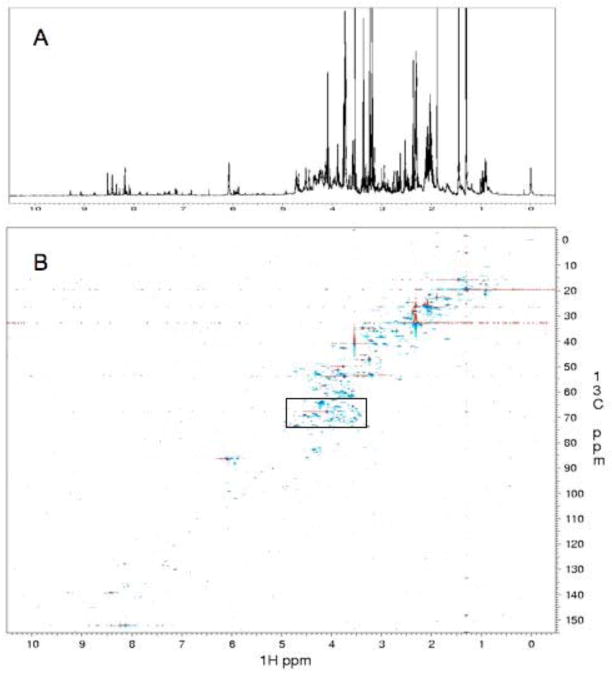
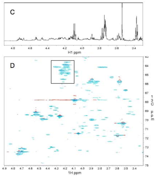
NMR spectra of the aqueous fraction of cell extracts from mouse BaF3 cells in ²H₂O, pH 6.5, 25° C. A. One-dimensional ¹H NMR spectrum. B. ¹H-¹³C HSQC spectrum recorded with 4k complex points in the indirect dimension. C and D. Expansion of the section indicated with the box in B and corresponding 1D spectrum. Note that the 2D spectrum of Fig. 1C is a small portion of the entire spectrum. The 1D spectrum of Figure 1C contains also signals from outside the ¹³C region of Fig. 2D (compare Fig. 1A and 1B).

The 4k complex increments result in a maximum t₁ value of 0.16 sec. This is rather long compared to typically recorded 2D ¹H-¹³C HSQC experiments; however, it should be compared with the transverse relaxation times for metabolite carbons, which are in the order of one or several seconds. As stated previously, it is desirable to sample evolution times close to T₂ to obtain optimal resolution and sensitivity ²⁴, which is still far off with the conditions used here. To experimentally examine the optimal number of increments for the sample used here, we transformed the data set using 4k, 2k, 1k and 512 complex t₁ values. Figure 2 shows the effect on a small crowded region that is indicated with a box in Fig. 1D. To have comparable scaling all data sets were multiplied with a cosine window and zero-filled to 8k points. This ensures identical scaling with the number of points in the FIDs. The 4k and 2k data clearly resolve all peaks but the transformations of only 1024 and 512 increments do not. A cross section drawn through the strongest peak demonstrates that increased resolution also results in larger peak height. Thus, the relative height of the tallest peak is 3.9 : 3.0 : 2.0 : 1.0 in the 4k, 2k, 1k and 512 point transforms, respectively (Fig. 2). Although the apparent resolution doesn't improve much by going from 2k to 4k complex data points in t₁ the peak height increases by approximately 30%, which is close to $\sqrt{2}$ (41% increase) and consistent with the expectation (Fig. 2). Obviously, doubling the number of t₁ values from 2k to 4k doubles the measuring time, and the spectrum shown here required a total of 3.7 days of instrument time. This is undesirably long if one wants to measure multiple samples for determining statistically significant differences of metabolite concentrations between cell types or different populations of the same cells. It is indeed the long-term goal of our research to identify metabolites with concentrations that differ between cell samples. This includes comparison of normal and malignant cells, cells before and after treatment with drugs, or any other pairs of distinct cell types. Measurement of multiple samples for each cell samples would be difficult with measurement times of 3.7 days as was used for the spectrum in Fig.1.

Figure 2.

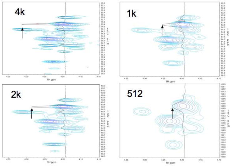
Comparison of a small spectral region indicated with a box in Fig. 1D transformed with different numbers of increments. Clearly, only 2k and 4k complex points can resolve all peaks. While 2k complex increments seem to resolve all peaks, going to 4k complex points sharpens the peaks and increases the peak height by approximately 30% (see arrows). To obtain equal scaling in all four cases, the measured data points were multiplied with a cosine bell and zero-filled to 8k real points.

To reduce the measurement time we have explored the non-linear sampling approach with the Forward Maximum Entropy (FM) reconstruction for data processing. We hypothesized that this approach allows recording of high-resolution 2D spectra within a reasonably short time, and developed the FM with the goal to avoid bias against weak peaks.

To test this approach we have recorded seven identical linearly sampled high resolution ¹H-¹³C HSQC spectra acquired over a period of 12.7 hours each. Addition of the seven spectra and standard FFT yields the spectrum shown in Fig. 1. Recording all seven spectra required 3.7 days of instrument time. The high resolution achieved is demonstrated by showing an expansion of a small portion of the most crowded spectral region (Fig. 1C). Numerous ¹H-¹³C cross peaks are visible and all are very well resolved.

Impact of non-linear sampling with FM reconstruction on resolution and S/N

To avoid impractically long measuring times and enable measurements on several samples for statistical analysis, we tested whether non-linear sampling and a suitable processing routine would allow shortening the measurement time. Since spectra of mixtures of metabolites have a large variation of intensities we employed the FM reconstruction approach outlined above. To test this we have recorded the data set described above. To get the sub-sets of non-linearly sampled data we (1) add all seven data sets together, (2) we select a non-linear sampled regime from the combined data set using 1/7th of the increments. This allowed us to compare spectra recorded linearly within 12.7 hrs with data recorded non-linearly within the same amount of time, with only 1/7^th of the increments but seven times the number of scans per increment.

Figure 3 shows different versions of a representative cross section along the carbon dimension of the ¹H-¹³C HSQC spectrum of Figure 1. Figure 3A provides transformations of all linearly acquired data points. The lower three traces are from spectra 2, 4 and 6 out of the seven spectra recorded for 12.7 hrs each, using 16 scans per increment. (Note that the peak at 57.35 ppm decreases with time due to metabolic changes ongoing in the sample; it is only visible in spectra 1 – 3 and disappears in later spectra. Although we tried to stabilize the metabolite samples some peaks change over a period of 3.7 days, and the individual spectra were not entirely identical. It was indeed a motivation for developing the fast method described here to avoid long-term changes in the metabolite samples.) The top spectrum is the sum of all seven spectra and represents a measuring time of 3.7 days with 7 × 16 scans per increment. It demonstrates the gain in signal to noise by a factor of $\sqrt{7}$ compared to the individual spectra, such as 2, 4 or 6 shown in the lower part of the figure. The top spectrum of Fig. 3B is the same as in Fig. 3A. The lower three traces, however, are FM reconstructions using only one 1/7^th of the increments but 7 × 16 scans per increment. Thus each of the lower three traces represents the same total measuring time of 12.7 hours, equal to each of the lower traces of Fig. 3A. Three different sampling schedules, S1, S2 and S3 were used to pick increments from the total data set. For S1, increments were picked randomly but with constant density along t₁. S2 and S3 also sample randomly but the sampling density is not constant. S2 used an exponentially decreasing sampling density, and S3 applied a linearly decreasing pick rate. As can be seen, the quality of the three non-linearly sampled spectra, transformed with FM, is comparable to the top trace, which represents a seven-fold longer measurement time. There is no obvious bias in favor of strong peaks or against weak peaks. The three sampling schedule exhibit similar results but the schedule with exponentially decreasing weight (S2) seems to have the best signal-to-noise ratio with a small margin. A more systematic examination of sampling schedules will be required, however, to optimize this procedure.

Figure 3.

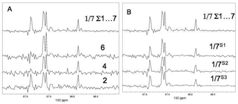
Comparison of representative cross sections along the ¹³C direction at a proton frequency of 3.76 ppm. (A) Use of the full linearly sampled data. The bottom three traces are from the full linearly sampled data sets 2, 4 and 6. The top trace is from the average of all seven linearly sampled data sets (sum of all seven spectra divided by 7). (B) The top trace is the same as in A. The three traces at the bottom, however, are obtained by selecting 1/7^th of the increments of the averaged data set and transformed with FM reconstruction. In the sampling schedule S1 1/7^th of the increments were picked randomly from the averaged data set with equal density along t₁. In schedule S2, 1/7^th of the increments were picked with exponentially decreasing density, and in schedule S3, 1/7^th of the increments were picked with linearly decreasing density. Note that the peak at 57.35 ppm disappears with time and is only visible in spectra 1 – 3. Although we tried to stabilize the metabolite samples some peaks change over a period of 3.7 days. Thus, the spectra 2, 4 and 6 are not entirely identical.

To further assess the quality of the NLS spectra processed with FM reconstruction we analyzed the apparent noise in the linearly and non-linearly sampled spectra. Figure 4 shows a small representative section of the ¹H-¹³C HSQC spectrum that contains strong and weak peaks. And cross sections through the strongest peak along the carbon dimensions were plotted on top of the contour plots. The traces from the linearly sampled spectrum (4 days measuring time) and the non-linearly sampled spectrum (12.7 hrs measuring time) are essentially indistinguishable.

Fig. 4.

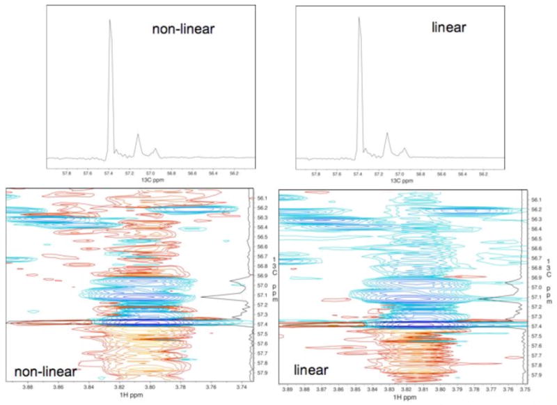
Comparison between the linearly sampled 3.7-day experiment and the NLS/FM reconstruction of a 12.7-hrs subset of increments. Both the 2D plot of a small portion of the spectrum and the cross section along the ¹³C direction at the position of the strongest peak are nearly indistinguishable. This demonstrates the high fidelity of the FM reconstruction.

For further comparison of the quality of the two spectra, the apparent noise was measured in a region outside the range that contains signals (Fig. 5). Both the root mean square (rms) noise and the peak noise were measured for the three linearly sampled spectra 2, 4 and 6, as well as the average of all seven linearly recorded spectra. As expected, both the rms and peak noise are approximately $\sqrt{7}$ lower when averaging the seven linearly sampled spectra (left and middle columns). Importantly, the FM reconstruction of the NLS data picked from the averaged data set have roughly the same peak noise as the full averaged data; it is lowest for the exponential schedule S2. For all three sampling schedules, the rms noise is approximately two-fold lower than in the transform of the full linear averaged data set. Thus, the FM processing of the NLS data sets, which can be acquired in 1/7^th of the measuring time, yield high quality spectra comparable in quality to the DFT of the full linearly sampled averaged data set (Fig. 5, middle and right columns).

Figure 5.

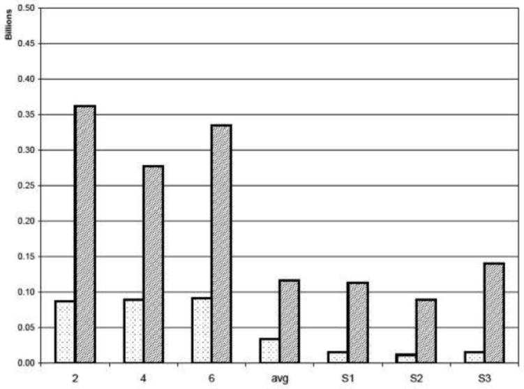
Comparison of rms noise (light) and peak noise (dark) of the cross sections along the ¹³C dimension. Both rms and peak noise are measured outside of the region that contains signals. The columns labeled 2, 4 and 6 represent three of the seven linearly sampled spectra of 12.7 hours duration. The column labeled “avg” shows rms and peak noise for the average of the seven linearly sampled spectra and corresponds to 3.7 days of data acquisition. As expected, the noise levels decrease by $\sqrt{7}$. S1, S2 and S3 show the measured noise values for three sampling schedules of the averaged spectra but using only 1/7^th of the increments. S1 is a randomly distributed schedule, S2 is sampled with exponentially decreasing sampling frequency, and S3 corresponds to a linearly decreasing ramp.

To analyze whether NLS with FM reconstruction affects the relative intensities of signals we measured peak heights of all detectable signals in the carbon cross section for 16 ¹³C traces. In Figure 6, the peak heights in the linear averaged data set are plotted against the corresponding values in the NLS (random sampling schedule S1) data set processed with FM reconstruction. The left-hand side of Fig. 6 shows the entire range of peak hights up to 45 × 10⁹. The right-hand side displays an expansion of the range up to 10 × 10⁹. The smallest peaks measured were around 2 × 10⁸, which is about twice the level of peak noise (see Fig. 5). Clearly, there is an excellent correlation, and there is no bias against weak peaks. Thus, perfect linearity is found over a dynamic range of 200, the largest found in the spectra analyzed here. However, the values in the non-linearly sampled spectrum are smaller by a constant offset of approximately the value of the peak noise. This may be related to the fact that there is noise at the top of peaks as well, and if noise is reduced by the reconstruction procedure throughout the spectrum and at the tip of the peaks the apparent peak heights decrease by a value in the order of the noise level. However, a more quantitative analysis of this effect has to be pursued. Of interest is that a similar empirical observation has been reported by Hore and coworkers for a different maximum entropy reconstruction approach^18,19.

Fig. 6.

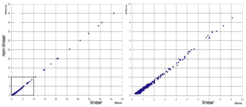
Comparison of peak heights between the linearly sampled 3.7-day experiment (horizontal) and the randomly sampled 12.7-hour experiment (vertical). The latter provides a high-fidelity reproduction of the peak heights in the full linearly sampled spectrum. Left: total range of peak heights of peaks. The region shown in the expansion on the right is indicated with a box. Right: expansion of the section containing weak peaks. Peaks were measured if they were larger than approximately 0.2 × 10⁹, which is approximately twice the amount of peak noise (see Fig. 5). Note that the values for the non-linearly sampled data are lower than those of the linearly sampled spectra by a constant offset of approximately the value of the peak noise.

Discussion

NMR spectra of mixtures of metabolites as obtained from cell extracts or other metabolomics samples contain a large number of signals, and high-resolution is needed in 2D spectra if one wants to resolve all signals. Since the metabolites have all narrow line widths the individual signals are resolvable in 2D NMR spectra but only when the experiments are sampled to long evolution times in the indirect dimension. Previously, we have argued signals should be recorded to about T₂* in order to obtain good resolution without significantly deteriorating signal to noise ²⁴. For spectra of metabolites with narrow line widths this requires sampling to long evolution times and needs very long measuring times. We have recorded a ¹H-¹³C HSQC spectrum with 8k by 2k (real) data points in the t₁ and t₂ dimensions, respectively. Estimating that the spectrum contains as many as 1000 cross peaks, each peak is defined by 32k data points in the average. Thus, the information content of linearly sampled data is large compared to the number of parameters needed to characterize the spectrum. Thus, it seems feasible to extract spectral parameters from a reduced data set, such as obtained with NLS.

The maximum t₁ value in the spectrum recorded here is 0.16 sec, which is still much less than the T₂ of ¹³C signals of most metabolites (> 1 sec). Spectral folding in the indirect dimension would allow reaching longer evolution times at reasonable overall duration of the experiments. Attempts towards this goal are in progress but have not been used initially for convenience of comparison with database spectra of metabolites. Spectral folding raises the question of whether the FM method can reproduce positive and negative signals. The procedure can handle this very well. Indeed we have obtained positive and negative peaks, and the reconstructed FIDs are complex. We phase correct the final spectrum after FFT of the reconstructed time domain data set.

We have developed a simple new algorithm that estimates missing time-domain data points of non-linearly sampled data by conjugate gradient minimization of the target function T(f), which is constructed from the negative Shannon entropy of the frequency spectrum, S(f). Here, the negative entropy is used as a convenient convex function that is efficient for minimizing the target function. It is essentially a norm of the frequency spectrum. The final spectrum reaches the minimum of the norm being consistent with the experimentally measured time-domain data points. We do not normalize the data points of the frequency spectrum, f_k, since they should not be considered probabilities. Thus, our approach differs from other Maximum entropy methods for NMR spectrum reconstruction ¹⁷, which pursue such normalization. Obviously, the Shannon entropy used here should not be confused with the thermodynamic or statistical entropy. Here we could use and have explored other convex functions to minimize the norm of the spectrum.

We have used zeros for the initial guesses of the missing data points. One could consider using other starting values. However, due to the oscillating nature of the free-induction decays, zero is in the center of the distribution of the possible expected values. We have explored using other starting values, such as using the values of adjacent measured points. This did not alter the outcome but typically extended the time to reach convergence.

We realize that experimental scientists often face situations where false minima are found in optimization procedures. We have examined different sampling schedules, which yielded almost identical results differing essentially only slightly in the noise level and the time it takes to reach convergence. Thus we think that there is little danger of being trapped in local minima. However, this is likely to depend on how many data points are sampled in relation to the complexity of the spectra, and further investigations of this aspect are to be pursued.

It is worth asking whether the FM reconstruction alters peak shapes as has been reported for other methods of reconstructing NLS data. This does not directly apply to the metabolite data presented here, however. Because of the very long carbon transverse relaxation times, peaks are defined by one or two data points only. Thus, no distortion has or can be seen in the type of data shown here. However, we have started to apply this method to protein NOESY spectra and do not see significant distortions of peak shapes as long as we have enough data points in the indirect dimensions to define all spectral parameters. This leads to the question of what is the minimum number of non-linearly sampled data points to faithfully reconstruct a spectrum. This depends on the type of spectrum, and the density of signals. A NOESY of a large protein with a long mixing time and many cross peaks will require more points than one of a small protein with a short mixing time.

By principle of design, the FM reconstruction algorithm presented here does not allow for variation of measured time-domain data points. Our hypothesis was that this feature would avoid deemphasizing weak signals as long as they are represented in the measured data points. The results shown here confirm that this is indeed the case. FM reconstruction does not require setting of parameters for the reconstruction. The only operator decision to be made is when to terminate the iterative minimization of the target function T(f). On the other hand, our FM reconstruction is not suitable for and cannot be applied to linearly sampled data sets. However, it could be used for correcting erroneous or lost data points. The final FM reconstruction result is a time-domain data set that can be transformed with any of the available processing programs, manipulated with apodization functions, or extended with linear prediction. Here we have used the NMRPipe software package ⁴⁵ for all processing.

While we have applied window functions to the final reconstructed time-domain data one could also consider doing this to the initial non-linearly sampled data. As the reconstruction method used here is deemed to be of non-linear nature, there is no warranty that the reconstruction yields exactly the same result in these two cases. However, because we are aiming for linear response of signals, the FM reconstruction has to be at least of near linear nature. This means that the FM reconstruction method should be nearly independent of whether window functions are applied before or after apodization. In other words, the result would be extremely similar, within the scope of setting stop criteria of the minimization routine, and in either case, apodization does not interfere with the core of the FM method.

So far, we have used FM reconstruction for processing spectra with only one non-linearly sampled indirect dimension. However, this approach should be applicable to nD data that are sampled non-linearly in more than one indirect dimension. Here we have used a standard conjugate gradient minimizer, and processing is relatively slow as reconstruction of one 4k complex time-domain data set with 6/7^th of the data points missing takes about 3 to 5 hours on an Opteron computer. Obviously, the processing time depends on the number of missing points, and shorter time domain data can be processed significantly faster. Processing of 2D spectra benefits for farming out the reconstruction of FIDs to processors of PC clusters. However, the current FM reconstruction is significantly slower than the MaxEnt routine used in the Rowland NMR Toolkit (RNMRTK), which uses an analytically calculated gradient for minimizing the target function.

In principle, it is possible to apply FM reconstruction to higher-dimensional spectra with more than one non-linearly sampled dimension, and efforts towards this aim are in progress.

References

- 1.Lindon JC, Holmes E, Nicholson JK. Curr Opin Mol Ther. 2004;6:265–72. [PubMed] [Google Scholar]
- 2.Nicholson JK, Lindon JC, Holmes E. Xenobiotica. 1999;29:1181–9. doi: 10.1080/004982599238047. [DOI] [PubMed] [Google Scholar]
- 3.El-Deredy W. NMR Biomed. 1997;10:99–124. doi: 10.1002/(sici)1099-1492(199705)10:3<99::aid-nbm461>3.0.co;2-#. [DOI] [PubMed] [Google Scholar]
- 4.Gavaghan CL, Wilson ID, Nicholson JK. FEBS Lett. 2002;530:191–6. doi: 10.1016/s0014-5793(02)03476-2. [DOI] [PubMed] [Google Scholar]
- 5.Weljie AM, Newton J, Mercier P, Carlson E, Slupsky CM. Anal Chem. 2006;78:4430–42. doi: 10.1021/ac060209g. [DOI] [PubMed] [Google Scholar]
- 6.Liang YS, Kim HK, Lefeber AW, Erkelens C, Choi YH, Verpoorte R. J Chromatogr A. 2006;1112:148–55. doi: 10.1016/j.chroma.2005.11.114. [DOI] [PubMed] [Google Scholar]
- 7.Keating KA, McConnell O, Zhang Y, Shen L, Demaio W, Mallis L, Elmarakby S, Chandrasekaran A. Drug Metab Dispos. 2006;34:1283–7. doi: 10.1124/dmd.105.008763. [DOI] [PubMed] [Google Scholar]
- 8.Dunn WB, Bailey NJ, Johnson HE. Analyst. 2005;130:606–25. doi: 10.1039/b418288j. [DOI] [PubMed] [Google Scholar]
- 9.Rhee IK, Appels N, Hofte B, Karabatak B, Erkelens C, Stark LM, Flippin LA, Verpoorte R. Biol Pharm Bull. 2004;27:1804–9. doi: 10.1248/bpb.27.1804. [DOI] [PubMed] [Google Scholar]
- 10.Frederich M, Cristino A, Choi YH, Verpoorte R, Tits M, Angenot L, Prost E, Nuzillard JM, Zeches-Hanrot M. Planta Med. 2004;70:72–6. doi: 10.1055/s-2004-815461. [DOI] [PubMed] [Google Scholar]
- 11.Barna JCJ, Laue ED. J Magn Reson. 1987;75:384–389. [Google Scholar]
- 12.Hoch JC, Stern AS, Donoho DL, Johnstone IM. J Magn Reson. 1990;86:236–246. [Google Scholar]
- 13.Barna JCJ, Laue ED, Mayger MR, Skilling J, Worrall SJP. J Magn Reson. 1987;73:69–77. [Google Scholar]
- 14.Burg J. Maximum entropy spectral analysis. In: Donald G, Childers D, editors. 37th Meeting of the Society for exploratory geophysics, 1967; New York: IEEE Press; 1967. 1978. [Google Scholar]
- 15.Hoch JC. Methods Enzymol. 1989;176:216–41. doi: 10.1016/0076-6879(89)76014-6. [DOI] [PubMed] [Google Scholar]
- 16.Delsuc MA. A New Maximum Entropy Processing Algorithm, with Applications to Nuclear Magnetic Resonance Experiments. In: Skilling J, editor. Maximum Entropy and Bayesian Methods. Kluwer Academic; Amsterdam: 1989. [Google Scholar]
- 17.Robin, Delsuc, Guittet E, Lallemand J Magn Reson. 1991;92:645–650. [Google Scholar]
- 18.Jones J, Hore P. J Magn Reson. 1991;92:276–292. [Google Scholar]
- 19.Jones J, Hore P. J Magn Reson. 1991;92:363–376. [Google Scholar]
- 20.Schmieder P, Stern AS, Wagner G, Hoch JC. J Biomol NMR. 1993;3:569–76. doi: 10.1007/BF00174610. [DOI] [PubMed] [Google Scholar]
- 21.Schmieder P, Stern AS, Wagner G, Hoch JC. J Biomol NMR. 1994;4:483–90. doi: 10.1007/BF00156615. [DOI] [PubMed] [Google Scholar]
- 22.Schmieder P, Stern AS, Wagner G, Hoch JC. J Magn Reson. 1997;125:332–9. doi: 10.1006/jmre.1997.1117. [DOI] [PubMed] [Google Scholar]
- 23.Li KB, Stern AS, Hoch JC. J Magn Reson. 1998;134:161–3. doi: 10.1006/jmre.1998.1514. [DOI] [PubMed] [Google Scholar]
- 24.Rovnyak D, Hoch JC, Stern AS, Wagner G. J Biomol NMR. 2004;30:1–10. doi: 10.1023/B:JNMR.0000042946.04002.19. [DOI] [PubMed] [Google Scholar]
- 25.Rovnyak D, Frueh DP, Sastry M, Sun ZY, Stern AS, Hoch JC, Wagner G. J Magn Reson. 2004;170:15–21. doi: 10.1016/j.jmr.2004.05.016. [DOI] [PubMed] [Google Scholar]
- 26.Sun ZJ, Hyberts SG, Rovnyak D, Park S, Stern AS, Hoch JC, Wagner G. J Biomol NMR. 2005;32:55–60. doi: 10.1007/s10858-005-3339-y. [DOI] [PubMed] [Google Scholar]
- 27.Sun ZY, Frueh DP, Selenko P, Hoch JC, Wagner G. J Biomol NMR. 2005;33:43–50. doi: 10.1007/s10858-005-1284-4. [DOI] [PubMed] [Google Scholar]
- 28.Frueh DP, Sun ZY, Vosburg DA, Walsh CT, Hoch JC, Wagner G. J Am Chem Soc. 2006;128:5757–5763. doi: 10.1021/ja0584222. [DOI] [PMC free article] [PubMed] [Google Scholar]
- 29.Tugarinov V, Kay LE, Ibraghimov I, Orekhov VY. J Am Chem Soc. 2005;127:2767–75. doi: 10.1021/ja044032o. [DOI] [PubMed] [Google Scholar]
- 30.Chylla RA, Markley JL. J Biomol NMR. 1995;5:245–58. doi: 10.1007/BF00211752. [DOI] [PubMed] [Google Scholar]
- 31.Marion D. J Biomol NMR. 2005;32:141–50. doi: 10.1007/s10858-005-5977-5. [DOI] [PubMed] [Google Scholar]
- 32.Korzhneva DM, Ibraghimov IV, Billeter M, Orekhov VY. J Biomol NMR. 2001;21:263–8. doi: 10.1023/a:1012982830367. [DOI] [PubMed] [Google Scholar]
- 33.Orekhov VY, Ibraghimov IV, Billeter M. J Biomol NMR. 2001;20:49–60. doi: 10.1023/a:1011234126930. [DOI] [PubMed] [Google Scholar]
- 34.Orekhov VY, Ibraghimov I, Billeter M. J Biomol NMR. 2003;27:165–73. doi: 10.1023/a:1024944720653. [DOI] [PubMed] [Google Scholar]
- 35.Gutmanas A, Jarvoll P, Orekhov VY, Billeter M. J Biomol NMR. 2002;24:191–201. doi: 10.1023/a:1021609314308. [DOI] [PubMed] [Google Scholar]
- 36.Kupce E, Freeman R. J Biomol NMR. 2004;28:391–5. doi: 10.1023/B:JNMR.0000015421.60023.e5. [DOI] [PubMed] [Google Scholar]
- 37.Kupce E, Freeman R. J Am Chem Soc. 2004;126:6429–40. doi: 10.1021/ja049432q. [DOI] [PubMed] [Google Scholar]
- 38.Hounsfield GN. Brit J Radiol. 1973;46:1016. doi: 10.1259/0007-1285-46-552-1016. [DOI] [PubMed] [Google Scholar]
- 39.Szyperski T, Wider G, JH B, Wuthrich K. J Am Chem Soc. 1993;115:9307–9308. [Google Scholar]
- 40.Kim S, Szyperski T. J Am Chem Soc. 2003;125:1385–93. doi: 10.1021/ja028197d. [DOI] [PubMed] [Google Scholar]
- 41.Liu G, Aramini J, Atreya HS, Eletsky A, Xiao R, Acton T, Ma L, Montelione GT, Szyperski T. J Biomol NMR. 2005;32:261. doi: 10.1007/s10858-005-7941-9. [DOI] [PubMed] [Google Scholar]
- 42.Schmieder P, Stern AS, Wagner G, Hoch JC. J Magn Reson. 1997;125:332–9. doi: 10.1006/jmre.1997.1117. [DOI] [PubMed] [Google Scholar]
- 43.Hoch JC, Stern AS. Methods Enzymol. 2001;338:159–78. doi: 10.1016/s0076-6879(02)38219-3. [DOI] [PubMed] [Google Scholar]
- 44.Polak E, Ribiere G. Rev Francaise Informate Recherche Operatonelle. 1969;3:35–43. [Google Scholar]
- 45.Delaglio F, Grzesiek S, Vuister GW, Zhu G, Pfeifer J, Bax A. J Biomol NMR. 1995;6:277–93. doi: 10.1007/BF00197809. [DOI] [PubMed] [Google Scholar]