Inferences and Power Analysis Concerning Two Negative Binomial Distributions with An Application to MRI Lesion Counts Data

Abstract

In comparing the mean count of two independent samples, some practitioners would use the t-test or the Wilcoxon rank sum test while others may use methods based on a Poisson model. It is not uncommon to encounter count data that exhibit overdispersion where the Poisson model is no longer appropriate. This paper deals with methods for overdispersed data using the negative binomial distribution resulting from a Poisson-Gamma mixture. We investigate the small sample properties of the likelihood-based tests and compare their performances to those of the t-test and of the Wilcoxon test. We also illustrate how these procedures may be used to compute power and sample sizes to design studies with response variables that are overdispersed count data. Although methods are based on inferences about two independent samples, sample size calculations may also be applied to problems comparing more than two independent samples. It will be shown that there is gain in efficiency when using the likelihood-based methods compared to the t-test and the ilcoxon test. In studies where each observation is very costly, the ability to derive smaller sample size estimates with the appropriate tests is not only statistically, but also financially, appealing.

1. INTRODUCTION

Magnetic Resonance Imaging (MRI) is a widely used tool in Multiple Sclerosis (MS), often to provide count data of abnormally appearing areas of the brain called lesions. These lesions do not occur in a manner consistent with either the Poisson distribution, usually used for count data, or normal distribution. In many cases, the mean is reasonably small, and overdispersion is observed across observations, and it is not predicted by the simple Poisson model. A typical solution to this problem is to consider the family of mixed Poisson distributions with probability mass function (pmf)

$$P(Y=y)={\int }_0^{\infty }\frac{e^{-\nu }{\nu }^y}{y!}f(\nu )d\nu ,y=0,1,\dots ,$$

where f(ν) is the known density of a mixture distribution for ν, where ν is the mean of the Poisson model. If we let f(ν) be a density of Gamma distribution, with scale parameter μ/ϑ and shape parameter ϑ, the resulting marginal distribution of the count random variable Y is a negative binomial distribution (NB), denoted by NB(μ, ϑ), with pmf

$$P(Y=y)=\frac{\mathrm{\Gamma }(y+\vartheta )}{\mathrm{\Gamma }(\vartheta )\mathrm{\Gamma }(y+1)}\frac{{\vartheta }^{\vartheta }{\mu }^y}{{(\vartheta +\mu )}^{(\vartheta +y)}},y=0,1,\dots ,\vartheta >0,\mu >0$$

where Γ(·) is the gamma function. In this case, the mean and variance of Y are E(Y) = μ and V(Y) = μ + μ²/ϑ, respectively. For a fixed μ, NB gets closer to Poisson as ϑ → ∞ (For additional discussions and applications of Poisson mixture models, readers may refer to Grandell (1997), Hougaard, Lee, and Whitmore (1997) and J. Lawless (1987).)

This paper is motivated by the problem of sample size and power calculations to design clinical trials in MS. The outcome variable of interest is the number of gadolinium enhanced lesions as obtained from MRI. The objective is to examine treatment effects measured by the change in the mean number of lesions based on the comparison of two independent groups. Most studies involving MRI lesion counts utilize the nonparametric Wilcoxon rank sum test in their analyses (cf., Nauta et al. (1994), Truyen et al. (1997), Tubridy et al. (1998)). Wilcoxon rank sum test is an alternative method to t-test for comparing two independent samples without assuming the samples came from normal distributions. This method is based on the ranks of the combined observations from the two samples and is known to be less powerful than its parametric analog. (For more details of this test procedure, see for instance Lehmann (1975).) Recently, the mixed Poisson family of distributions was considered to model lesion counts. In Sormani et al. (1999a, 1999b), they showed that negative binomial model gave a relatively good fit to this type of data. With an assumed parametric model, one may be able to develop more powerful tests and construct confidence intervals for treatment effect. Another important aspect in clinical trials is sample size and power calculations. In the late 1990’s, the nonparametric resampling method proposed by Nauta et al. (1994) was the method utilized by most researchers in this area to do power analysis (cf., Truyen et al. (1997), Tubridy et al. (1998), Sormani et al. (1999b)). Sormani et al. (2001b) proposed a parametric resampling method to compute sample size and power using historical data to estimate the parameters of the negative binomial distribution, and then employ the Wilcoxon rank sum test to evaluate the power. If the negative binomial distribution is an appropriate model for lesion counts data, parametric tests based on the negative binomial model will be shown to be more efficient, i.e., smaller sample size needed to achieve the same power.

In Section 2, we derive and investigate statistical inference methods for comparing two independent negative binomial distributions using the likelihood function. The goal is to help researchers understand the ideas behind the derived test procedures and choose the best method. In Section 3, we simulate the power and type I error rates of the likelihood-based procedures via Monte Carlo simulations, and compare them with the Wilcoxon two-sample test and the conventional t-test. In Section 4, we investigate the robustness of these tests when the assumption of common overdispersion parameter is violated. We illustrate how to numerically compute sample size and power of the likelihood-based method in Section 5. Finally, we provide an example using results from a clinical trial in MS in Section 6. We end the paper with some concluding remarks. For ease of reading, proofs are presented in the Appendix.

2. Tests and Confidence Intervals

Suppose that we have two independent random samples X₁,…, X_m with pmf NB(μ_X, ϑ_X) and Y₁,…, Y_n with pmf NB(μ_Y, ϑ_Y). Under this setting, let μ_X = μ and ϑ_X = ϑ and assume that μ_Y = γμ and ϑ_Y = ϑ, where μ, ϑ, and γ are positive-valued parameters. The assumption that ϑ_X = ϑ_Y is indeed a restriction but, as will be shown in Section 4, the likelihood-based methods are reasonably robust to this assumption.

We are interested in making inference about γ using likelihood methods. In clinical research, γ typically represents the treatment effect. If γ = 1, then we say that there is no evidence of a treatment effect. Otherwise, there is treatment effect. Although we assume that γ only affects μ and not ϑ, variance of Y is also affected by γ since V(Y) = γμ+γ²μ²/ϑ. For test of the hypothesis about γ, we consider the general case of testing H₀: γ = γ₀ versus H_a: γ ≠ γ₀. It should be noted that the negative binomial model considered in this paper no longer belongs to the exponential family of distributions because ϑ is unknown. However, it still satisfies the conditions (see for instance Bickel and Doksum (2001) pp. 384–385) necessary for the asymptotic results of likelihood-based inferences.

In the subsequent discussions, we use the notations: z_α to denote the (1−α)100^th percentile of a standard normal distribution, ${\chi }_{\alpha }^2(k)$ to denote the (1−α)100^th percentile of a chi squared distribution with k degrees of freedom, Ψ (·) to denote the digamma function and Ψ′ (·) to denote the trigamma function.

2.1. Generalized Likelihood Ratio Test

One of the popular methods for deriving statistical test procedures is based on the generalized likelihood ratio. For a vector of parameters θ∈Θ, the generalized likelihood ratio test (GLRT) for H₀: θ∈Θ₀ versus H_a: θ ∈ Θ− Θ₀ is defined as

$$\lambda (x,y)=\frac{sup\{L(\mathbf{x},\mathbf{y};\mathit{\theta }):\mathit{\theta }\in {\mathbf{\Theta }}_0\}}{sup\{L(\mathbf{x},\mathbf{y};\mathit{\theta }):\mathit{\theta }\in \mathbf{\Theta }\}}$$

where L(x, y;θ) is the likelihood function. We obtain sup{L(x, y; θ): θ ∈ Θ} by maximizing the likelihood, L(x, y; ϑ, μ, γ) or equivalently, the log likelihood under the unrestricted parameter space given by

$$\begin{array}{l}lnL(\mathbf{x},\mathbf{y};\vartheta ,\mu ,\gamma )=-(m+n)ln\mathrm{\Gamma }(\vartheta )+\sum _{i=1}^{m}ln\mathrm{\Gamma }(x_i+\vartheta )-\sum _{i=1}^{m}ln\mathrm{\Gamma }(x_i+1)\\ +\sum _{j=1}^{n}ln\mathrm{\Gamma }(y_j+\vartheta )-\sum _{j=1}^{n}ln\mathrm{\Gamma }(y_j+1)+(m+n)\vartheta ln\vartheta +(n\overline{y})ln\gamma \\ +(m\overline{x}+n\overline{y})ln\mu -m(\vartheta +\overline{x})ln(\vartheta +\mu )-n(\vartheta +\overline{y})ln(\vartheta +\gamma \mu )\end{array}$$ (2.1)

where m and n are the respective sample sizes of x and y. On the other hand, sup{L(x, y; θ): θ ∈ Θ₀} is obtained by maximizing the likelihood under H₀: γ = γ₀.

In the next two lemmas, we obtain the MLE under both the unrestricted and the restricted parameter spaces.

Lemma 1

Let X₁,…, X_m be iid random variables from NB(μ, ϑ) and Y₁, …, Y_n be iid random variables from NB(γμ, ϑ), where X_is and Y_js are independent. In the unrestricted parameter space Θ, the MLEs for μ and γ are μ̂ = x̄ and γ̂ = ȳ/x̄, respectively, and the MLE ϑ̂ for ϑ solves the equation

$$0=-(m+n)\mathrm{\Psi }(\widehat{\vartheta })+\sum _{i=1}^m\mathrm{\Psi }(x_i+\widehat{\vartheta })+\sum _{j=1}^n\mathrm{\Psi }(y_j+\widehat{\vartheta })+mln\left(\frac{\widehat{\vartheta }}{\widehat{\vartheta }+\overline{x}}\right)+nln\left(\frac{\widehat{\vartheta }}{\widehat{\vartheta }+\overline{y}}\right).$$ (2.2)

Lemma 2

Using the assumptions of Lemma 1, when γ = γ₀ is known, the MLE for μ₀ is given by

$$\begin{array}{l}{\widehat{\mu }}_0=\frac{\sqrt{{[m({\gamma }_0\overline{x}-{\widehat{\vartheta }}_0)+n(\overline{y}-{\gamma }_0{\widehat{\vartheta }}_0)]}^2+4{\widehat{\vartheta }}_0{\gamma }_0(m+n)(m\overline{x}+n\overline{y})}}{2{\gamma }_0(m+n)}\\ +\frac{m({\gamma }_0\overline{x}-{\widehat{\vartheta }}_0)+n(\overline{y}-{\gamma }_0{\widehat{\vartheta }}_0)}{2{\gamma }_0(m+n)}\end{array}$$ (2.3)

and the MLE ϑ̂₀ for ϑ₀ solves the equation

$$\begin{array}{l}0=-(m+n)\left[\mathrm{\Psi }({\widehat{\vartheta }}_0)-1\right]+\sum _{i=1}^m\mathrm{\Psi }(x_i+{\widehat{\vartheta }}_0)+\sum _{j=1}^n\mathrm{\Psi }(y_j+{\widehat{\vartheta }}_0)+mln\left(\frac{{\widehat{\vartheta }}_0}{{\widehat{\vartheta }}_0+{\widehat{\mu }}_0}\right)\\ +nln\left(\frac{{\widehat{\vartheta }}_0}{{\widehat{\vartheta }}_0+{\gamma }_0{\widehat{\mu }}_0}\right)-\frac{m({\widehat{\vartheta }}_0+\overline{x})}{{\widehat{\vartheta }}_0+{\widehat{\mu }}_0}-\frac{n({\widehat{\vartheta }}_0+\overline{y})}{{\widehat{\vartheta }}_0+{\gamma }_0{\widehat{\mu }}_0}.\end{array}$$ (2.4)

Using the results of these lemmas, we now obtain the Generalized Likelihood Ratio Test (GLRT) and corresponding confidence interval for γ.

Theorem 3

Define the generalized likelihood ratio statistic as

$${\chi }_L^2=-2ln\lambda =-2[lnL(\mathbf{x},\mathbf{y};{\widehat{\mu }}_0,{\widehat{\vartheta }}_0,{\gamma }_0)-lnL(\mathbf{x},\mathbf{y};\widehat{\mu },\widehat{\vartheta },\widehat{\gamma })],$$

where γ₀ is known, the function ln L(x, y; μ, ϑ, γ) is defined in (2.1) and μ̂₀, ϑ̂₀, μ̂, ϑ̂, and γ̂ are defined in Lemmas 1 and 2. Under the conditions defined in Lemma 1 and Lemma 2,

1. an approximate α-level test for H₀: γ = γ₀ versus H_a: γ ≠ γ₀ rejects H₀ when ${\chi }_L^2>{\chi }_{\alpha }^2(1)$; and

2. an approximate (1−α)100% confidence interval for γ is the set of γ₀ values such that $p-\mathit{value}=P\{{\chi }_L^2>{\chi }_{\alpha }^2(1)\}\ge \alpha$.

2.2. Wald’s Test

Another likelihood-based test, known as the Wald’s test, utilizes the large-sample properties of the MLE which we present in the next theorem. We first derive Wald’s inference procedures about γ using the properties of γ̂.

Theorem 4

Under the conditions defined in Lemma 8 in the Appendix, Z_{W I} = (γ̂ − γ)/σ̂_γ̂ has an asymptotic standard normal distribution where

$${\widehat{\sigma }}_{\widehat{\gamma }}=\sqrt{{\widehat{\sigma }}_{\widehat{\gamma }}^2}=\sqrt{\frac{\overline{y}[m\overline{x}(\widehat{\vartheta }+\overline{y})+n\overline{y}(\widehat{\vartheta }+\overline{x})]}{mn\widehat{\vartheta }{\overline{x}}^3}}.$$ (2.5)

Consequently,

1. an approximate α-level test for H₀: γ = γ₀ versus H_a: γ ≠ γ₀ rejects H₀ when ${\chi }_{WI}^2>{\chi }_{\alpha }^2(1)$, where

$${\chi }_{WI}^2={\left(\frac{\widehat{\gamma }-{\gamma }_0}{{\widehat{\sigma }}_{\widehat{\gamma }}}\right)}^2=\frac{{[(\overline{y}/\overline{x})-{\gamma }_0]}^2}{{\widehat{\sigma }}_{\widehat{\gamma }}^2}.$$

1. an approximate (1−α)100% confidence interval for γ is the set of γ₀ values such that $p-\mathit{value}=P\{{\chi }_{WI}^2>{\chi }_{\alpha }^2(1)\}\ge \alpha$, or equivalently, γ̂ ± z_α/2 σ̂_γ̂.

We also consider Wald-type procedures based on a differentiable monotonic function, g(γ), for γ > 0, for the purpose of stabilizing the variance of γ̂. In the next section, we will consider a few transformations and choose the best based on the simulated type I error rates and power levels, particularly in the case of small sample and more overdispersed data. Using the Delta Method and Slutsky’s theorem, it can easily be shown that Z_Wg = [g(γ̂) − g(γ)]/[g′(γ̂) σ̂_γ̂] has an asymptotic standard normal distribution where γ̂ = ȳ/x̄ and σ̂_γ̂ is as defined in equation (2.5). Thus, an approximate α-level test for H₀: g(γ) = g(γ₀) versus H_a: g(γ) ≠ g(γ₀) rejects H₀ when ${\chi }_{W_g}^2>{\chi }_{\alpha }^2(1)$, where

$${\chi }_{W_g}^2={\left[\frac{g(\widehat{\gamma })-g({\gamma }_0)}{g^{\prime }(\widehat{\gamma }){\widehat{\sigma }}_{\widehat{\gamma }}}\right]}^2,$$

and an approximate (1 − α)100% confidence interval g(γ) is given by g(γ̂) ± z_α/2 g′(γ̂) σ̂_γ̂. If we let U_g and L_g denote, respectively, the upper and lower confidence limits of this interval, then an approximate (1 − α)100% CI for γ based on g(γ̂) is given by [g⁻¹(U_g), g⁻¹ L_g)].

2.3. Score Test

The third likelihood-based inference method is called the score or Rao’s test, which utilizes the asymptotic property of the vector of score statistics, U(θ), defined as the vector of partial derivatives of the likelihood function with respect to the parameters, i.e., U(θ) = ∂ ln L(x, y; θ)/∂θ. From large-sample theory of score statistics (c.f., Cox and Hinkley (1974)), U(θ)′Σ(θ)U(θ), where Σ(θ) is defined in equation (8.2) in the Appendix, converges to a multivariate normal distribution. The next theorem applies this asymptotic result to the setting of interest.

Theorem 5

Under the conditions defined in Lemma 2, an approximate α-level test for H₀: γ = γ₀ versus H_a: γ ≠ γ₀ rejects H₀ when ${\chi }_S^2>{\chi }_{\alpha }^2(1)$ where

$${\chi }_S^2=\frac{{(\overline{y}-{\widehat{\mu }}_0{\gamma }_0)}^2}{{({\widehat{\vartheta }}_0+{\gamma }_0{\widehat{\mu }}_0)}^2}\left\{\frac{n{\widehat{\vartheta }}_0[m({\widehat{\vartheta }}_0+{\gamma }_0{\widehat{\mu }}_0)+n{\gamma }_0({\widehat{\vartheta }}_0+{\widehat{\mu }}_0)]}{m{\gamma }_0{\widehat{\mu }}_0}\right\}$$

and ϑ̂₀ and μ̂₀ are defined in equations (2.4) and (2.3). Moreover, the set of γ₀ values such that $p-\mathit{value}=P\{{\chi }_S^2>{\chi }_{\alpha }^2(1)\}\ge \alpha$ gives an approximate (1 − α)100% confidence interval for γ.

Remark 6

For Wald’s and score tests, one may easily modify the tests to derive procedures to test H₀: γ ≤ γ₀ versus H_a: γ > γ₀, or H₀: γ ≥ γ₀ versus H_a: γ < γ₀, based on the test statistics

$$Z_{WI}=\frac{\widehat{\gamma }-{\gamma }_0}{{\widehat{\sigma }}_{\widehat{\gamma }}}(\text{Wal}{\text{d}}^{\prime }\text{s}\text{test})$$

and

$$Z_S=\frac{(\overline{y}-{\widehat{\mu }}_0{\gamma }_0)}{({\vartheta }_0+{\gamma }_0{\mu }_0)}\sqrt{\frac{n{\widehat{\vartheta }}_0[m({\widehat{\vartheta }}_0+{\gamma }_0{\widehat{\mu }}_0)+n{\gamma }_0({\widehat{\vartheta }}_0+{\widehat{\mu }}_0)]}{m{\gamma }_0{\widehat{\mu }}_0}}(\text{score}\text{test}),$$

using standard normal (z_α) instead of chi squared critical values. Similarly, we can derive the one-sided Wald-type test based on Z_Wg.

Remark 7

The p-values of the Wald’s and GLRT discussed here may also be obtained in SAS via PROC GENMOD using a generalized linear model (GLM) assuming a negative binomial distribution with common overdispersion parameter and a natural logarithm link function. Given a covariate W, the mean μ of a negative binomial is related to W via the equation

$$log\mu ={\beta }_0+{\beta }_{1}W,\text{so}\text{that}\mu =exp\{{\beta }_0+{\beta }_{1}W\}.$$

In the current setting, W is a dichotomous variable where W = 1 if the subject belongs to one treatment group and W = 0 if the subject belongs to the other treatment group. The results of the likelihood ratio methods (tests and confidence intervals) for γ and β₁ are equivalent, and one can get the interval for one parameter from the other parameter using the relation γ = exp{β₁}. By default, PROC GENMOD provides test results and confidence intervals based on GLRT. However, GENMOD also provides results based on Wald’s procedures for β₁ which are equivalent to the Wald’s method presented in this paper for g(γ) = log γ. With regard to ϑ, the overdispersion parameter in GENMOD is defined as 1/ϑ.

3. Small Sample Properties

From theory, the likelihood-based inference methods (GLRT, Wald’s and score) obtained in the previous section are equivalent in the large-sample case. In small samples, their performances are different. The small sample distributional properties of these tests are difficult to investigate analytically so we instead performed Monte Carlo simulations. Furthermore, we compared the performance of the likelihood-based tests with two of the most popular methods used to compare means of two independent samples – the nonparametric Wilcoxon rank sum test and the two sample t-test assuming unequal variance. Our objective in this section is to determine the best test procedure under the setting of the simulations performed.

We considered the typical case of interest in practice which is testing H₀: γ = 1 versus H_a: γ ≠ 1, i.e., testing if there is enough evidence to conclude that the mean counts of the two groups are different, at 5% level of significance. Note that in using Wald’s test procedures based on g(γ), these hypotheses are equivalent to H₀: g(γ) = g(1) versus H_a: g(γ) ≠ g(1). For convenience, we generated two independent negative binomial random samples X₁, …, X_n and Y₁,…, Y_n of equal sizes (denoted by n) for selected values of the parameters γ, μ and ϑ and applied the test procedures. We repeated this process 10,000 times. We obtained the simulated type I error rate and the simulated power of each test by computing the percentage of times out of the total replicates the null hypothesis was rejected when γ = 1 and γ ≠ 1, respectively. We chose values of μ and ϑ that mimic samples from an overdispersed model. Simulations and computations were coded in Fortran language utilizing subroutines in IMSL Fortran Libraries and graphs were generated using S-Plus. We only present a subset of the simulations we have performed.

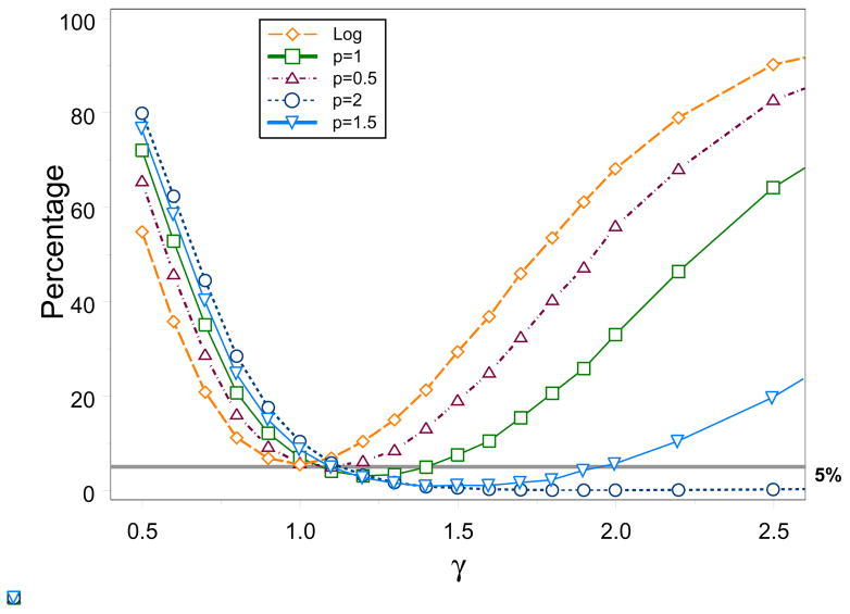
Our first goal is to choose the best Wald-type test considering the following g functions: g(γ) = log γ and g(γ) = γ^p for p ∈ {0.5, 1, 1.5, 2}. When p = 1, we get the standard test based on Z_{W I}. Figure 1 shows the simulated power for varying values of γ when n = 50, μ = 1 and ϑ = 0.75. We desire power levels to be as high as possible under the alternative hypothesis. Except for the log-transformed test, we observe that the levels of the tests based on g(γ) = γ^p fall below the 5% line for γ > 1, and the range of γ for which this occurs gets larger as p increases. If we choose the test associated with p = 2, it has the highest power to detect γ values less than 1 but has power values near 0 even at γ = 2.5 and highest type I error rate (i.e., level at γ = 1). One can go around this problem by labeling the two groups such that the γ̂ < 1. However, the performance of a two-sided test for H₀: γ = 1 should not depend on the labeling of the groups. We attribute this weakness to the severely skewed distribution and unstable variance of γ̂. Although the log function has the smallest power for γ < 1, its power is comparable to the other tests while it outperforms all the other tests for γ > 1. Furthermore, its type I error rate is at about 5%. Taking the log pulls the large values of γ̂ closer to the smaller values and, thus, helps make the distribution more symmetric and the variance more stable. Note that the test when p = 0.5 (i.e., square-root transformation) also performs reasonably well and we expect any tests with p < 0.5 to result in further improvement. Instead of searching for the best value of p, we choose the log transformation because of its consistently good performance in both type I error and power and it is also coincides with Wald’s test used in generalized linear models for negative binomial. In the subsequent discussions, the Wald’s test is the test about log γ.

Figure 1.

Simulated power levels (in %) of Wald-type tests for varying values of γ when n = 50, ϑ = 0.75, and μ = 1.

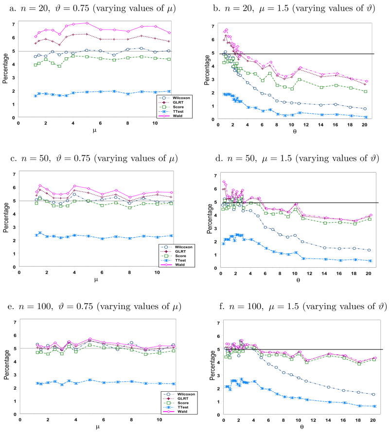
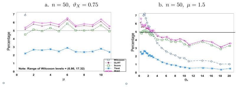
Next we compare the likelihood-based tests, t-test and Wilcoxon test with respect to type I error rates and power. Figure 2 gives the simulated type I error rates for varying values of μ and ϑ when n ∈ {20, 50, 100}. We desire tests with simulated type I error rates below and as close to the set significance level α = 0.05 as possible. Levels for all tests get closer to 5% as sample size increases except for the t-test which remains at about the same level in all cases considered. The conservative nature of the t-test is due to its overestimation of the variance of γ̂, attributed to the few large observations on the tail of a heavily right-skewed negative binomial distribution, resulting in smaller values of the test statistic. There are no obvious trends in the levels for varying values of μ, but there is an evident decreasing trend in the error rates of all tests as ϑ increases and then eventually flattens out. Wald’s test and GLRT have rates above 5% for small n. The levels of score and Wilcoxon tests, even for small n, are near or below the target 5%. For n = 100 or more, levels for the likelihood-based tests are practically the same.

Figure 2.

Simulated Type I Error Rates (in %).

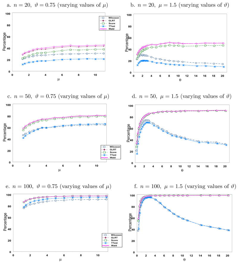
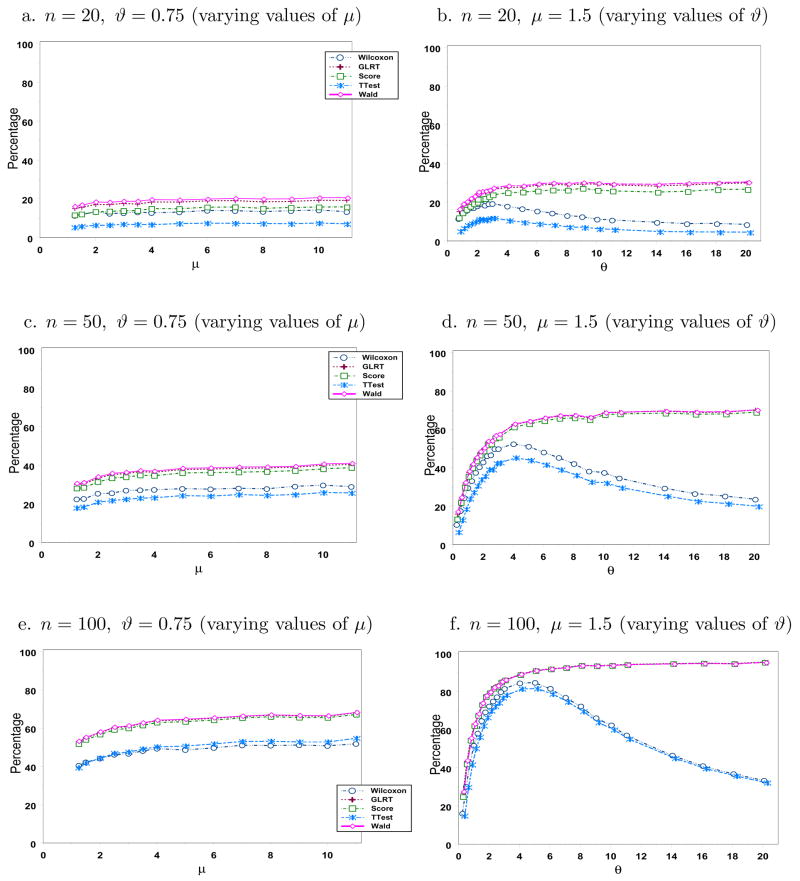
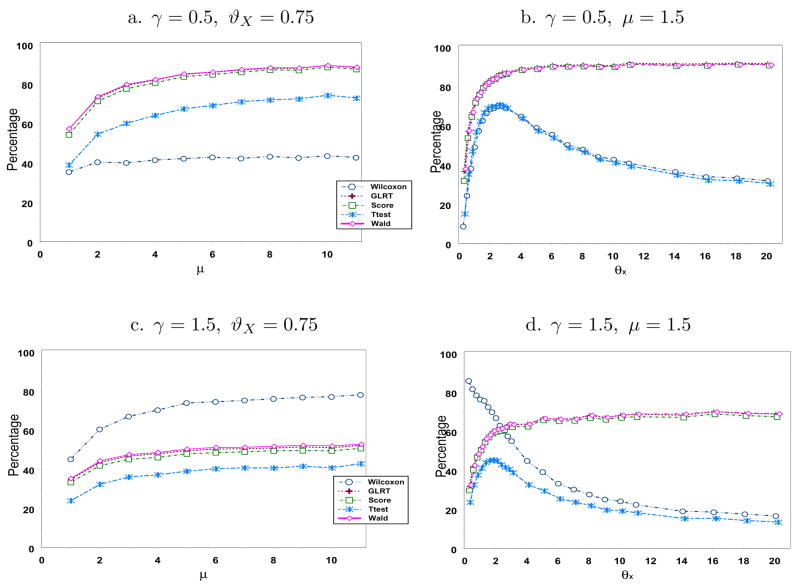
Figures 3 and 4 display the simulated power using the same parameters as in Figure 2 with γ ∈ {0.5, 1.5}, respectively. Although not presented, we also looked at other values of γ and arrived at similar conclusions. As expected, power increases as n increases for all cases. Wald’s test has the highest power, which is not surprising given that it also has the highest type I error rate. Wilcoxon test has the lowest power as it relies only on the ranks of the observations. Although both the mean and the variance increase as μ increases for a fixed ϑ, our simulation results show that power increases with μ for the range of values considered when ϑ = 0.75. The story is quite interesting when one varies ϑ fixing μ at 1.5. The likelihood-based tests perform very well and have power values which increase with ϑ. However, the power levels of the t-test and of the Wilcoxon test show power functions that increase up to some point as ϑ increases. This pattern is very evident when n is large. Recall that the limiting distribution of a negative binomial when ϑ → ∞ is Poisson. Hence, we expect this decrease to flatten out at a certain point as verified by our simulation when we looked at larger values of ϑ (results not presented here). One can then conclude gain in efficiency in using likelihood-based methods over t-test and the Wilcoxon test in this setting.

Figure 3.

Simulated power levels (in %)when γ = 0.5.

Figure 4.

Simulated power levels (in %)when γ = 1.5.

These simulation results support the use of likelihood-based methods over t-test and Wilcoxon test if the negative binomial, or even the Poisson model, is believed to be appropriate. For small values of n, μ, and ϑ, the score test is recommended because its type I error rate is expected to be close to or lower than the set significance level and has reasonable power. For moderate sample sizes (> 50) or small n but relatively large (> 5), we recommend GLRT or Wald’s test because they are more efficient, at the same time having acceptable type I error rates.

4. Robustness to the Common Dispersion Assumption

In this section, we investigate the robustness of the likelihood-based methods, t-test and Wilcoxon test to the assumption that ϑ is the same for the two treatment groups. SAS PROC GENMOD also uses this assumption in modeling overdispersed count data using negative binomial distribution in a general linear model setting. The common overdispersion parameter plays a critical role when overdispersion is more pronounced, i.e., for small values of ϑ. As ϑ increases, the effects of overdispersion and of the assumption of equal overdispersion parameter decrease, as will be seen in our simulation results. We follow the basic simulation process performed in the preceding section. We generated two independent random samples X₁, …, X_n ~ NB(μ, ϑ_X) and Y₁, …, Y_n ~ NB(γμ, ϑ_Y) where ϑ_Y = ηϑ_X for η > 1.

Figure 5 display the simulated type I error rates for n = 50 and η = 2 and selected values of μ and ϑ_X. The likelihood-based tests and the t-test have slightly higher type I error rates than the ϑ_X = ϑ_Y case but not much different. The Wilcoxon test is affected the most by the violation of this assumption. Its error rates as a function of μ, which range from [6.86, 17.32] when ϑ_X = 0.75, lie mostly outside our window but its curve actually shows an increasing trend as μ increases. Because this test depends on the ranks of the combined observations, it will be more sensitive to any change in the ordering of the data from the two treatment groups, and hence, increases the type I error rate. Increasing ϑ_Y by a factor of η > 1 relative to ϑ_X will result in less overdispersed Y_is. Therefore, Y_is will have less extreme observations and, consequently, will be assigned lower ranks than the X_is. This will then be detected by the Wilcoxon test. Note that if we look at the simulated error rates as a function of ϑ_X, all levels (including that of Wilcoxon test) decrease as ϑ_X increases and mimic the behavior under ϑ_X = ϑ_Y.

Figure 5.

Simulated Type I Error Rates (in %) when n = 50 and ϑ_Y = 2ϑ_X.

The simulated power levels are displayed in Figure 6 for γ ∈ {0.5, 1.5}, n = 50 and η = 2. The levels are again slightly higher for the t-test and the likelihood-based tests when compared to the levels in Figures 3 and 4 for n = 50. This behavior is expected due to the higher type I error rates. Fixing ϑ_X = 0.75, the Wilcoxon test is the least powerful when γ = 0.5, but most powerful when γ = 1.5. We can attribute this behavior to the interplay between the means and the overdispersion parameter. In the former case, μ_Y = 0.5μ_X compensates for the fact that ϑ_Y = 2ϑ_X. In the latter case, μ_Y = 1.5μ_X and ϑ_Y = 2ϑ_X will result in larger Y_i values and more extreme observations. We see similar patterns if we vary ϑ_X in the range (0, 2). Note that for values of ϑ_X > 10, the behavior of all tests mimic their behavior under the setting where ϑ_X = ϑ_Y is true.

Figure 6.

Simulated power levels (in %) when n = 50 and ϑ_Y = 2 * ϑ_X.

As to be expected, the differences observed under the case where η = 2 are magnified for η > 2, especially for small ϑ_X, and are diminished for η < 2. The patterns for other sample sizes n are generally the same as that for n = 50. For smaller n, the error (power) curves are higher (lower) and more variable. For larger n, all curves are tighter with error curves closer to the 5% level and power curves higher.

For the cases considered in our simulation, we conclude that the likelihood-based methods perform well for testing equality of mean counts modelled by a negative binomial distribution, even when the overdispersion parameter of one group is twice that of the other group.

5. Power Analysis via Monte Carlo Simulation

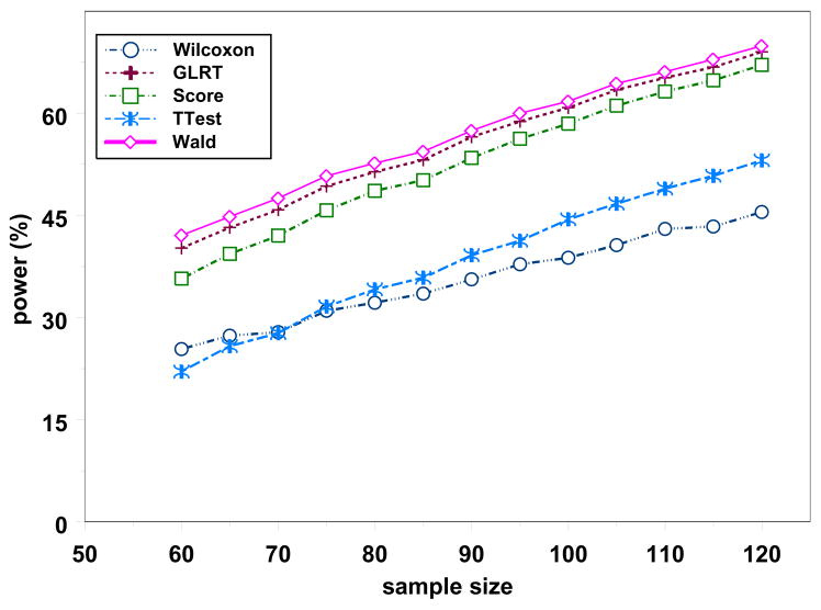
Because of the lack of closed form expressions for likelihood-based tests, we performed power analysis via parametric resampling based on a negative binomial distribution. This method is the same as the Monte Carlo method used in the previous section to simulate the power function with parameter values estimated from historical data as proposed in Sormani et al. (2001b). The power corresponding to the method used in the referenced paper would be the power under the Wilcoxon test. To illustrate our proposed method, suppose previous studies suggest μ = 1.65 and ϑ = 0.26, and we desire to detect a reduction of at least 60% in the mean count (i.e., γ = 1 – 0.6 = 0.4). We ran a total of 10,000 replications. Figure 7 displays the simulated power for varying values of n. When there are 80 observations per group, the estimated power for the Wilcoxon and t-tests are 32% and 34%, respectively, while the estimated power of the GLRT, score and Wald’s tests are 51%, 49% and 53%. Hence there is much gain in power from using any of these likelihood-based methods to achieve the same objective.

Figure 7.

Power Analysis using Monte Carlo simulations when γ = 0.4, ϑ = 0.26, and μ = 1.65.

Although the case considered here compares only two independent groups, one may still use the proposed method to compute power or sample size for more than two groups by applying the proposed methods to the pair that is either most relevant to the research hypothesis or to the pair that is expected to have the least difference or largest variance (to be more conservative). To address the issue of inflating the type I error rate due to multiple comparisons, one would need to adjust the overall significance level, α. The most popular method is the Bonferroni adjustment, which divides α by the number of pairwise comparisons to be made. For instance, if there are three treatment groups, say A, B and C, and it is of interest to do all pairwise comparisons (a total of 3 pairs), then the level of significance to be used in the power analysis or sample size calculation is 0.05/3 = 0.0167, instead of 5%. Using smaller significance level will result in higher sample size, which makes sense given that there are now more than two groups to compare.

6. Application

Recall that the motivation of this paper is to compare the contrast enhancing lesions, or so-called gadolinium (gad) lesions, from the MRI results of patients diagnosed with MS across two groups (active and placebo treatment). Gadolinium is an enhancement agent given to patients prior to MRI that enables inflammation and breaks in the blood brain barrier to be visualized on MRI. These areas of active inflammation are indicative of active disease and have been shown to be responsive to various immunomodulating treatments. Although these lesions have not been proven to be surrogate endpoints, they do enable an assessment of treatment effects on the inflammatory process and are widely used as outcome and safety measures in trials of relapsing remitting MS.

We apply the methods in this paper to an actual dataset from a study reported by Rudick et al. (2001). This study looked at the long term follow-up of all patients treated for at least two years in the original FDA Pivotal Trial of the drug Avonex compared to a placebo. Each patient considered for this comparison was enrolled in the Pivotal Trial and assigned either Avonex (Interferon β-1a) or placebo. The study was terminated early for efficacy based on time until sustained worsening in disability so that not all patients were eligible for a two year examination. In the design, MRIs were taken yearly. Among those patients who were eligible for a two year examination, only patients with MRI assessments for enhancing lesions at baseline and year 2 were included in these comparisons (81 out of 85 patients in the Avonex group and 82 out of 87 in the placebo group). Table 1 presents summary statistics of these data. The MLEs for γ, μ, and ϑ were found to be γ̂ = 0.495, μ̂ = 1.646, and ϑ̂ = 0.256.

Table 1.

Summary Statistics of the Number of Lesions

Group	Sample Size	Median	Max	Mean	Std Dev
Placebo	82	0.00	34	1.646	4.375
Avonex	81	0.00	13	0.815	2.044

One might wonder the consequences of not adjusting for overdispersion. Hence, we also performed a GLRT based on the Poisson assumption using SAS PROC GENMOD. Table 2 gives the results of all tests. The Poisson model substantially underestimates the variance, especially when ϑ and μ are small, as is the case in this example. Hence, it is not surprising that the Poisson test yielded a highly significant result with a GLRT p-value < 0.0001. Among the NB likelihood-based tests, GLRT and Wald’s test show significant differences at 5%, while the score test almost achieved significance. The Wilcoxon test has the largest p-value but still close to 5%. Given that n > 50 in this case, we would recommend the use of the GLRT or Wald’s test over the other tests. Therefore, we conclude that there is evidence of differences in mean lesion counts for patients in the treatment group compared to those in the placebo group.

Table 2.

Results of Tests

	Method
	Wilcoxon	GLRT(NB)	Wald(NB)	Score(NB)	T-test	GLRT(Poisson)
Test Stat	1.849	4.036	4.18	3.734	1.557447	23.2
p-value	0.0644	0.0445	0.0401	0.0533	0.1221	< 0.0001

Next we illustrate the methods for constructing an approximate confidence interval for γ by inverting the three likelihood-based tests. An approximate 95% confidence intervals for γ using GLRT, Wald’s test and score test are (0.25, 0.982), (0.252, 0.971) and (0.247, 1.011), respectively. Consistent with the results of the tests, the corresponding 95% confidence interval for γ based on Wald’s test and GLRT have values strictly less than 1, while the interval based on the score test contains the value 1. Using the interval based on Wald’s test, which is the narrowest, we estimate the percent reduction in average lesion count for the Avonex group, relative to the placebo group, to be between 2.9% [(1 − 0.971) * 100] to 74.8% [(1 − 0.252) * 100]. This interval is too wide to be informative for practical purposes. In order to have narrower confidence intervals, larger sample sizes for each treatment group are needed.

Finally, we checked if the assumptions we made about the model are reasonable. For each treatment group, we computed the MLEs of a 1-sample NB and Poisson models. We performed chi squared goodness-of-fit tests, as displayed in Table 3 using the intervals x = 0, 1, 2 and x ≥ 3. There is no evidence of a problem with fitting a negative binomial model to data on the treatment group while it is acceptable at 1% significance level for the placebo group. As expected, Poisson is clearly a bad fit to the data. We also constructed an approximate 95% confidence interval for ϑ for each sample by using Wald’s method. The resulting interval for the Avonex group is (0.256, 0.292), while the interval for the placebo group is (0.218, 0.238). These intervals do not overlap, implying that ϑ for the two groups are significantly different. However, the largest ratio between these two intervals is 1.34 (= 0.292/0.218). Based on the results in Section 4, the likelihood-based methods should still be applicable in this case.

Table 3.

Goodness-of-fit Statistics

	Poisson		Negative Binomial
	Test Stat	p-value	Test Stat	p-value
Placebo	355.23	< 0.0001	5.36	0.0206
Avonex	27.64	< 0.0001	0.46	0.4988

7. Conclusions

The likelihood-based methods to compare two NB distributions presented in this paper provide reasonably straightforward ways to handle overly dispersed count data. These methods were shown to be more efficient than the Wilcoxon and t-tests. Among the three likelihood-based methods, the score test was shown to perform the best for samples less than 50. For larger samples or less overdispersion, all three likelihood-based methods perform almost about the same in terms of type I error but Wald’s and GLRT provide higher power. In studies such as the one described in this paper, where each observation costs over $1000 per MRI, the ability to derive smaller sample size estimates with the appropriate tests is not only statistically, but also financially, appealing. While the purpose of this example is to illustrate the inferential methods based on negative binomial distribution, ideally we would like to have more frequent MRIs on each patient, such as monthly or quarterly. This will help reduce the number of false negatives, i.e., individuals who actually have enhancing lesions that are likely to be missed when less frequent MRIs are obtained. Also, multiple MRIs provide better estimates of the parameters which, as was shown by Sormani et. al. (2001b), reduces the sample size. Thus, there is an inherent trade off between cost and information which can be more precisely estimated given these improved parametric methods.

8. Appendix – PROOFS

Proof of Lemma 1

We first obtain the MLE for γ by taking the partial derivative of (2.1) with respect to γ

$$\frac{\partial lnL(\mathbf{x},\mathbf{y};\vartheta ,\mu ,\gamma )}{\partial \gamma }=\frac{n\overline{y}}{\gamma }-\frac{n\mu (\vartheta +\overline{y})}{\vartheta +\gamma \mu }=\frac{n\vartheta (\overline{y}-\mu \gamma )}{\gamma (\vartheta +\gamma \mu )}$$

Setting this to zero and solving, we get [nϑ̂ (ȳ − μ̂ γ̂)]/[γ̂ (ϑ̂ + γ̂μ̂)] = 0 so that γ̂ = ȳ/μ̂. Secondly, we take the partial derivative with respect to μ

$$\frac{\partial lnL(\mathbf{x},\mathbf{y};\vartheta ,\mu ,\gamma )}{\partial \mu }=\frac{m\overline{x}+n\overline{y}}{\mu }-\frac{m(\vartheta +\overline{x})}{\vartheta +\mu }-\frac{n\gamma (\vartheta +\overline{y})}{\vartheta +\gamma \mu }$$ (8.1)

Setting this to zero, using the result that γ̂ = ȳ/μ̂, and simplifying, we get μ̂ = x̄. Consequently, γ̂ = ȳ/x̄.

Finally, the partial derivative with respect to ϑ may be written as

$$\begin{array}{l}\frac{\partial lnL(\mathbf{x},\mathbf{y};\vartheta ,\mu ,\gamma )}{\partial \vartheta }=-(m+n)[\mathrm{\Psi }(\vartheta )-1]+\sum _{i=1}^m\mathrm{\Psi }(x_i+\vartheta )+\sum _{j=1}^n\mathrm{\Psi }(y_j+\vartheta )\\ +mln\left(\frac{\vartheta }{\vartheta +\mu }\right)+nln\left(\frac{\vartheta }{\vartheta +\gamma \mu }\right)-\frac{m(\vartheta +\overline{x})}{\vartheta +\mu }-\frac{n(\vartheta +\overline{y})}{\vartheta +\gamma \mu }.\end{array}$$

Setting this equation to zero, substituting μ̂ = x̄ and γ̂ = ȳ/x̄, and simplifying, we get (2.2).

Proof of Lemma 2

Under H₀: γ= γ₀, the log of the likelihood is (2.1) where γ, μ, and ϑ are replaced by γ₀, μ₀ and ϑ₀. We want the MLE for μ₀ and ϑ₀. Using the partial derivative function with respect to μ given by (8.1) and setting it equal to zero, we get

$$0=\frac{m\overline{x}+n\overline{y}}{{\mu }_0}-\frac{m({\vartheta }_0+\overline{x})}{{\vartheta }_0+{\mu }_0}-\frac{n{\gamma }_0({\vartheta }_0+\overline{y})}{{\vartheta }_0+{\gamma }_0{\mu }_0}$$

Simplifying, the above equation is equivalent to solving the equation

$$-{\mu }_0^2{\gamma }_0(m+n)+{\mu }_0[m(\overline{x}{\gamma }_0-{\vartheta }_0)+n(\overline{y}-{\gamma }_0{\vartheta }_0)]+{\vartheta }_0(m\overline{x}+n\overline{y})=0.$$

Using the quadratic formula and the fact that μ₀ > 0, we get (2.3). Next consider the partial derivative function with respect to ϑ as derived in the proof of Lemma 1. Substituting γ₀ for γ, μ̂₀ for μ and ϑ̂₀ for ϑ, (2.4) follows. Therefore, the MLEs for μ₀ and ϑ₀ for a given γ₀ solve equations (2.3) and (2.4).

Proof of Theorem 3

The proof follows immediately from the basic theory of the Generalized Likelihood Ratio Test, (see, for instance, Theorem 6.3.1 p. 394 of Bickel and Doksum (2001)) stating that −2 ln λ has an asymptotic χ² distribution with one degree of freedom. The corresponding asymptotic confidence interval method is obtained by inverting the GLRT.

Lemma 8

Let θ = (γ, μ, ϑ) and θ̂ = (γ̂, μ̂, ϑ̂) where γ̂, μ̂, and ϑ̂ are the MLEs obtained in Lemma (1). Under the conditions defined in Lemma 1 θ̂, with mean vector E(θ̂) = θ and variance-covariance matrix

$$\mathbf{\sum }(\mathit{\theta })=\left(\begin{array}{ccc}{\sigma }_{\widehat{\gamma }}^2& {\sigma }_{\widehat{\mu }\widehat{\gamma }}& 0\\ {\sigma }_{\widehat{\mu }\widehat{\gamma }}& {\sigma }_{\widehat{\mu }}^2& 0\\ 0& 0& {\sigma }_{\widehat{\vartheta }}^2\end{array}\right),$$ (8.2)

has an asymptotic multivariate normal distribution, where

$$\begin{array}{l}{\sigma }_{\widehat{\gamma }}^2=\frac{\gamma [m(\vartheta +\gamma \mu )+n\gamma (\vartheta +\mu )]}{mn\vartheta \mu };{\sigma }_{\widehat{\mu }}^2=\frac{\mu (\vartheta +\mu )}{m\vartheta };{\sigma }_{\widehat{\mu }\widehat{\gamma }}=\frac{-\gamma (\vartheta +\mu )}{m\vartheta };\\ {\sigma }_{\widehat{\vartheta }}^2={\left\{(m+n){\mathrm{\Psi }}^{\prime }(\vartheta )-\frac{\mu }{\vartheta }\left(\frac{m}{\vartheta +\mu }+\frac{n\gamma }{\vartheta +\gamma \mu }\right)-\sum _{i=1}^m\text{E}[{\mathrm{\Psi }}^{\prime }(x_i+\vartheta )]-\sum _{j=1}^n\text{E}[{\mathrm{\Psi }}^{\prime }(y_j+\vartheta )]\right\}}^{-1};\end{array}$$

and E[W] is the expected value of a random variable W.

Proof of Lemma 8

The asymptotic normality and consistency of θ̂ follow from the large-sample properties of MLEs (see, for instance, Theorem 6.2.2 of Bickel and Doksum (2001)). The variance-covariance matrix of θ is defined as Σ(θ) = I_n,m⁻¹(θ), where I_n,m(θ) is the Fisher information matrix defined by

$${\mathbf{I}}_{\mathbf{n},\mathbf{m}}(\mathit{\theta })=E\left[-\frac{{\partial }^{2}lnL(\mathbf{x},\mathbf{y};\vartheta ,\mu ,\gamma )}{\partial {\mathit{\theta }}^2}\right]=\left(\begin{array}{ccc}{\zeta }_{\widehat{\gamma }\widehat{\gamma }}& {\zeta }_{\widehat{\mu }\widehat{\gamma }}& {\zeta }_{\widehat{\vartheta }\widehat{\gamma }}\\ {\zeta }_{\widehat{\mu }\widehat{\gamma }}& {\zeta }_{\widehat{\mu }\widehat{\mu }}& {\zeta }_{\widehat{\mu }\widehat{\vartheta }}\\ {\zeta }_{\widehat{\vartheta }\widehat{\gamma }}& {\zeta }_{\widehat{\mu }\widehat{\vartheta }}& {\zeta }_{\widehat{\vartheta }\widehat{\vartheta }}\end{array}\right).$$

Using equation (2.1) and using the fact that E[x̄] = μ and E[ȳ] = γμ, one obtains

$$\begin{array}{l}{\zeta }_{\widehat{\gamma }\widehat{\gamma }}=\text{E}\left[-\frac{{\partial }^{2}lnL(\mathbf{x},\mathbf{y};\vartheta ,\mu ,\gamma )}{\partial {\gamma }^2}\right]=\frac{n\mu \vartheta }{\gamma (\vartheta +\gamma \mu )}\\ {\zeta }_{\widehat{\mu }\widehat{\mu }}=\text{E}\left[-\frac{{\partial }^{2}lnL(\mathbf{x},\mathbf{y};\vartheta ,\mu ,\gamma )}{\partial {\mu }^2}\right]=\frac{m\vartheta }{\mu (\vartheta +\mu )}+\frac{n\gamma \vartheta }{\mu (\vartheta +\gamma \mu )}\\ {\zeta }_{\widehat{\mu }\widehat{\gamma }}=\text{E}\left[-\frac{{\partial }^{2}lnL(\mathbf{x},\mathbf{y};\vartheta ,\mu ,\gamma )}{\partial \mu \partial \gamma }\right]=\frac{n\vartheta }{\vartheta +\gamma \mu }\\ {\zeta }_{\widehat{\vartheta }\widehat{\vartheta }}=\text{E}\left[-\frac{{\partial }^{2}lnL(\mathbf{x},\mathbf{y};\vartheta ,\mu ,\gamma )}{\partial {\vartheta }^2}\right]=(m+n){\mathrm{\Psi }}^{\prime }(\vartheta )-\frac{\mu }{\vartheta }\left(\frac{m}{\vartheta +\mu }+\frac{n\gamma }{\vartheta +\gamma \mu }\right)\\ -\sum _{i=1}^m\text{E}[{\mathrm{\Psi }}^{\prime }(x_i+\vartheta )]-\sum _{j=1}^m\text{E}[{\mathrm{\Psi }}^{\prime }(y_j+\vartheta )]\\ {\zeta }_{\widehat{\vartheta }\widehat{\gamma }}=\text{E}\left[-\frac{{\partial }^{2}lnL(\mathbf{x},\mathbf{y};\vartheta ,\mu ,\gamma )}{\partial \vartheta \partial \gamma }\right]=0\\ {\zeta }_{\widehat{\mu }\widehat{\vartheta }}=\text{E}\left[-\frac{{\partial }^{2}lnL(\mathbf{x},\mathbf{y};\vartheta ,\mu ,\gamma )}{\partial \mu \partial \vartheta }\right]=0,\end{array}$$

so that the Fisher information matrix in this setting is

$${\mathbf{I}}_{\mathbf{n},\mathbf{m}}(\mathit{\theta })=\left(\begin{array}{ccc}{\zeta }_{\widehat{\gamma }\widehat{\gamma }}& {\zeta }_{\widehat{\mu }\widehat{\gamma }}& 0\\ {\zeta }_{\widehat{\mu }\widehat{\gamma }}& {\zeta }_{\widehat{\mu }\widehat{\mu }}& 0\\ 0& 0& {\zeta }_{\widehat{\vartheta }\widehat{\vartheta }}\end{array}\right).$$

Finally Σ(θ) follows after computing I_n,m⁻¹, i.e., the inverse of the matrix I_n,m.

Proof of Theorem 4

It follows from Lemma 8 that (γ̂ − γ)/σ_γ̂ has an asymptotic normal distribution where ${\sigma }_{\widehat{\gamma }}^2$ is derived in Lemma 8. Because this variance depends on unknown parameters, we estimate it by using the MLEs defined in Lemma 1 to get ${\widehat{\sigma }}_{\widehat{\gamma }}^2$ given by (2.5). Using the consistency property of the MLEs (see, for instance, p. 305 of Bickel and Doksum (2001)) and applying Slutsky’s theorem, Z_{W I} = (γ̂ − γ)/σ̂_γ̂ has an asymptotic standard normal distribution. Consequently, $Z_{WI}^2$ is asymptotically chi squared with one degree of freedom. The test and confidence interval methods follow immediately.

Proof of Theorem 5

In our setting, we are only interested in inferences about the parameter γ so that μ and ϑ are nuisance parameters. From the partial derivative of the log likelihood function, we get the score statistic for γ as

$$U(\gamma ,\mu ,\vartheta )=\frac{\partial lnL(\mathbf{x},\mathbf{y};\vartheta ,\mu ,\gamma )}{\partial \gamma }=\frac{n\vartheta (\overline{y}-\mu \gamma )}{\gamma (\vartheta +\gamma \mu )}.$$

Under H₀: γ = γ₀, the statistic $Z_S=U({\gamma }_0,{\widehat{\mu }}_0,{\widehat{\vartheta }}_0)\sqrt{{\widehat{\sigma }}_{\widehat{\gamma },{\gamma }_0}^2}$ converges to a standard normal distribution (see, for instance, Cox and Hinkley (1974) p. 324), where

$${\widehat{\sigma }}_{\widehat{\gamma },{\gamma }_0}^2=\frac{{\gamma }_0[m({\widehat{\vartheta }}_0+{\gamma }_0{\widehat{\mu }}_0)+n{\gamma }_0({\widehat{\vartheta }}_0+{\widehat{\mu }}_0)]}{mn{\widehat{\vartheta }}_0{\widehat{\mu }}_0}.$$

The asymptotic test and confidence interval procedures follow immediately by noting that the square of a standard normal random variable has a chi squared distribution with one degree of freedom.

References

- Bickel P, Doksum K. Mathematical Statistics Basic Ideas and Selected Topics. 2. Vol. 1. Prentice Hall; Upper Saddle River: 2001. [Google Scholar]
- Cox DR, Hinkley DV. Theoretical Statistics. Chapman and Hall; London: 1974. [Google Scholar]
- Grandell J. Mixed Poisson Processes. Chapman and Hall; London: 1997. [Google Scholar]
- Hougaard P, Ting Lee ML, Whitmore GA. Analysis of overdispersed count data by mixtures of Poisson variables and Poisson Processes. Biometrics. 1997;53:1225–1238. [PubMed] [Google Scholar]
- IMSL Math/Stat Library. Houston: Visual Numerics, Inc.; 1994. [Google Scholar]
- Lawless J. Negative Binomial and Mixed Poisson Regression. The Canadian Journal of Statistics. 1987;15:209–225. [Google Scholar]
- Lehmann EL. Nonparametric Statistical Methods Based on Ranks. New York: McGraw-Hill; 1975. [Google Scholar]
- Nauta JJP, Thompson AJ, Barkhof F, Miller DH. Magnetic resonance imaging in monitoring the treatment of multiple sclerosis patients: statistical power of parallel-groups and crossover designs. Journal of the Neurological Sciences. 1994;122:6–14. doi: 10.1016/0022-510x(94)90045-0. [DOI] [PubMed] [Google Scholar]
- Rudick RA, Cutter G, Baier M, Fisher E, Dougherty D, WeinstockGuttman B, Mass MK, Miller D, Simonian NA. Use of the Multiple Sclerosis Functional Composite to predict disability in relapsing MS. Neurology. 2001;56:1324–1330. doi: 10.1212/wnl.56.10.1324. [DOI] [PubMed] [Google Scholar]
- Sormani MP, Bruzzi P, Miller DH, Gasperini C, Barkhof F, Fillipi M. Modelling MRI enhancing lesion counts in multiple sclerosis using a negative binomial model: implications for clinical trials. Journal of the Neurological Sciences. 1999a;163:74–80. doi: 10.1016/s0022-510x(99)00015-5. [DOI] [PubMed] [Google Scholar]
- Sormani MP, Molyneux PD, Gasperini C, Barkhof F, Yousry TA, Miller DH, Filippi M. Statistical power of MRI monitored trials in multiple sclerosis: new data and comparison with previous results. Journal of Neurology, Neurosurgery, and Psychiatry. 1999b;66:465–469. doi: 10.1136/jnnp.66.4.465. [DOI] [PMC free article] [PubMed] [Google Scholar]
- Sormani MP, Bruzzi P, Rovaris M, Barkhof F, Comi G, Miller DH, Cutter GR, Filippi M. Modelling new enhancing MRI lesion counts in multiple sclerosis. Multiple Sclerosis. 2001a;7:298–304. doi: 10.1177/135245850100700505. [DOI] [PubMed] [Google Scholar]
- Sormani MP, Miller DH, Comi G, Barkhof F, Rovaris M, Bruzzi P, Filippi M. Clinical trials of multiple sclerosis monitored with enhanced MRI: new sample size calculations based on large data sets. Journal of Neurology, Neurosurgery, and Psychiatry. 2001b;70:494–499. doi: 10.1136/jnnp.70.4.494. [DOI] [PMC free article] [PubMed] [Google Scholar]
- Truyen L, Barkhof F, Tas M, Van Walderveen MAA, Frequin STFM, Hommes OR, Nauta JJP, Polman CH, Valk J. Specific power calculations for magnetic resonance imaging (MRI) in monitoring active relapsing-remitting multiple sclerosis (MS): implications for phase II therapeutic trials. Journal of Neurology, Neurosurgery, and Psychiatry. 1997;66:465–469. doi: 10.1177/135245859700200604. [DOI] [PubMed] [Google Scholar]
- Tubridy N, Ader HJ, Barkhof F, Thompson AJ, Miller DH. Exploratory treatment trials in multiple sclerosis using MRI: sample size calculations for relapsing-remitting and secondary progressive subgroups using placebo controlled parallel groups. Journal of Neurology, Neurosurgery, and Psychiatry. 1998;66:465–469. doi: 10.1136/jnnp.64.1.50. [DOI] [PMC free article] [PubMed] [Google Scholar]