Shape of the isolated ex-vivo human crystalline lens

Abstract

Purpose

To develop an age-dependent mathematical model of the isolated ex-vivo human crystalline lens shape to serve as basis for use in computational modeling.

Methods

Profiles of whole isolated human lenses (n=27) aged 6 to 82, were measured from shadow-photogrammetric images. Two methods were used to analyze the lenses. In the Two-Curves Method (TCM) the anterior and posterior surfaces of the lens were fit to 10^th-order even polynomials and in the One-Curve Method (OCM) the contour of one half-meridional section of the lens was fit to 10^th-order polynomials. The age-dependence of the polynomial coefficients was assessed. The analysis was used to produce an age-dependent polynomial model of the whole lens shape.

Results

The root mean squared errors for the fits ranged from 11 to 70 μm for the OCM, 9 to 27 μm for the posterior surface of the TCM and 8 to 134 μm for the anterior surface of the TCM. The coefficients of the OCM did not display a significant trend with age. The 2^nd, 6^th and 10^th-order coefficients of the anterior surface of the TCM decreased with age while the 8^th-order coefficient increased. For the posterior surface of the TCM, the 8^th-order coefficient significantly decreased with age and the 10^th-order coefficient increased. The age-dependent equations of both the models provide a reliable model from age 20 to 60. The OCM model can be used for lenses older than 60 as well.

Conclusion

The shape of the whole human crystalline lens can be accurately modeled with 10^th-order polynomial functions. These models can serve to improve computational modeling, such as finite element (FE) modeling of crystalline lenses.

1. Introduction

The scientific investigation of the accommodation system is an important one, critical to, amongst other applications, understanding the basis of presbyopia and its treatment and correction. Yet, due to the fine anatomical features and the minute forces involved, certain investigative or mechanistic studies are not feasible in an in-vivo or even an ex-vivo setting. For this reason, numerous analytical and finite element (FE) mechanical models of the human crystalline lens have been developed to simulate changes in lens shape during accommodation. Analytical models have been used to describe the accommodative mechanism in the human eye (Koretz and Handelman 1982) and to investigate the effects of lens elastic anisotropy on accommodation (Koretz and Handelman 1983). FE models have been used to 1) demonstrate that the Helmholtzian mechanism of accommodation is most likely for the young lens (Burd, Judge and Flavell 1999), 2) compare accommodative amplitudes of 29 and 45 year old lens (Burd, Judge and Cross 2002), 3) compare Coleman and Helmholtzian accommodation theories (Martin, Guthoff, Terwee and Schmitz 2005), 4) estimate the external force acting on the lens during accommodation (Hermans, Dubbelman, van der Heijde and Heethaar 2006) and 5) determine geometric and material properties of the lens that affect human accommodation (Abolmaali, Schachar and Le 2007). More recently FE models have been used to analyze the relationship between lens stiffness and accommodative amplitude (Weeber, van der Heijde 2007) and to estimate the change in accommodative force with age (Hermans, Dubbelman, van der Heijde and Heethar 2008). FE models provide valuable information about accommodation and presbyopia, but some of the predictions made by the above mentioned studies are contradictory. The quality and validity of the models are reliant on the geometric information used to develop them. Therefore accurate geometric representation of the human crystalline lens is a critical issue for FE modeling, especially at the equatorial regions where the forces are applied.

In one aspect, FE models should account for age-dependency of the lens shape and be based on measurements of the lens shape when no forces are applied. The isolated ex-vivo lens is not subjected to any active external forces and can therefore serve as the basis for a geometric model that can be used in FE modeling studies. Burd et al (2002) and Martin et al (2005) used geometric information recorded by Brown (1973) to develop FE models for 3 lenses aged 11, 29 and 45 and therefore their studies are limited to these three ages. Hermans et al (2006) developed their FE model using lens shape obtained from Scheimpflug imaging. The images contain only the central portion of the anterior and posterior surfaces of the lens. They modeled the regions not available from Scheimpflug images, using two conic functions. Abolmaali et al (2007) developed their FE model using information from MRI images published by Strenk, Semmlow, Strenk, Munoz, Gronlund-Jacob and DeMarco (1999), Lizak, Datiles, Aletras, Kador and Balaban (2000) and Krueger (2002). Their model was not age-dependent. Weeber et al (2007) used geometrical information based on in-vivo measurements made on Scheimpflug images taken by Dubbelman, van der Heijde and Weeber (2005) and MRI images by Strenk et al (1999).

Although the earliest eye models represent the lens as two spherical surfaces, the human lens is most commonly thought of as being composed of two aspherical surfaces. In this approach, the lens has been modeled with a number of mathematical functions. The shape has been progressively described as hyperbolic (Howcroft and Parker 1977), parabolic (Koretz, Handelman and Brown 1984), 4^th-order polynomial (Strenk, Strenk, Semmlow and DeMarco 2004) and conic functions (Dubbelman and van der Heijde 2001; Manns, Fernandez, Zipper, Sandadi, Hamaoui, Ho and Parel 2004; Rosen, Denham, Fernandez, Borja, Ho, Manns, Parel and Augusteyn 2006; Borja, Manns, Ho, Ziebarth, Rosen, Jain, Amelinckx, Arrieta, Augusteyn and Parel 2008). While these models present a good approximation of the human lens, they were developed for optical modeling and therefore mostly focus on the central 4 to 5 mm of the lens, and do not provide information about the far peripheral and equatorial regions. Kasprzak (2000) approximated the whole profile of the human lens using a hyperbolic cosine function. This model is based on published values of radius of curvature and asphericity and focuses on the central optical zone of the lens. This model has been evaluated against hyperbolic, parabolic and elliptic approximations, but has not been compared to an shape of an actual lens and therefore, the validity of the equatorial regions of this model is not known.

To address the above shortcomings, we propose herein two models of the whole, freshly isolated ex-vivo human crystalline lens as a function of age using 10^th-order polynomials, which can be used as a basis for developing age-dependent FE Models. The models are based on measurements obtained from shadow-photogrammetric images of 27 lenses ranging in age from 6 to 82.

2. Materials and Methods

Lens Preparation

All human eyes were obtained and used in compliance with the guidelines of the Declaration of Helsinki for research involving the use of human tissue. The 27 crystalline lenses used in this study were from whole, intact cadaver eyes, in the age range of 6 to 82, obtained from American eye banks. The postmortem time ranged from 1 to 5 days, during which time the whole eyes (globes) were stored at 2–6°C in sealed jars on a bed of gauze moistened with saline. Ophthalmic surgeons removed the cornea and iris under operation microscope observation. The lens was extracted by carefully cutting the zonules and adherent vitreous using Vannas scissors. Lens spoons (K3-4255, Katena Products Inc, Denville, New Jersey) were used to immediately place the lens on the sutures of the testing cell (Figure 1a) pre-filled with a DMEM solution (Augusteyn, Rosen, Borja, Ziebarth and Parel, 2006). The time from lens extraction to measurement was approximately 6 minutes. Lens capsule integrity was visually inspected using the optical comparator (Rosen et al 2006). Torn capsules usually appeared as surface irregularities or small flaps of tissue protruding from the capsule surface. Images of 99 human crystalline lenses were available. Of these, 29 lenses were excluded due to a capsule tear or cataractous changes and 43 lenses were excluded because they exhibited a zone of separation between the capsule and cortex, leaving 27 lenses for this study. The proportion of lenses with capsular separation is similar to that reported by Augusteyn et al (2006).

Figure 1.

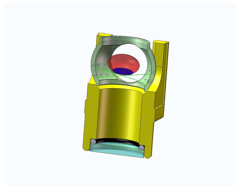
Figure 1a. Figure shows a section view of the immersion cell. The immersion cell contains a supporting mesh made of 10-0 nylon sutures on which lenses of various sizes can be placed for shadow-photogrammetry.

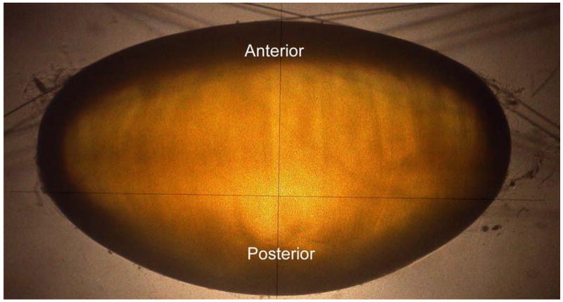
Figure 1b. Shadow-photogrammetric images of a human crystalline lens. The lens is supported on a mesh made of 10-0 nylon sutures (10 μm diameter), enabling both sides of the lens to be available for contour detection.

Shadow-photogrammetry

The technique of shadow-photogrammetry of eye tissues has been described in detail in earlier publications (Denham, Holland, Mandelbaum, Pflugfelder and Parel, 1989; Pflugfelder, Roussel, Denham, Feuer, Mandelbaum and Parel, 1992; Rosen et al 2006; Augusteyn et al, 2006). In short a modified optical comparator (BP-30S, Topcon, Tokyo, Japan) projects a 20x magnified shadow of an excised lens onto a viewing screen. Two light sources enabled photography of the lens in the coronal and sagittal views. The immersion cell described in Rosen et al (2006) was modified by replacing the lens-holding ring with a supporting mesh made of 10-0 nylon sutures. This enabled the entire posterior surface of the lens to be available for contour detection (Figure 1b). A 4.0 Mp Nikon Coolpix 4500 digital camera (Tokyo, Japan) positioned at a fixed distance from the screen was used to capture the coronal and sagittal views of the lens. A ruler (1376T-25, Keuffel and Esser Co., Hoboken, New Jersey) was also photographed on each image for scaling purposes.

Image Analysis

The images were preprocessed with Canvas 9.0 (ACD Systems of America, Miami, FL). They were scaled against the ruler included in the image and were adjusted for magnification (20x) of the comparator. The images were then cropped to remove the ruler. The preprocessed images were loaded into MATLAB (Mathworks, Inc., Natick MA) and converted to 8-bit grayscale images. An algorithm composed of two separate processes was used to detect the lens-contour. The first process detected a thick approximate contour of the lens, using the Prewitt edge detector and morphological functions. This eliminated false edges generated by the sutures zonules, adherent vitreous and other material extraneous to the lens. The second separate process used the Canny edge detector, to detect a fine contour of the lens. An intersection of the outputs of the two processes produces the lens contour with minimal false contours. A few false contours that were detected were removed manually. For the majority of the images, the size of each pixel in the plane of the lens was between 4 and 5 μm.

The post-processed images were loaded into MATLAB and the pixels corresponding to the lens contour were extracted. The lens was aligned such that the posterior surface of the lens was on top (Figure 2). The midpoint of the outermost pixels at the equator along the X axis was estimated to be the position of the optical axis. The position of the equatorial axis was estimated to be the midpoint of the outermost pixels at the equator, along the Y axis. The center of the lens was estimated to be the point of intersection of the optical axis and the equatorial axis. To correct the contour for tilts, the lens was split in half at the optical axis, and both halves were rotated, until the root mean squared error between the two halves was minimized.

Figure 2.

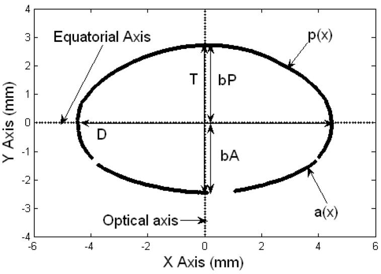
The coordinate system of the Two Curves method. The equatorial axis is parallel to the X axis and the optical axis is parallel to the Y axis. The anterior surface of the lens is positioned in the 3^rd and 4^th quadrants of the co-ordinate system and the posterior surface in the 1^st and 2^nd quadrants. The data set of pixel coordinates above the equatorial axis corresponds to the posterior segment of the lens, and the set below, corresponds to the anterior segment of the lens. The diameter (D), thickness (T), anterior thickness (bA) and posterior thickness (bP) are shown. p(x) is the posterior TCM polynomial and a(x) is the anterior TCM polynomial. Gaps on the lens surface are regions where the edge detection algorithm could not identify the lens profile.

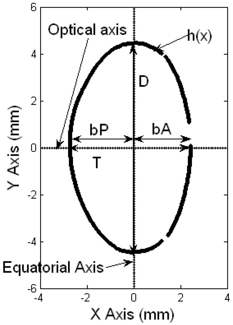
The centered lens contour was analyzed in two ways. In the first method, the Two-Curves Method (TCM) (Figure 2), the lens was divided at the equatorial axis to obtain the anterior and posterior surfaces of the lens. The anterior surface of the lens was positioned in the 3^rd and 4^th quadrants of the co-ordinate system and the posterior surface in the 1^st and 2^nd quadrants. The two surfaces were fit to 10^th-order even polynomials. In the One-Curve Method (OCM) (Figure 3), the anterior surface of the lens was positioned in the 1^st and 4^th quadrants of the coordinate system and the posterior surface in the 2^nd and 3^rd quadrants. The lens was split in half at the optical axis to obtain the contour of one half-meridional section of the lens. This contour was fit to a 10^th-order polynomial. Curve fitting for both methods was performed using the Levenberg-Marquardt algorithm of MATLAB’s curve fitting toolbox. The results were independent of the starting points provided.

Figure 3.

The coordinate system of the One Curve method (OCM). The optical axis is parallel to the X axis and the equatorial axis is parallel to the Y axis. The anterior surface of the lens is positioned in the 1^st and 4^th quadrants of the coordinate system and the posterior surface in the 2^nd and 3^rd quadrants. The data set of the pixel coordinates above the optical axis was used in this method. The diameter (D), thickness (T), anterior thickness (bA) and posterior thickness (bP) are shown. h(x) is the OCM polynomial. Gaps on the lens surface are regions where the edge detection algorithm could not identify the lens profile.

In the TCM, the equatorial diameter (D) was estimated as the distance between the points of intersection of the two polynomials representing the anterior and posterior surfaces of the lens. The points of intersection of the two polynomials were determined by solving the two equations. The anterior sagittal thickness (bA) and the posterior sagittal thickness (bP) were obtained from the y offsets of the respective fits, and the total sagittal thickness was estimated as the sum of the two. The cross-sectional area (CSA) of the lens was computed by integrating the fits. Assuming rotational symmetry around the optical axis, the anterior and posterior surface area of the lens was estimated by computing the surface of revolution of the anterior and posterior fits around the optical axis. The two surface areas were added to obtain the total surface area of the lens. The volume (V) of the lens was estimated by computing the solid of revolution of the cross-sectional plane around the optical axis. The equations for the polynomials, cross-sectional area (CSA), surface area (SA) and volume (V) for the TCM are listed in Table 1.

Table 1.

Equations of polynomials, cross-sectional area (CSA), surface area (SA) and volume (V) for the Two Curves Method (TCM) and the One Curve Method (OCM). p(x) is the posterior polynomial, a(x) is the anterior polynomial and h(x) is the polynomial representing the contour of a half-meridional section of the lens. The coefficients of the three polynomials are denoted by f_p, f_a and f_h. D, bA and bP are the diameter, anterior thickness and posterior thickness of the lens.

Two Curves Method (TCM)	One Curve Method (OCM)
$p(x)=bP+{\displaystyle \sum _{i=1}^5}{f}_{p(2i)}{(x)}^{2i}$	$h(x)=\frac{D}{2}+{\displaystyle \sum _{i=1}^{10}}{f}_{h(i)}{(x)}^i$
$a(x)=-bA+{\displaystyle \sum _{i=1}^5}{f}_{a(2i)}{(x)}^{2i}$
$\mathit{CSA}={\displaystyle \underset{-D/2}{\overset{D/2}{\int }}}[p(x)-a(x)]dx$	$\mathit{CSA}=2{\displaystyle \underset{-bP}{\overset{bA}{\int }}}h(x)dx$
$\begin{array}{l}SA=2\pi {\displaystyle \underset{0}{\overset{D/2}{\int }}}x\sqrt{1+{\left[p^{\prime }(x)\right]}^2}dx\\ +2\pi {\displaystyle \underset{0}{\overset{D/2}{\int }}}x\sqrt{1+{\left[a^{\prime }(x)\right]}^2}dx\end{array}$	$SA=2\pi {\displaystyle \underset{-bP}{\overset{bA}{\int }}}h(x)\sqrt{1+{[h^{\prime }(x)]}^2}dx$
$V=2\pi {\displaystyle \underset{0}{\overset{D/2}{\int }}}x[p(x)-a(x)]dx$	$V=\pi {\displaystyle \underset{-bP}{\overset{bA}{\int }}}{[h(x)]}^{2}dx$

In the OCM, the anterior sagittal thickness (bA) and the posterior sagittal thickness (bP) were obtained by the solving the OCM equation for y=0. The two thicknesses were added to obtain the total sagittal thickness. Diameter (D) was estimated as twice the y offset of the fit. The cross-sectional area (CSA) of the lens was estimated as twice the area under the curve. Assuming rotational symmetry, the surface area (SA) of the lens was estimated by computing the surface of revolution of the fitted curve around the optical axis and the volume (V) of the lens was estimated by computing the solid of revolution of the cross-sectional plane around the optical axis. The equations for the polynomial, cross-sectional area (CSA), surface area (SA) and volume (V) for the OCM are listed in Table 1.

Data Analysis

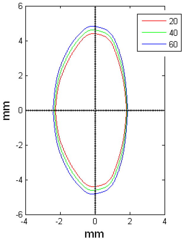
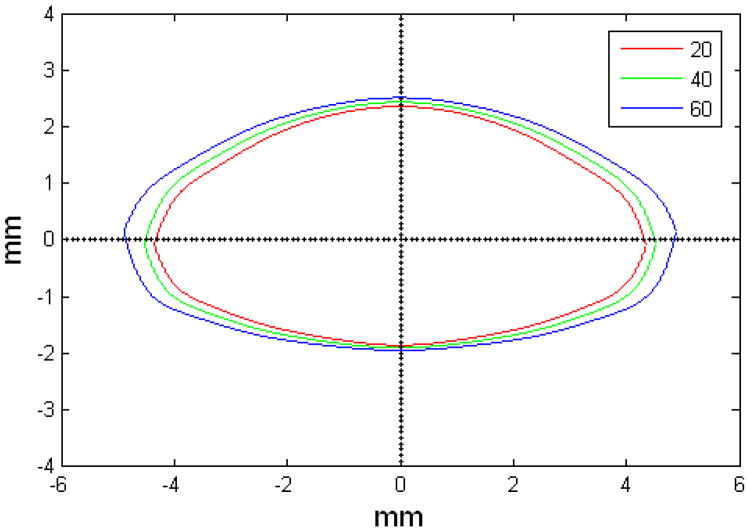
The diameter (D), thickness (T), anterior thickness (bA), posterior thickness (bP), cross-sectional area (CSA), surface area (SA) and volume (V) obtained from the two methods were analyzed as a function of age using linear regressions (Table 2 and Figures 4–6). The coefficients of the polynomials for each of the three curves were analyzed as a function of age (Table 3 and Figures 7 and 8). Using these coefficients, the lens shapes for 20, 40 and 60 year old lenses were plotted. The top half of the OCM model was plotted after solving the equation for y=0. The bottom half was obtained by reflecting the curve at the X axis (Figure 9). The TCM model was plotted up to the points of intersection of the anterior and posterior curves (Figure 10). For each of the methods the dimensions used (D, bA and bP), were obtained from the linear regressions of the method itself.

Table 2.

Dimensions of the crystalline lens obtained from the One Curve Method (OCM) and the Two Curves methods (TCM) (n=27) compared to dimensions measured from images manually in Rosen et al.

Dimension	One Curve Method	Two Curves Method	Rosen et al
Diameter (D) [mm]	8.38 (±0.22) + 0.021 (±0.004) × Age (R2=0.48; p<0.0001)	8.47 (±0.23) + 0.022 (±0.005) × Age (R2=0.45; p<0.0001)	8.7 (±0.14)+ 0.014 (±0.002) × Age (R2=0.57; p<0.0001)
Thickness (T) [mm]	4.11 (±0.16) + 0.006 (±0.003) × Age (R2=0.13; p=0.060)	4.1 (±0.16) + 0.006 (±0.003) × Age (R2=0.13; p=0.066)	3.97 (±0.16)+ 0.013 (±0.003) × Age (R2=0.48; p<0.0001)
Anterior Thickness (bA) [mm]	1.82 (±0.1) + 0.002 (±0.002) × Age (R2=0.05; p=0.2296)	1.82 (±0.1) + 0.002 (±0.002) × Age (R2=0.05; p=0.26819)	1.65 (±0.075)+ 0.005 (±0.001) × Age (R2=0.45; p<0.0001)
Posterior Thickness (bP) [mm]	2.29(±0.12) + 0.004 (±0.002) × Age (R2=0.1; p=0. 0.116)	2.28(±0.12) + 0.004 (±0.002) × Age (R2=0.1; p=0. 0.116)	2.33 (±0.11)+ 0.007 (±0.002) × Age (R2=0.44; p<0.0001)

Figure 4.

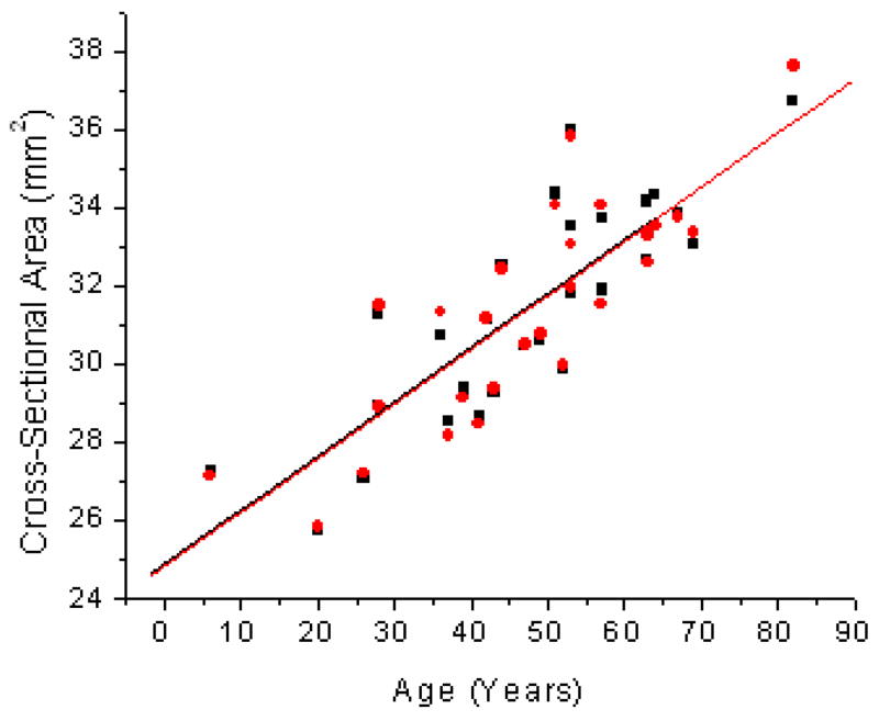
Age related changes in Cross-Sectional Area (CSA) of the human lens for the One Curve Method (OCM; ●) and the Two Curves Method (TCM; ■). Linear fits of the data indicated CSA = 24.8 (±0.9) + 0.14 (±0.02) × Age (R²=0.69; p<0.0001) for OCM and CSA = 24.9 (±0.9) + 0.14 (±0.02) × Age (R²=0.69; p<0.0001) for TCM.

Figure 6.

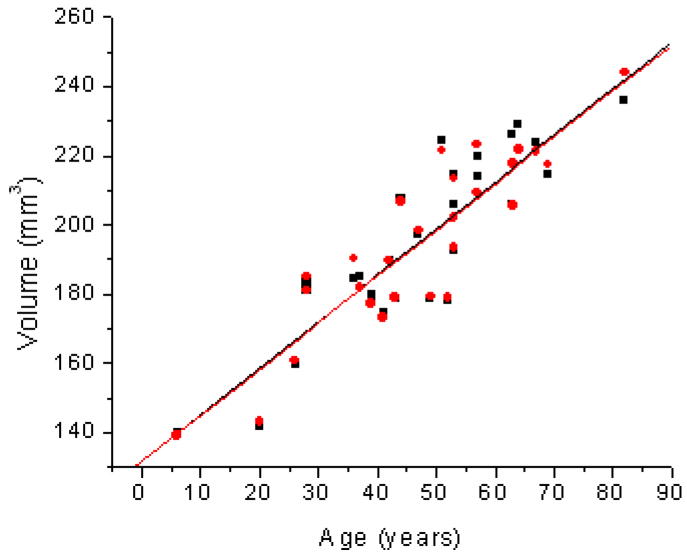
Age related changes in Volume (V) of the human lens for the One Curve Method (OCM; ●) and the Two Curves Method (TCM; ■). Linear fits of the data indicated V = 131.6 (±7.0) + 1.35 (±0.14) × Age (R²=0.78; p<0.0001) for OCM and V = 131.6 (±7.0) + 1.35(±0.14) × Age (R²=0.78; p<0.0001) for TCM.

Table 3.

Coefficients of 10^th-order polynomials representing half curve (f_hxx), anterior segment (f_axx) and posterior segment (f_pxx) of the lens, where f_·xx = A + B × Age (n=27). Coefficients that showed a significant trend with age (p<0.1) are marked with an asterisk (*). The root mean squared errors (rmse) for the curve-fits ranged from 11 to 70 μm for the OCM, 8 to 134 μm for the anterior surface of the TCM and 9 to 27 μm for the posterior surface of the TCM.

Polynomial Coefficient	A	% variability of A	B	% variability of B	R2	p value
One Curve Method
fh01	−0.073± 0.087	119	−0.0010± 0.0017	165	0.01	0.55
fh02	−0.531± 0.173	33	9.997E-4± 0.005	348	0.003	0.78
fh03	0.641± 0.199	31	−2.268E-4± 0.004	1764	1.3E-4	0.95
fh04	−0.118± 0.324	274	0.0021± 0.0065	312	0.004	0.75
fh05	−0.840± 0.243	28	0.0023± 0.0049	215	0.01	0.65
fh06	−0.160± 0.179	112	1.807E-4± 0.0036	1992	1.0E-4	0.96
fh07	0.351± 0.114	33	−0.0013± 0.0023	176	0.01	0.57
fh08	0.111± 0.041	38	−5.507E-4± 8.335E-4	151	0.02	0.51
fh09	−0.052± 0.019	37	2.157E-4± 3.829E-4	177	0.01	0.58
fh10	−0.020± 0.005	27	1.100E-4± 1.067E-4	97	0.13	0.31
Two Curve Method – Anterior Surface
fa02*	0.115± 0.015	13	−8.707E-4± 3.015E-4	35	0.25	0.08
fa04	−0.019± 0.005	26	1.679E-4± 1.016E-4	60	0.10	0.11
fa06*	0.003± 7.17E-4	23	−2.934E-5± 1.440E-5	49	0.14	0.05
fa08*	−2.326E-4± 4.486E-5	19	2.389E-6±9.009E-7	37	0.22	0.01
fa10*	6.256E-6±1.063E-6	17	−7.090E-8± 2.134E-8	30	0.31	0.003
Two Curves Method – Posterior Surface
fp02	−0.119± 0.012	10	3.689E-4± 2.330E-4	63	0.09	0.13
fp04	0.007± 0.004	51	4.993E-6± 7.422E-5	1486	1.8E-4	0.95
fp06	−0.002± 6.274E-4	32	1.468E-5± 1.260E-5	85	0.05	0.25
fp08*	1.911E-4± 4.610E-5	24	−2.093E-6± 9.259E-7	44	0.17	0.03
fp10*	−5.881E-6± 1.248E-6	21	7.519E-8± 2.507E-8	33	0.51	0.006

Figure 7.

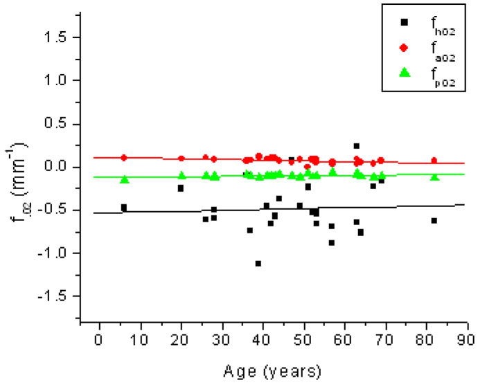
Age related changes in the 2^nd-order coefficient of the OCM curve (f_h02; ■), the anterior curve of the TCM (f_a02; ●) and the posterior curve of the TCM (f_p02; ▲). Linear fits of the data indicated f_h02 = −0.53 (±0.17) + 9.9E-4 (±3.48E-3) × Age (R²=0.003; p=0.78), f_a02 = 0.11 (± 0.02) + −8.7E-4 (± 3.0E-4) × Age (R²=0.25; p=0.008) and f_p02 = −0.12 (± 0.01) + 3.7E-4 (± 2.3E-4) × Age (R²=0.09; p=0.13).

Figure 8.

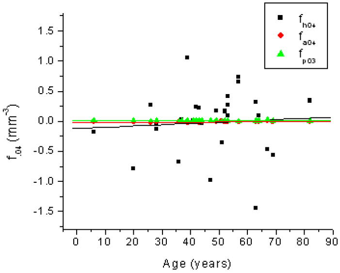
Age related changes in the 4^th-order coefficient of the OCM curve (f_h04; ■), the anterior curve of the TCM (f_a04; ●) and the posterior curve of the TCM (f_p04; ▲). Linear fits of the data indicated f_h04 = −0.118 (± 0.32) + 0.002 (± 0.006) × Age (R²=0.004; p=0.75), f_a04 = −0.019 (± 0.005) + 1.68E-4 (± 1.02E-4) × Age (R²=0.1; p=0.11) and f_p04 = 0.0072 (± 0.004)+ 4.99E-6 (± 7.42E-5) × Age (R²=1.8E-4; p=0.95).

Figure 9.

OCM model of 20 (red), 40 (green) and 60 (blue) year old lenses.

Figure 10.

TCM model of 20 (red), 40 (green) and 60 (blue) year old lenses.

3. Results

Table 2 shows that all dimensions increase as the lens ages from ages 6 to 82 years. Figures 4–6 show the linear regressions of the cross-sectional area, surface area and volume of the lens with age. All three quantities exhibited statistically significant increasing trends (p<0.0001).

Table 3 shows the linear regression equations of the polynomial coefficients with age. The root mean squared errors (rmse) for the polynomial fits ranged from 11 to 70 μm for the OCM, 8 to 134 μm for the anterior surface of the TCM and 9 to 27 μm for the posterior surface of the TCM. The coefficients of the OCM did not display a significant trend with age. The 2^nd, 6^th and 10^th-order coefficients of the anterior surface of the TCM decreased with age while the 8^th-order coefficient increased. For the posterior surface of the TCM, the 8^th-order coefficient significantly decreased with age and the 10^th-order coefficient increased. The coefficient of all other terms of the anterior and posterior surfaces of the TCM did not change significantly with age. Figures 7 and 8 show the age dependency of the 2^nd-order and 4^th-order coefficients of the three curves. All coefficients displayed a high percentage of uncertainty. The uncertainty of the coefficients that displayed a statistically significant trend with age (p<0.1) ranged from 30% to 49%.

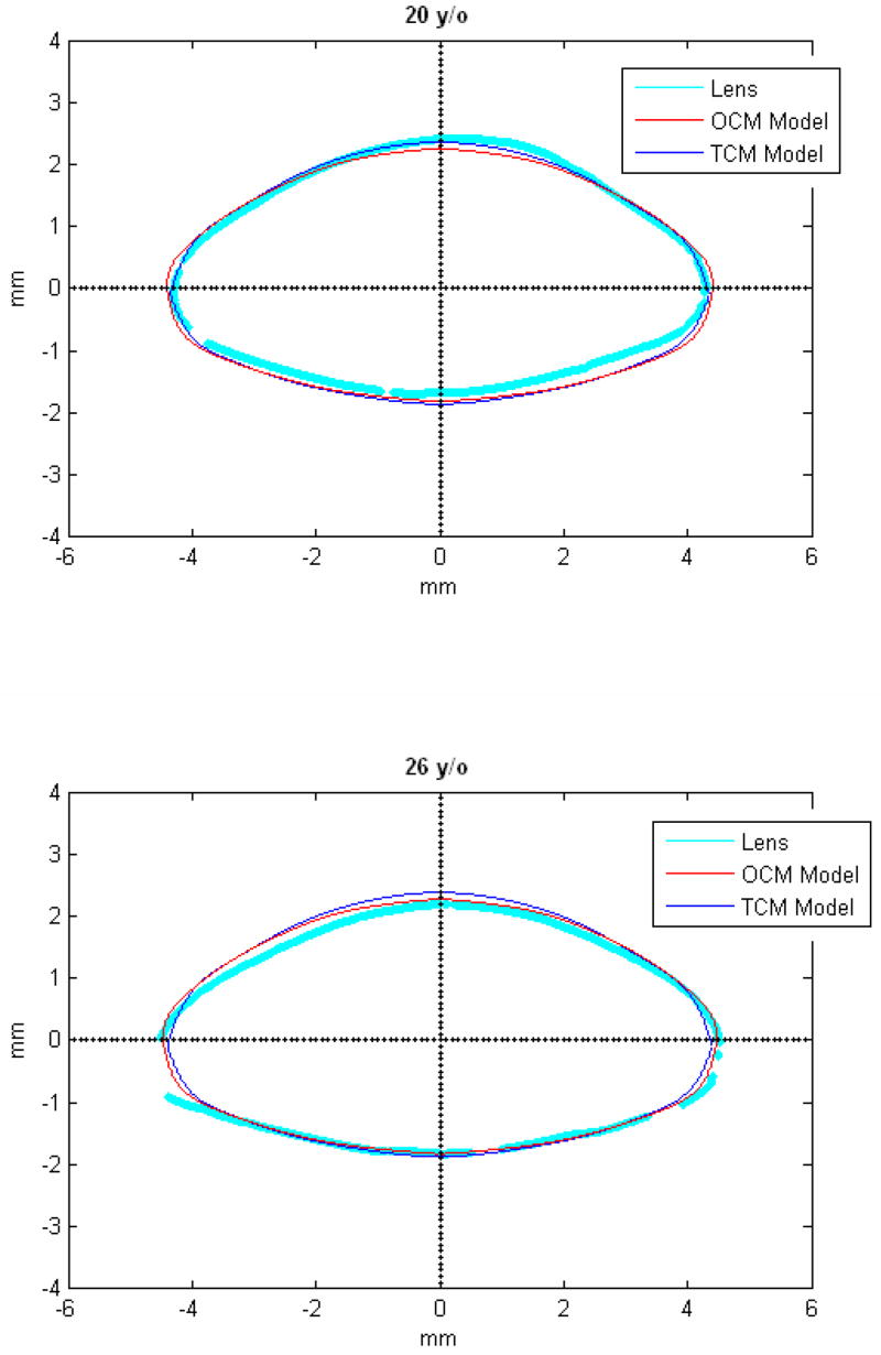
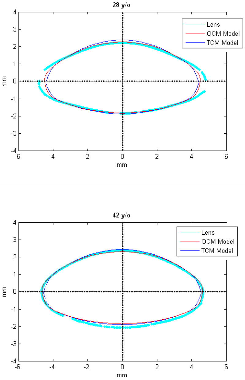
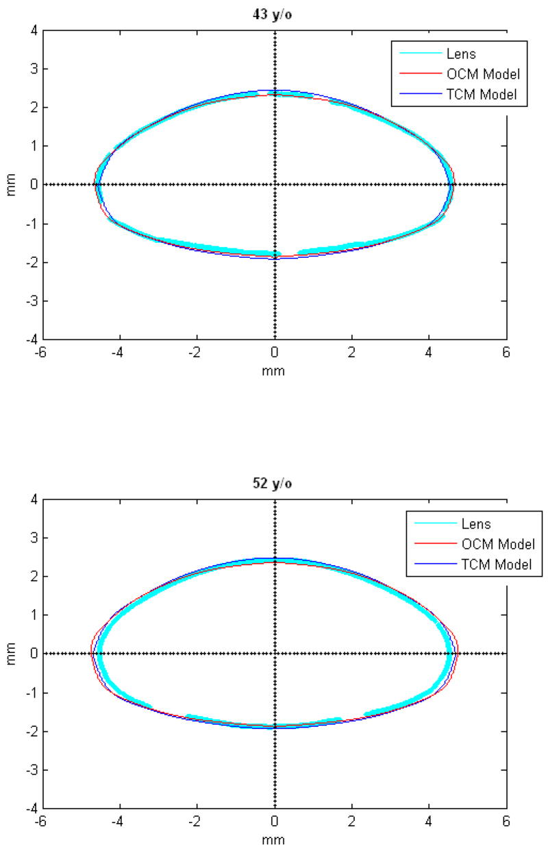
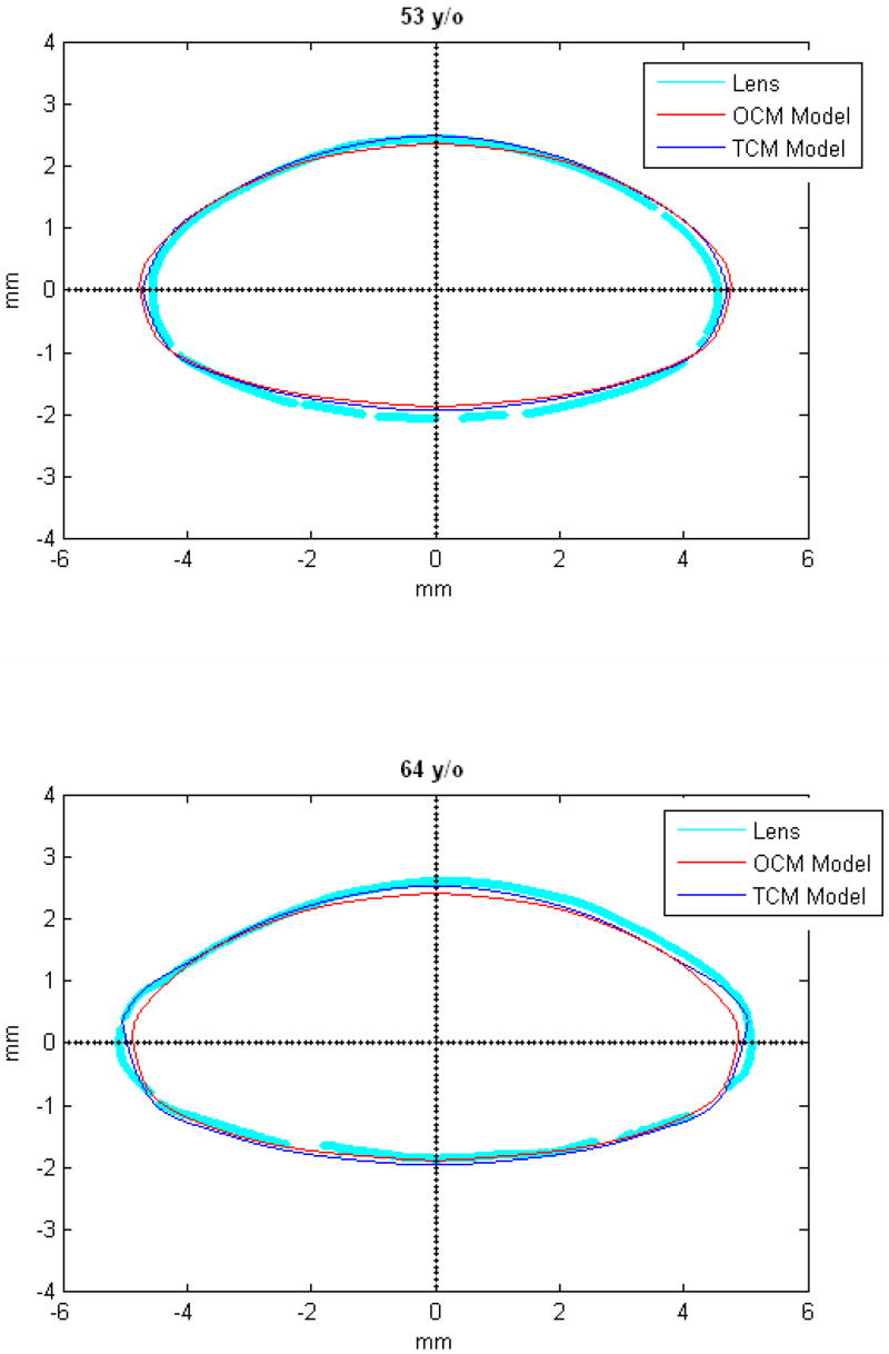
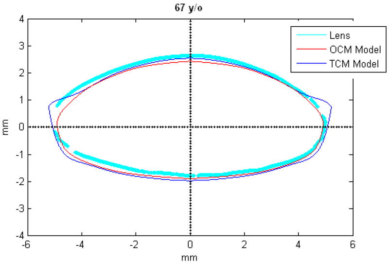
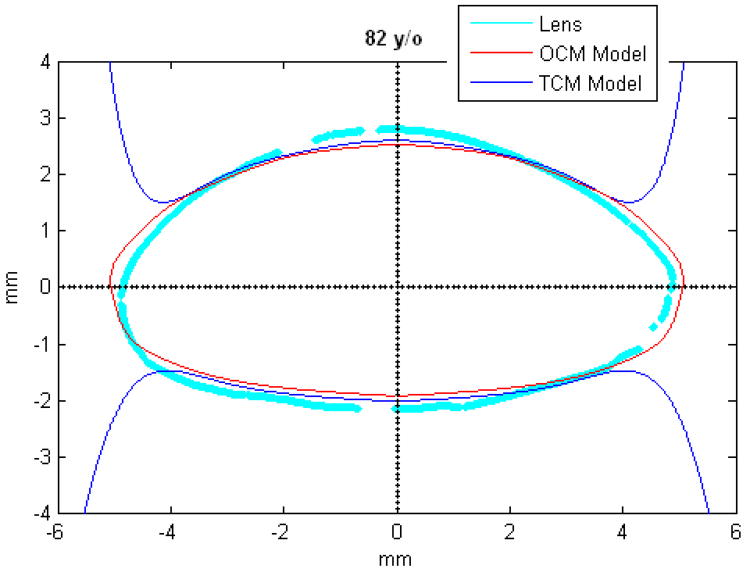
Figures 9 and 10 show the OCM and TCM models for lenses aged 20, 40 and 60 years. Supplementary movies 1 and 2 show the growth of the lens as predicted by the two models from ages 20 to 82 years for the OCM and from 20 to 60 years for the TCM. Both models were superimposed on lens profiles of various ages (Figure 11).

Figure 11.

TCM (blue) and OCM (red) models superimposed on the profile of lenses (cyan) of various ages. The TCM and the OCM models were plotted with coefficients obtained via linear regression presented in Table 3. The differences between the models and the lens profiles are due to variability of individual lenses.

4. Discussion

In this study, shadow-photogrammetric images of freshly isolated ex-vivo human crystalline lenses were analyzed to obtain age-dependent models through linear regression of the coefficients of the polynomial fits. Shadow-photogrammetric images have a pixel size of 4–5 μm and have good contrast enabling exceptional contour detection. These two factors improve the accuracy of the fits. Shadow-photogrammetry is based on precision optical comparator technology and employs a telecentric light beam, which introduces no distortions to the lens surface. Therefore, unlike OCT (Optical Coherence Tomography) or Scheimpflug images, these images do not need correction to the shape of the lens. With shadow-photogrammetry, lenses with capsular defects such as separations and cataracts can be identified and therefore be excluded from analysis. The limitation of shadow-photogrammetry is that it cannot be used on in-vivo lenses. The placement of the ex-vivo lens in the immersion cell may introduce a slight tilt in the sagittal plane.

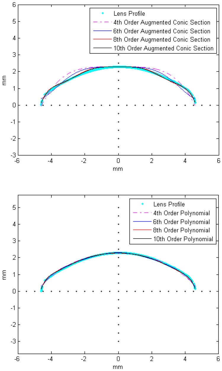
The lenses were analyzed with two methods, the OCM, where half the contour of the lens was modeled and the TCM, where the contours of the anterior and posterior surfaces were analyzed separately. Symmetry around the optical axis was assumed for both methods. The two surfaces of the TCM method were fit to 10^th-order even polynomials, while the surface from the OCM was fit to 10^th-order polynomials. Polynomials were chosen because a single higher order augmented conic function similar to that which was used by Rosen et al (2006) did not provide a good fit around the equatorial regions (Figures 12-a and 12-b). It is feasible to fit the lens surface to age-dependent piecewise continuous conic sections or other piecewise continuous functions, but this approach would significantly increase the complexity of the age-dependent model.

Figure 12. Illustrative example of a posterior lens surface (cyan) fit with augmented conic sections.

(a) and even polynomials (b). RMSE of the fits were 223 μm, 138 μm, 62 μm, 53 μm for the 4^th, 6^th, 8^th and 10^th order conic sections and 50 μm, 40 μm, 39 μm and 32 μm for the 4^th, 6^th, 8^th and 10^th order polynomials respectively.

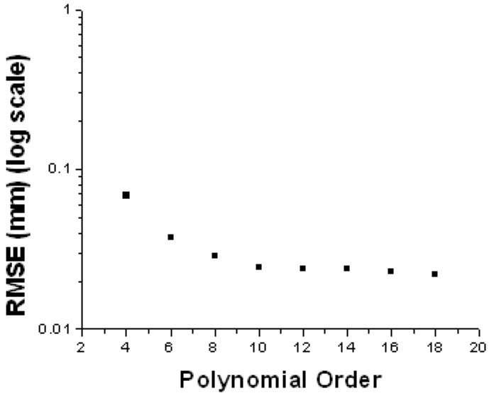
In a preliminary analysis polynomials of several orders were fit to lens surfaces. 10^th-order polynomials were chosen because the rmse of the fits converged at order 10 and did not decrease significantly for orders higher than 10 up to order 18 (Figure 13).

Figure 13. Illustrative example of the effect of the polynomial order on the RMSE fit of a posterior lens surface.

Overall, RMSE values converged at order 10 and did not decrease significantly for orders higher than 10.

Polynomials serve as good mathematical models to describe the whole shape of the lens and for biometric computations. The advantage of using polynomials is that they capture the age-dependence of the whole lens shape in one or two equations. However, polynomials have inherent problems, which make them less optimal for direct use in optical and mechanical modeling. The derivatives are discontinuous at the apexes for the OCM and at the equatorial plane for the TCM. The second derivatives (i.e. curvature) of both models vary strongly along the profile.

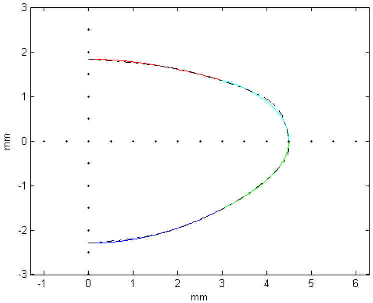
These problems can be circumvented by using the polynomials as a basis to fit functions with any specific properties as required for FE modeling or any other application. As an example we fit conic sections such as those used by Hermans et al (2006) to the 29-year-old OCM lens (Figure 14). The central 6 mm was fit to conic sections and the periphery was modeled by two more conic sections whose first derivatives were set to be continuous with the central conics. The functions fit closely to the OCM model. The central radii of curvature (8.03 mm for the anterior surface and −6 mm for the posterior surface) were comparable to published values (Borja et al 2008). Another approach would be to combine the TCM and the OCM models to obtain continuous first derivatives along the profile of the lens. The central region of the lens could be modeled with the TCM and the equatorial region with the OCM.

Figure 14.

The central 6 mm of the 29-year-old OCM lens (dashed line) was fit to conic sections (red and blue) similar to those used by Hermans et al (2006). The equatorial region was modeled with two conic functions (green and cyan) whose derivatives were set to be continuous with the central conics. The radii of curvature obtained with these fits were 8.03 mm for the anterior surface and −r the posterior surface.

The advantages of fitting to the OCM and TCM models are that they are age dependent and are based on measurements of ex-vivo lenses. The isolated ex-vivo lens is not subject to any active forces and its shape would be comparable to the shape of the maximally accommodated in-vivo lens (Dubbelman et al 2005, Rosen et al 2006). The starting point of FE models should be one where no forces are applied. Therefore new FE models can be developed for any age using the presented polynomial models.

The diameter of the lens estimated by the two models (Table 2) was lower, and the thickness of the lens was higher than the manual measurements reported in an earlier study (Rosen et al 2006). However, the three datasets became comparable after the 6-year-old lens was excluded. This difference indicates that young lenses do not follow a linear growth pattern (Augusteyn 2007). Augusteyn (2007) showed that the lens growth occurs in two phases, an initial mode of rapid growth during pre-natal development and a second, linear growth mode, throughout life. A reduction in lens thickness has been reported up to the age of 10 to 13 years (Zadnik, Mutti, Fusaro & Adams 1995;Mutti, Zadnik, Fusaro, Friedman, Sholtz, & Adams 1998; Augusteyn 2008). Here, a linear fit was chosen for the dimensions because of the limited number of young lenses available. More young lenses are required to show the non-linear age dependence of lens growth.

Lens cross-sectional areas (CSA) obtained from both methods range from 26 to 37 mm² (Figure 4). For the age range of 20 to 55 years, Strenk et al (2004) reported a CSA range of 22 to 30 mm² for the accommodated eye, in-vivo, using MRI images. Examination of data from Glasser and Campbell (1999) for this age range, for the in-vitro lens, revealed a CSA range of 18 to 23 mm². The difference in measurements could be due to the different mathematical models that were used to represent the lens surfaces. Strenk et al (2004) used 4^th-order polynomials to model the lens surfaces, while Glasser and Campbell (1999) used second order polynomials.

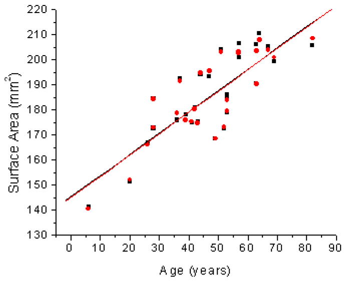
The surface area (SA) of the lens (Figure 6) increases with age, indicating that there is an increased tension in the lens capsule as the lens ages. The range of surface areas obtained was 150 to 215 mm² from both the OCM and the TCM. Total lens surface areas have only been reported by Hermans et al (2007), who predicted surface area using FE models whose geometry was based on information from Scheimpflug images. They reported surface areas of 141 to 166 mm² for lenses aged 11, 29 and 45 years. For this age range, the surface area was 154 to 183 mm² as predicted by the OCM and was 155 to 184 mm² as predicted by the TCM. These values are comparable.

The main goal of this study was to develop an age-dependent mathematical model to describe the shape of the whole ex-vivo human crystalline lens. This model should provide an uncomplicated and accurate calculation technique for lens biometry and also serve as a foundation for developing suitable models for computational modeling, especially for FE modeling. This was achieved by using the linear regression of the coefficients of the polynomial fits. To verify that the equations can be used, shapes of 20, 40 and 60 year old lenses were plotted for the OCM (Figure 9) and the TCM models (Figure 10). The two models were also superimposed on lens profiles of various ages (Figure 11). Both models provide a close estimate of the shape of the lens, however, figures 11-i and 11-j show that with the TCM model, the lens shape is reliably modeled from age 20 to 60 years only. Beyond that the TCM modeled shape is inconsistent with the shape of the lens.

Both methods described in this paper can be used to obtain dimensions of the human crystalline lens. Both of the age-dependent models can be used to model the shape of the lens from ages 20 to 60 years, but only the OCM model can be used for older lenses. Another advantage of the OCM model is that it describes the lens with only one mathematical equation making it a simple model. The two age-dependent models of the isolated ex-vivo human crystalline lens, presented above, can, with additional processing, serve to improve FE-models of lenses.

Figure 5.

Age related changes in Surface Area (SA) of the human lens for the One Curve Method (OCM; ●) and the Two Curves Method (TCM; ■). Linear fits of the data indicated SA = 145.0 (±5.8) + 0.85 (±0.11) × Age (R²=0.68; p<0.0001) for OCM and SA = 145.2 (±6.0) + 0.8 (±0.1) × Age (R²=0.67; p<0.0001) for TCM.

References

- Abolmaali A, Schachar RA, Le T. Sensitivity study of human crystalline lens accommodation. Computer methods and programs in biomedicine. 2007;85:77–90. doi: 10.1016/j.cmpb.2006.08.005. [DOI] [PubMed] [Google Scholar]
- Augusteyn RC, Rosen AM, Borja D, Ziebarth NM, Parel JM. Biometry of primate lenses during immersion in preservation media. Molecular Vision. 2006;12:740–747. [PubMed] [Google Scholar]
- Augusteyn RC. Growth of the human eye lens. Molecular Vision. 2007;13:252–257. [PMC free article] [PubMed] [Google Scholar]
- Augusteyn RC. Growth of the lens: in vitro observations. Clin Exp Optom. 2008;91:226–239. doi: 10.1111/j.1444-0938.2008.00255.x. [DOI] [PubMed] [Google Scholar]
- Borja D, Manns F, Ho A, Ziebarth NM, Rosen AM, Jain R, Amelinckx A, Arrieta E, Augusteyn RC, Parel JM. Optical power of the isolated human crystalline lens. Invest Ophthalmol Vis Sci. 2008;49:2541–2548. doi: 10.1167/iovs.07-1385. [DOI] [PMC free article] [PubMed] [Google Scholar]
- Brown N. The change in shape and internal form of the lens of the eye on accommodation. Experimental eye research. 1973;15:441–459. doi: 10.1016/0014-4835(73)90136-x. [DOI] [PubMed] [Google Scholar]
- Burd HJ, Judge SJ, Flavell MJ. Mechanics of accommodation of the human eye. Vision Research. 1999;39:1591–1595. doi: 10.1016/s0042-6989(98)00298-3. [DOI] [PubMed] [Google Scholar]
- Burd HJ, Judge SJ, Cross JA. Numerical modelling of the accommodating lens. Vision Research. 2002;42:2235–2251. doi: 10.1016/s0042-6989(02)00094-9. [DOI] [PubMed] [Google Scholar]
- Denham D, Holland S, Mandelbaum S, Pflugfelder S, Parel JM. Shadow photogrammetric apparatus for the quantitative evaluation of corneal buttons. Ophthalmic Surgery. 1989;20:794–799. [PubMed] [Google Scholar]
- Dubbelman M, van der Heijde GL. The shape of the aging human lens: curvature, equivalent refractive index and the lens paradox. Vision Research. 2001;41:1867–1877. doi: 10.1016/s0042-6989(01)00057-8. [DOI] [PubMed] [Google Scholar]
- Dubbelman M, van der Heijde GL, Weeber HA. Change in shape of the aging human lens with accomodation. Vision Research. 2005;45:117–132. doi: 10.1016/j.visres.2004.07.032. [DOI] [PubMed] [Google Scholar]
- Glasser A, Campbell MC. Biometric, optical and physical changes in the isolated human crystalline lens with age in relation to presbyopia. Vision Research. 1999;39:1991–2015. doi: 10.1016/s0042-6989(98)00283-1. [DOI] [PubMed] [Google Scholar]
- Hermans EA, Dubbelman M, van der Heijde GL, Heethaar RM. Estimating the external force acting on the human eye lens during accommodation by finite element modelling. Vision Research. 2006;46:3642–3650. doi: 10.1016/j.visres.2006.04.012. [DOI] [PubMed] [Google Scholar]
- Hermans EA, Dubbelman M, van der Heijde GL, Heethaar RM. Change in the accommodative force on the lens of the human eye with age. Vision Research. 2008;48:119–126. doi: 10.1016/j.visres.2007.10.017. [DOI] [PubMed] [Google Scholar]
- Howcroft MJ, Parker JA. Aspheric curvatures for the human lens. Vision Research. 1977;17:1217–1223. doi: 10.1016/0042-6989(77)90157-2. [DOI] [PubMed] [Google Scholar]
- Kasprzak HT. New approximation for the whole profile of the human crystalline lens. Ophthalmic Physiol Opt. 2000;20:31–43. [PubMed] [Google Scholar]
- Koretz JF, Handelman GH. Model of the accommodative mechanism in the human eye. Vision Research. 1982;22:917–927. doi: 10.1016/0042-6989(82)90028-1. [DOI] [PubMed] [Google Scholar]
- Koretz JF, Handelman GH. A model for accommodation in the young human eye: The effects of lens elastic anisotropy on the mechanism. Vision Research. 1983;23:1679–1686. doi: 10.1016/0042-6989(83)90183-9. [DOI] [PubMed] [Google Scholar]
- Koretz JF, Handelman GH, Brown N. Analysis of human crystalline lens curvature as a function of accommodative state and age. Vision Research. 1984;24:1141–1151. doi: 10.1016/0042-6989(84)90168-8. [DOI] [PubMed] [Google Scholar]
- Krueger RR. Retinal imaging aberrometry, author reply. Ophthalmology. 2002;109:406–407. doi: 10.1016/s0161-6420(01)00918-6. [DOI] [PubMed] [Google Scholar]
- Lizak MJ, Datiles MB, Aletras AH, Kador PF, Balaban RS. MRI of the human eye using magnetization transfer contrast enhancement. Invest Ophthalmol Vis Sci. 2000;41:3878–3881. [PubMed] [Google Scholar]
- Manns F, Fernandez V, Zipper S, Sandadi S, Hamaoui M, Ho A, Parel JM. Radius of curvature and asphericity of the anterior and posterior surface of human cadaver crystalline lenses. Exp Eye Res. 2004;78:39–51. doi: 10.1016/j.exer.2003.09.025. [DOI] [PubMed] [Google Scholar]
- Martin H, Guthoff R, Terwee T, Schmitz KP. Comparison of the accommodation theories of Coleman and of Helmholtz by finite element simulations. Vision Research. 2005;45:2910–2915. doi: 10.1016/j.visres.2005.05.030. [DOI] [PubMed] [Google Scholar]
- Mutti DO, Zadnik K, Fusaro RE, Friedman NE, Sholtz RI, Adams AJ. Optical and structural development of the crystalline lens in childhood. Invest Ophthalmol Vis Sci. 199;39:120–133. [PubMed] [Google Scholar]
- Pflugfelder SC, Roussel TJ, Denham DB, Feuer W, Mandelbaum S, Parel JM. Photogrammetric analysis of corneal trephination. Archives of Ophthalmology. 1992;110:1160–1166. doi: 10.1001/archopht.1992.01080200140042. [DOI] [PubMed] [Google Scholar]
- Rosen AM, Denham DB, Fernandez V, Borja D, Ho A, Manns F, Parel JM, Augusteyn RC. In vitro dimensions and curvatures of human lenses. Vision Research. 2006;46:1002–1009. doi: 10.1016/j.visres.2005.10.019. [DOI] [PubMed] [Google Scholar]
- Strenk SA, Semmlow JL, Strenk LM, Munoz P, Gronlund-Jacob J, DeMarco JK. Age-related changes in human ciliary muscle and lens: a magnetic resonance imaging study. Invest Ophthalmol Vis Sci. 1999;40:1162–1169. [PubMed] [Google Scholar]
- Strenk SA, Strenk LM, Semmlow JL, DeMarco JK. Magnetic resonance imaging study of the effects of age and accommodation on the human lens cross-sectional area. Invest Ophthalmol Vis Sci. 2004;45:539–45. doi: 10.1167/iovs.03-0092. [DOI] [PubMed] [Google Scholar]
- Weeber HA, van der Heijde GL. On the relationship between lens stiffness and accommodative amplitude. Experimental eye research. 2007;85:602–607. doi: 10.1016/j.exer.2007.07.012. [DOI] [PubMed] [Google Scholar]
- Zadnik K, Mutti DO, Fusaro RE, Adams AJ. Longitudinal evidence of crystalline lens thinning in children. Invest Ophthalmol Vis Sci. 1995;36:1581–15877. [PubMed] [Google Scholar]
Associated Data
This section collects any data citations, data availability statements, or supplementary materials included in this article.