Implications of Clinical Trial Design on Sample Size Requirements

Abstract

The primary goal in designing a randomized controlled clinical trial (RCT) is to minimize bias in the estimate of treatment effect. Randomized group assignment, double-blinded assessments, and control or comparison groups reduce the risk of bias. The design must also provide sufficient statistical power to detect a clinically meaningful treatment effect and maintain a nominal level of type I error. An attempt to integrate neurocognitive science into an RCT poses additional challenges. Two particularly relevant aspects of such a design often receive insufficient attention in an RCT. Multiple outcomes inflate type I error, and an unreliable assessment process introduces bias and reduces statistical power. Here we describe how both unreliability and multiple outcomes can increase the study costs and duration and reduce the feasibility of the study. The objective of this article is to consider strategies that overcome the problems of unreliability and multiplicity.

Introduction

The primary goal in designing a randomized controlled clinical trial (RCT) is to minimize bias in the estimate of treatment effects.¹ It is that estimate that reveals whether the treatment is efficacious and, if so, what the magnitude of the effect is. At the same time, an RCT design must seek to achieve other objectives. The study should maintain a nominal level of type I error and provide statistical power that is sufficient to detect a clinically meaningful treatment effect. The RCT must also be both feasible and applicable. That is, the sample size requirements should be truly attainable in the proposed clinical sites, and the burden of the protocol on the participants and investigators cannot be unreasonable. The characteristics of the study sample, based on the inclusion and exclusion criteria, should reflect those of the patient population for whom an indication for the investigational treatment is being sought.

There are 3 fundamental features of RCT design that reduce the risk of bias: randomized group assignment, double-blinded assessments, and control or comparison groups. These sine quo non elements are standard for RCTs in psychopharmacology and are applicable regardless of whether the outcomes focus on clinical symptoms or cognitive function. However, 2 other aspects of RCT design, unreliability and multiplicity, do not necessarily receive sufficient attention. As a result, they are impediments in clinical trial implementation. Multiplicity, comparing the investigational and comparator groups on multiple outcomes, inflates type I error. Unreliability, on the other hand, introduces bias, reduces statistical power and, thus, diminishes the feasibility of a clinical trial. Many task paradigms derived from cognitive neuroscience have either unknown reliability or levels of reliability that may be less than optimal. Further, many such paradigms are complex and may provide several different outcome measures that could be considered equally valid indicators of cognitive improvement. Thus, the problems of unreliability and multiplicity may be particularly acute for RCTs using such measures. The objective of this article is to consider strategies that overcome the problems of unreliability and multiplicity.

Measurement and Sample Size Requirements

In designing an RCT, the choice of assessment for each outcome is critically important, and for that reason, fundamental aspects of candidate measurement tools must be evaluated. First, is the assessment feasible in the target patient population? Second, can it be administered repeatedly over the course of the trial, and if not, are alternative forms available? Third, when selecting appropriate assessments, both the mode of assessment and intensity of training deserve consideration, yet they are all too often overlooked. This has particular bearing on sample size requirements, which will now be considered in detail. Finally, the number of primary efficacy measures must also be determined. The implications for using multiple outcome measures are discussed below in the section on “Multiplicity and Sample Size Requirements.”

Sample Size Determination

The Ethical Guidelines for Statistical Practice from the Committee on Professional Ethics of the American Statistical Association states, “Avoid the use of excessive or inadequate numbers of research subjects by making informed recommendations for study size.”² It is unethical to enroll more subjects than are needed to answer a research question because unwarranted numbers needlessly expose subjects to the risks of research. Conversely, if too few subjects are enrolled in a study, that design will very likely not answer the research question that has been set forth. As a result, the participation of those subjects very well could be for naught, and again their exposure to risk is unjustifiable.

Informed recommendations for study size are, of course, guided by statistical power analyses. The overarching goal of power analyses is to propose a design that is sufficient to provide adequate statistical power to detect a clinically meaningful intervention effect. Consider the 4 components of power analyses. (1) Type I error is typically set at α = .05, unless there are coprimary outcomes (this issue will be discussed again below in the section on “Multiplicity and Sample Size Requirements”). (2) Statistical power of 0.80 is a common goal, although with sufficient resources, both fiscal and human, power of 0.90 could be a reasonable target. (3) The sample size is most often the quantity that is estimated in statistical power analyses. Nonetheless, in some settings, the ideal sample size is highly constrained by resources. (4) The population effect size (eg, Cohen d for a comparison of 2 groups on a continuous outcome) must be deemed clinically meaningful on the metric chosen, preferably based on a consensus among expert clinicians and researchers. An effect size can be expressed in various forms, depending on the nature of the outcome, whether continuous, binary, ordinal, or survival time. Many of these effect sizes, in turn, can be expressed as the number needed to treat (NNT), which is viewed by many to be more clinically interpretable.³ Given any 3 of these power analysis components, the fourth can be determined.

Power is typically manipulated by altering the sample size. To provide some framing, the sample size (N) required for each of 2 treatment groups (assuming equal cell sizes) to detect various effects with statistical power of 0.80 using a t test with a 2-tailed α level of .05 is N = 393 (small effect: d = 0.20), N = 64 (medium effect: d = 0.50), and N = 26 (large effect: d = 0.80).⁴ More subjects are needed to detect smaller treatment effects. A formula for estimating the number of subjects needed per group for statistical power of 0.80 to detect population effect sizes of other magnitudes with a t test is: N = 16/d².⁵ For example, to detect an effect size of d = 0.40, the number of subjects required is: 16/(0.4²) = 100 subjects per group. (Although the examples used throughout this manuscript involve RCTs with 2 groups, each of the issues described is germane to RCTs with more than 2 groups, as well. Likewise, for simplicity, the examples do not involve repeated measures over time, but instead assume that a pre-post change score will be used.)

An alternative to simply manipulating sample size is to consider reducing unreliability of the outcome measure. It has been shown empirically that more reliable outcomes increase the effect size.⁶ Thus, a smaller sample size is needed to detect that larger effect size. Consider the basis for this phenomenon. Cohen d, the between-group effect size for a t test, expresses group mean differences in SD units: 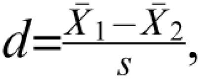where s is the pooled SD. This can be thought of as a signal-to-noise ratio, in which the between-group differences represent the signal and the within-group variability represents noise. If a more reliable assessment procedure is implemented, the response within cell will very likely be less inconsistent. As a result of reducing that noise (ie, the measurement error), the within-treatment group variability will decrease, and this will be reflected in the within-group SDs. Therefore, as unreliability is reduced, the between-group effect size, Cohen d, increases. (This is because the denominator of d comprises within-group variability.) As a consequence, the sample size required for a given level of statistical power decreases with more reliable assessment strategies.

Fleiss stated, “The most elegant design of a clinical study will not overcome the damage caused by unreliable or imprecise measurement.”⁷ Proactive approaches to attenuate this problem involve the selection of a more reliable scale than is typically used, more rigorous rater training, or a novel modality of assessing, perhaps using centralized raters that have already established enhanced reliability.⁸ In the domain of cognitive assessment, increasing the reliability of the outcome measures could be accomplished by (1) increasing the number of trials, (2) improved training and practice approaches, and (3) eliminating sources of noise or variance, such as irrelevant aspects of the tasks. The corresponding reduction in unreliability will reduce the required sample size accordingly. A sample size reduction, in turn, reduces risks to human subjects, reduces RCT study time, and reduces research costs. Therefore, it can be argued that there are ethical implications to the choice of assessment procedure.

We have discussed the virtues of reducing the within-group variability (ie, SD) by attenuating measurement error. Nevertheless, there are components of unreliability that are random noise and might simply increase the variability but remain difficult to eliminate. In addition, there are conditions in which the variability is truncated as a result of undesirable properties of an assessment. For instance, floor and ceiling effects could, in fact, reduce between-group variability, and this runs contrary to the purpose of an RCT. Recent efforts at computer adaptive assessments have sought to stretch the ceiling or floor, based on responses to prior items. Another problem that reduces between-group variability is that of practice effects. Hence, when selecting an assessment process, one must be cognizant of these 3 problems and, if detected, seek to remediate them.

At this point, it is important to diverge somewhat and consider the source for the magnitude of the treatment effect that is used in power analyses. One convention has involved the use of pilot data to guide the choice of effect size. However, Kraemer et al⁹ articulately argue against such a practice and instead state that the objective of a pilot study is to examine the feasibility of the design.⁹ Can subjects be recruited? Will they tolerate the burden of research, including the battery of assessments? Can the treatments be delivered in the proposed manner? In contrast, an effect size from a pilot study is a very imprecise estimate, and it, therefore, poorly informs the sample size determination process. In other words, the confidence interval (CI) around Cohen d, eg, is quite wide when based on the small sample sizes typically seen in pilot studies. Specifically, the 95% CI is estimated as 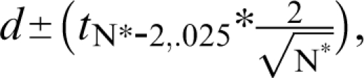where N^* is the total sample size (N^* = 2N). For pilot Ns, the t value will be approximately 2.0. Therefore, a quick approximation for the 95% CI is 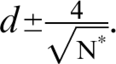For example, with a pilot study sample size of 16 (ie, 8/group) and a sample effect size of the 95% CI for the population effect size ranges from about −0.50 to 1.5. That is, there is a 95% probability that the true population effect size falls some where from superiority of the comparator (by 0.5 SD units) to a tremendous positive effect of the investigational agent (exceeding the comparator by 1.5 SD units). Hence, the estimate from this hypothetical pilot is bathed in imprecision. Other examples, which come from a simulation study, are presented in Figure 1. (Note that Figure 1 displays the N/group, not the total N* used in the preceding example.) The results are based on 10 000 datasets for each N, and these were simulated from populations that differ by an effect size of 0.50 (ie, one-half of a SD unit). Even with 32 subjects per group (ie, total N* = 64), which by the standards of psychopharmacology would be a large pilot study, the 95% CI spans a full SD unit (ie, ± 0.5).

Fig. 1.

Empirical Estimates of Cohen d With 95% Confidence Interval (Population Delta = 0.50)

The effect size to use for sample size determination, therefore, should not be based on pilot data due to the imprecision, but instead on a treatment effect magnitude that is considered “clinically meaningful.” The clinically meaningful effect would be defined by a clinician, perhaps with input from patients and their family members. It might be thought of as an effect that is so beneficial that the cost, the inconvenience, and most importantly the risk of side effects, albeit if carefully monitored, are all well justified. This is, at best, a difficult task if clinicians and others with patient contact are not familiar with a novel outcome measure.

Multiplicity and Sample Size Requirements

Experimentwise Type I Error

The possibility of falsely concluding that an ineffective agent is efficacious (type I error) must be minimized at the design stage of an RCT. Nevertheless, investigators are often tempted to include multiple outcomes in an RCT. For example, an RCT investigator might seek to take full advantage of the effort devoted to refining the number of cognitive assessments that are included in the Measurement and Treatment Research to Improve Cognition in Schizophrenia (MATRICS) battery.¹⁰ If so, it might seem reasonable to apply the results of the MATRICS research in designing RCTs for cognitive enhancement and include all 10 cognitive assessments individually as outcomes. As another example, paradigms derived from cognitive neuroscience frequently have multiple parameters or indices that investigators think are useful measures of cognitive function (eg, reaction times and accuracy, multiple levels of memory load). However, multiple outcomes increase the risk of type I error unless a multiplicity adjustment is incorporated in the hypothesis testing procedure. Experimentwise type I error refers to the probability of rejecting at least one of k true null hypotheses. This is because the probability of experimentwise type I error (α_EW) for k statistical tests is estimated as α_EW = 1 − (1 − α)^k. For example, if 2 outcomes are designated as primary and an α level of .05 for each test, α_EW = .098, whereas if 3 are selected α_EW = .143; and if all 10 are proposed as primary outcomes α_EW = .401. Each of these exceeds the nominal .05 and represents an unacceptably high false positive rate. It is worth noting that an alternative to experimentwise type I error, referred to as the false discovery rate, represents the expected proportion of false rejections among many rejected hypotheses.¹¹

If these estimated levels of experimentwise type I error do not resonate loudly, consider findings from the simulation study that examined type I error for hypothetical studies that included multiple binary outcomes. The study initially simulated a sample of 100 subjects for each of 2 treatment groups, placebo and active. The subjects came from one population, in which 10% of that population was labeled “responders” and the others “nonresponders.” Certainly if the 2 groups came from just one population, we would expect no group difference in response rates but instead about 10% responders in each group. Nevertheless, response rates were calculated for each group, a χ² test was conducted with a 2-tailed α level of .05, and the results were recorded. This process (data simulation, randomized assignment, and χ² testing) was repeated 10 000 times. Five hundred twenty-five of those 10 000 χ² tests were significantly different. The experiment was repeated 3 times using populations with response rates of 5%, 20%, and 30%, respectively. The corresponding number of times that the response rates differed significantly across the 2 samples was 463, 525, and 458. Why would the χ² tests lead us to infer that 2 samples from one population differ hundreds of times? Type I error.

Let us return to the pragmatics of clinical trial design. The US Food and Drug Administration and International Congress on Harmonization guidance for industry document states, “It may sometimes be desirable to use more than one primary variable … the method of controlling type I error should be given in the protocol.”¹² The most common approach to controlling α_EW is the so-called Bonferroni adjustment, so named based on the Bonferroni inequality. The approach sets an upper limit on α_EW by partitioning the nominal α = .05 among k tests, such that the adjusted α level, α* = α/k_j = .05/2 = 0.025 for 2 (k_j) outcomes, α* = .05/3 = 0.0167 for 3 (k_j) outcomes, and so on. As a result of using α* = 0.025, the α_EW = 1 − (1 − α)^k is approximately equal to .05 for 2 (k) outcomes (α_EW = 1 − (1 − .05)² = .0494) and with α* = .0167 for 3 (k) outcomes (α_EW = 1 − (1 − .05)³ = .0492). (Note that if the Dunn-Sidak adjusted alpha, α_{D − S} = 1 − (1 − α)^1/k, is applied, the resulting α_EW is precisely .0500 for all values of k.¹³ For all practical purposes, however, the negligible difference between the Bonferroni-adjusted and Dunn-Sidak adjusted α levels will rarely result in different conclusions when applied in hypothesis testing.)

Consider, eg, the application of the Bonferroni multiplicity adjustment to compare reaction times with a working memory task at 3 levels of memory load (0 load, 1 item, 2 items) of patients vs controls.¹⁵ The means (SD) are presented in Table 1, along with the results of t tests, indicating greater reaction time for patients. With 3 outcomes, a Bonferroni-adjusted α level is .05/3, or .0167. The reactions times for 0 load and 1-item load tasks are significantly longer for patients than for controls, because the P values are each less than .0167. However, the group differences seen for a 2-item load is not greater than expected by chance when the Bonferroni adjustment is used.

Table 1.

A Comparison of Individuals With Schizophrenia and Healthy Controls on Reaction Times (in ms) on 3 Memory Load Tasks

Memory Load	Healthy Controls (N = 39)		Individuals With Schizophrenia (N = 55)				Unadjusted	James adjusted
	Mean	SD	Mean	SD	t	df	P Value	P Value
0 Load	496.8	93.9	601.4	168.0	−3.846	87.825	.00023	.00061
1 Item	553.3	130.2	712.1	225.5	−4.306	88.812	.00004	.00012
2 Items	684.5	202.2	795.1	265.2	−2.191	92	.03098	.07632

Multiplicity-Adjusted Sample Sizes

There are 2 frequent criticisms of the Bonferroni adjustment. First, the strategy appears to sacrifice statistical power and that would risk false negative findings. Second, it does not account for correlations between outcomes, thereby implicitly assuming independence among measures. Therefore, it seems that the approach would provide an overly conservative multiplicity adjustment. In fact, these concerns are, for the most part, exaggerated, if not entirely ill founded. The Bonferroni adjustment will not sacrifice statistical power if the sample size determination is based on the adjusted α level. This is certainly feasible because the primary outcome(s), the multiplicity adjustment, and the proposed sample size all must be designated in an RCT protocol before the study commences. It is critically important that the required sample size is estimated based on the anticipated adjusted α level. Multiplicity-adjusted sample sizes increase with the number of outcomes.¹⁴ For comparison, consider the required sample size of 64 subjects per group, as described above, to detect a medium effect size (d = 0.50) with statistical power of 0.80 using a 2-tailed t test and an α =.05. In contrast, with 2 outcomes and α* = .05/2 = 0.025, the multiplicity-adjusted sample size requirement is 78/group and with 3 outcomes and α* = .0167, the multiplicity-adjusted sample size requirement is 86/group. In general, an investigator must increase the sample size by about 20% for 2 primary outcomes and about 30% for 3. The requisite percentage increases in sample size are comparable for χ² tests (see Table 1.¹⁵ If an investigator is considering designating more than one primary outcome when at the RCT design stage, the corresponding increase in sample size requirements should serve as a critical part of the deliberation, perhaps a deterrent. This is because a larger sample size will result in increased research costs, longer study duration, and more subjects exposed to the risk of an experiment. Hence, designation of multiple primary outcomes must be done judiciously. The alternative strategy, unadjusted multiplicity, will yield in false positive results, as shown above. Clearly, false hopes from inert agents serve no purpose to the clinical community.

Multiplicity Adjustments for Correlated Outcomes

With regard to the concern for correlated outcomes, there is negligible effect of the Bonferroni adjustment on α_EW unless the correlation among outcomes exceeds .50. It has been shown in simulation studies that α_EW is maintained at .05 with a Bonferroni adjustment when r ≤ 0.50 among outcomes.^16,17 Furthermore, if 2 outcomes are expected to be that highly correlated, it is questionable whether both need to be included as primary outcomes. Nonetheless, there are several alternatives to the Bonferroni adjustment, 2 of which will be discussed briefly and then applied to the reaction time data. Prior to describing those alternative approaches, an entirely different strategy will be briefly mentioned. It involves the development and evaluation of a composite outcome that comprises several highly correlated tasks. However, for use as a primary outcome in an RCT, the composite must be created and evaluated before the RCT is conducted. Furthermore, sample-specific composites tend to provide metrics that are difficult to interpret.

James¹⁸ introduced a multiplicity adjustment that, in fact, incorporates the correlations (r) among outcomes in the calculations. Using this approach, it is the P values that are adjusted, not the α levels. Of course, whether the strategy to control for multiplicity is an adjustment that lowers that α threshold or increases the P value, the control on α_EW is imposed with a similar goal. The technical details of the calculations for the adjustment are presented elsewhere.^17,18 Consider, the application of the James approach to the reaction time data described above. The correlations between pairs of these reaction times variables range from .56 to .67 (mean = 0.598; SD = 0.060). The James-adjusted P values are presented in Table 1. The reactions times for 0-item load and 1-item load tasks are significantly longer for patients than for controls; yet the difference on the 2-item load task is non-significant when the James adjustment is applied.

Alternatively, the Hochberg approach is another multiplicity adjustment, a sequentially rejective approach, in which a smaller α threshold is used for each successively smaller P value.¹⁹ Specifically, hypothesis testing is conducted sequentially, based on k outcomes that are ranked (from 1 to K) in descending order of P values. Each adjusted α is a function of the respective rank $\left({\mathrm{\alpha }}_{{\mathrm{H}}_{\mathrm{k}}}^{*}=\mathrm{\alpha }/k\right)$. At the point of the first rejected null hypothesis, the hypothesis testing process terminates, and all subsequent null hypotheses are rejected. Each of those subsequent outcomes is designated “statistically significant.” If 3 outcomes are designated as primaries, as in the example, null hypotheses for those outcomes are tested in the following manner. The Hochberg α threshold $\left({\mathrm{\alpha }}_{{\mathrm{H}}_{\mathrm{k}}}^{*}\right)$ for the outcome with the largest P value is ${\mathrm{\alpha }}_{{\mathrm{H}}_{\mathrm{1}}}^{*}=\mathrm{\alpha }/1=.05$; the threshold for next largest P value is ${\mathrm{\alpha }}_{{\mathrm{H}}_2}^{*}=\mathrm{\alpha }/2=.025$; and the threshold for the smallest P value is ${\mathrm{\alpha }}_{{\mathrm{H}}_3}^{*}=\alpha /3=.0167$. This approach was used in the CATIE study.²⁰

The Hochberg approach is illustrated with the reaction time data. First, the 3 variables are ranked in descending order of their P values: 2-item load (P = .03098), 0-item load (P = .00023), 1-item load (P = .00004). The variable representing a 2-item work load has the largest P value, which, therefore, has an α threshold of .05. The null hypothesis is rejected (because P = .03098 < .05) and, based on Hochberg protocol, all subsequent hypotheses (0-item and 1-item loads) are rejected as well but without comparison of the respective P values and α thresholds.

With this particular set of reaction time data and its pattern of P values, the Hochberg approach yielded more significant results than the Bonferroni approach or even the James approach, despite the highly correlated outcomes. We cannot assume that the approach with the most significant results is the correct approach. (It is only in simulation studies that we actually know the true population values needed to precisely determine false positive and false negative rates.) Nevertheless, the multiplicity adjustment that will be applied must be prespecified in the RCT protocol. Based on the results of the simulation studies that are briefly described below, the protocol could designate that the James approach will be used if the mean pairwise correlation among outcomes is at least .60; otherwise the Hochberg approach will be used.

The performance of the Bonferroni, Hochberg, and James approaches for correlated binary outcomes has been compared in simulation studies.^17,21 With regard to type I error, the James approach maintained α_EW at a constant level of .05 for all values of correlations (ρ) among outcomes, whereas the Hochberg and Bonferroni strategies slightly overcompensate for multiplicity when the correlations among outcomes was 0.60 or greater.¹⁶ With the exception of biomarkers, it is very unlikely that such highly correlated outcomes would be designated as co-primaries. Turning to statistical power, the James approach was advantageous, relative to the Bonferroni or Hochberg adjustment, when the average correlation among outcomes was .60 or greater. Conversely, when the correlation among outcomes was less than .50, the Hochberg approach had somewhat more power.²¹

A prudent approach to multiplicity is simply to identify only one clinically relevant outcome as the primary efficacy measure in the RCT protocol. If multiple measures are absolutely essential, however, an α adjustment strategy must be prespecified.

Conclusion

In conclusion, both unreliability and multiple outcomes can increase the sample size required for an RCT. In making the choice among outcome procedures during RCT protocol development, a focus on the reliability and validity of the candidate approaches to assessment is fundamental. Furthermore, an effort must be made to designate only the indispensable as primary outcome(s). Unreliability and multiple outcomes each can increase sample size requirements and, as a result, increase the corresponding study costs and duration and reduce its feasibility of full implementation.

Funding

National Institute Health (MH060447, MH068638).

References

- 1.Leon AC, Mallinckrodt CH, Chuang-Stein C, Archibald DG, Archer GE, Chartier K. Attrition in randomized controlled clinical trials: methodological issues in psychopharmacology. Biol Psychiatry. 2006;59:1001–1005. doi: 10.1016/j.biopsych.2005.10.020. [DOI] [PubMed] [Google Scholar]
- 2.American Statistical Association. Ethical Guidelines for Statistical Practice. 1999. http://www.amstat.org/profession/index.cfm?fuseaction=ethicalstatistics. Accessed December 29, 2007. [Google Scholar]
- 3.Kraemer HC, Kupfer DJ. Size of treatment effects and their importance to clinical research and practice. Biol Psychiatry. 2006;59:990–996. doi: 10.1016/j.biopsych.2005.09.014. [DOI] [PubMed] [Google Scholar]
- 4.Cohen J. A power primer. Am Psychol. 1992;112:155–159. doi: 10.1037//0033-2909.112.1.155. [DOI] [PubMed] [Google Scholar]
- 5.Lehr R. 16 s-squared over d-squared: a relation for crude sample size estimates. Stat Med. 1992;11:1099–1102. doi: 10.1002/sim.4780110811. [DOI] [PubMed] [Google Scholar]
- 6.Leon AC, Marzuk PM, Portera L. More reliable outcome measures can reduce sample size requirements. Arch Gen Psychiatry. 1995;52:867–871. doi: 10.1001/archpsyc.1995.03950220077014. [DOI] [PubMed] [Google Scholar]
- 7.Fleiss JL. The Design & Analysis of Clinical Experiments. New York, NY: John Wiley and Sons; 1986. [Google Scholar]
- 8.Kobak K, DeBrota D, Engelhardt N, Williams J. Site vs. Centralized Raters in an MDD RCT. Presented at: the NIMH New Clinical Drug Evaluation Unit (NCDEU); 2006; Boca Raton, FL. [Google Scholar]
- 9.Kraemer HC, Mintz J, Noda A, Tinklenberg J, Yesavge JA. Caution regarding the use of pilot studies to guide power calculations for study proposals. Arch Gen Psychiatry. 2006;63:484–489. doi: 10.1001/archpsyc.63.5.484. [DOI] [PubMed] [Google Scholar]
- 10.Nuechterlein KH, Green MF, Kern RS, et al. The MATRICS Consensus Cognitive Battery, Part 1: test selection, reliability, and validity. Am J Psychiatry. 2008;165:203–213. doi: 10.1176/appi.ajp.2007.07010042. [DOI] [PubMed] [Google Scholar]
- 11.Benjamini Y, Hochberg Y. Controlling the false discovery rate: a practical and powerful approach to multiple testing. J R Stat Soc [SerB] 1995;57:289–300. [Google Scholar]
- 12.U.S. Department of Health and Human Services, Food and Drug Administration, Center for Drug Evaluation and Research, Center for Biologics Evaluation and Research. Guidance for Industry: E9 Statistical Principles for Clinical Trials. September, 1998 (page 9). www.fda.gov/cder/guidance/ICH_E9-fnl.PDF. Accessed December 31, 2007. [DOI] [PubMed] [Google Scholar]
- 13.Ury HK. A comparison of four procedures for multiple comparisons among means (pairwise contrasts) for arbitrary sample sizes. Technometrics. 1976;18:89–97. [Google Scholar]
- 14.Leon AC. Multiplicity-adjusted sample size requirements: a strategy to maintain statistical power when using the Bonferroni adjustment. J Clin Psychiatry. 2004;65:1511–1514. [PubMed] [Google Scholar]
- 15.Barch DM, Yodkovik N, Sypher-Locke H, Hanewinkel M. Intrinsic motivation in schizophrenia: Relationships to cognitive function, depression, anxiety and personality. Journal of Abnormal Psychology. doi: 10.1037/a0013944. In press. [DOI] [PubMed] [Google Scholar]
- 16.Pocock SJ, Geller NL, Tsiatis AA. The analysis of multiple endpoints in clinical trials. Biometrics. 1987;43:487–498. [PubMed] [Google Scholar]
- 17.Leon AC, Heo M. A comparison of multiplicity adjustment strategies for correlated binary endpoints. J Biopharm Stat. 2005;15:839–855. doi: 10.1081/BIP-200067922. [DOI] [PubMed] [Google Scholar]
- 18.James S. The approximate multinormal probabilities applied to correlated multiple endpoints in clinical trials. Stat Med. 1991;10:1123–1135. doi: 10.1002/sim.4780100712. [DOI] [PubMed] [Google Scholar]
- 19.Hochberg Y. A sharper Bonferroni procedure for multiple tests of significance. Biometrika. 1988;75:800–803. [Google Scholar]
- 20.Lieberman JA, Stroup TS, McEvoy JP, et al. Clinical Antipsychotic Trials of Intervention Effectiveness (CATIE) Investigators. Effectiveness of antipsychotic drugs in patients with chronic schizophrenia. N Engl J Med. 2005;353:1209–1223. doi: 10.1056/NEJMoa051688. [DOI] [PubMed] [Google Scholar]
- 21.Leon AC, Heo M, Teres JJ, Morikawa T. Statistical power of multiplicity adjustment strategies for correlated binary endpoints. Stat Med. 2007;26:1712–1726. doi: 10.1002/sim.2795. [DOI] [PubMed] [Google Scholar]