Systematic Coarse-Graining of a Multi-Component Lipid Bilayer

Abstract

A solvent free coarse-grained model for a 1:1 mixed dioleoylphosphatidylcholine (DOPC) and a dioleoylphospatidylethanolamine (DOPE) bilayer is developed using the multiscale coarse-graining (MS-CG) approach. B-spline basis functions are implemented instead of the original cubic spline basis functions in the MS-CG method. The new B-spline basis functions are able to dramatically reduce memory requirements and increase computational efficiency of the MS-CG calculation. Various structural properties from the CG simulations are compared with their corresponding all-atom counterpart in order to validate the CG model. The resulting CG structural properties agree well with atomistic results, which shows the MS-CG force field can reasonably approximate the many-body potential of mean force in the coarse-grained coordinates. Fast lipid lateral diffusion in the CG simulations, as a result of smoother free energy landscape, makes the study of phase behavior of the binary mixture possible. Small clusters of distinct lipid composition are identified by analyzing the DOPC/DOPE lipid lateral distribution, indicating a non-uniform distribution for the mixed bilayer. The results of lipid phase behavior are compared to experimental results and connections between the experimental and simulation conclusions are discussed.

1. Introduction

An emerging field in modern computational biophysics is the study of lipid bilayers containing more than one type of lipid and/or other bio-molecules such as cholesterol and proteins. Such a scenario is of importance for an understanding of the properties and functionality of real biological membrane. It is well known that membranes are generally multi-component systems in biologically relevant environments.^1-4 Recent concepts related to membrane domains and “rafts”^5,6 have stimulated numerous experimental and theoretical studies of different binary or ternary lipid bilayer model systems. Usually lipid headgroups and tails are associated with different effects on the structural and functional properties. Lipid headgroups are typically considered to be responsible for the headgroup Coulombic repulsion, hydration, and headgroup-water hydrogen bond network.⁷ Lipid tails are thought to be important for their free energy contributions from chain configurations,⁷ which are related to chain length and saturation.

A phosphatidylcholine (PC)/phospatidylethanolamine (PE) mixture is the main component of many biologically relevant membranes. Thus, in numerous experimental and theoretical studies PC/PE mixtures have been used as model systems, helping to provide an understanding of various phenomena such as vesicle fusion^8-10 and membrane-protein interaction.^11-15 When compared to PC, the PE lipid has a smaller headgroup, which affects the headgroup interaction, hydration, and hydrogen bonding. Some properties of the membrane, such as the area per headgroup and the bending modulus, are also greatly affected by the presence of PE.¹⁶ In the above-mentioned studies, the membrane property changes are induced by adding certain amounts of PE into PC membranes, and those property changes when compared to pure PC membranes, are found to be critical for membrane function. However, there are reports that seem to be controversial regarding the phase behavior of PC/PE mixtures. Both super lattice structure¹⁷ and domain formation18 were reported in the literature for a binary 1-palmitoyl-2-oleoyl-PC (POPC)/ 1-palmitoyl-2-oleoyl-PE (POPE) mixture. Thus it would be valuable to compare different experimental results of phase properties with those from computer simulations.

In molecular dynamics (MD) all-atom simulations using conventional force fields, various bilayer properties such as area per headgroup, tail ordering and density profile can be calculated and compared to experimental results. For simulations of multi-component bilayers, bilayer properties that are not particularly related to the lipid lateral distribution can still be obtained and the results are considered to be reasonable.¹⁹ However, the time scale required for the system to reach mixing equilibrium usually can not be easily achieved using current computational resources. As de Vries et al. pointed out in their work regarding a DOPC/DOPE bilayer mixture,¹⁹ many lipid molecules exhibit very slow lateral diffusion during MD simulations. This observation can result from lipids becoming trapped in local minima on the free energy landscape. Since most MD simulations of bilayer mixtures are performed starting from random or lattice like initial structure, this raises the question whether the properties calculated from these limited time MD simulations are true equilibrium values. Besides the simulation time scale problem, there is a length scale problem for bilayer systems over which domain formation occurs. In experiments, membrane domains have been observed with sizes from several nanometers to micrometers.⁶ The typical system size of an atomistic MD simulation is therefore too small to reflect the domain forming process. Due to simulation time and length scale limitations mentioned above, all-atom MD simulations using conventional force fields are usually unable to produce the true bilayer behavior for multi-component systems.

Among computational efforts to speed up lipid mixing, the hybrid MD/MC method by de Joannis et al²⁰ generates an equilibrium lateral distribution for lipid molecules. But such methods are quite expensive compared to classical MD simulations, which creates a difficulty with the treatment of complicated systems. Another possible approach may be to reduce degrees of freedom of the system by building coarse grained (CG) models. For example, some simulations based on phenomenological dissipative particle dynamics (DPD) lipid models may be successful in simulating the phase behavior of lipid systems.^21,22 However, because the DPD models in these studies are very simple, it is difficult to link the results to real membrane systems. A more realistic CG model, the MARTINI force field from Marrink et al.,²³ was recently proposed to study lipid bilayers. In this model both non-bonded and bonded interactions are represented with simple analytical functions and the parameters obtained from the fitting of various macroscopic physical properties. The MARTINI force field has been applied to a dilauroylphosphatidylcholine (DLPC)/distearoylphosphatidylcholine (DSPC) system to study its phase and mixing behavior;^24,25 it was also implemented by Kasson and Pande for studing POPC/POPE vesicle fusion.¹⁰ And more recently, Risselada and Marrink applied the model with modified parameters to study lipid rafts in model membranes.²⁶ Shelley et al. built a CG model for dimyristoylphosphatidylcholine (DMPC) lipid by iteratively refining the radial distribution functions (RDFs), thus targeting atomic RDF results.²⁷ Other CG approaches are based on other iterative approaches,^28,29 such as the Inverse Monte Carlo method.29 The multiscale coarse-graining (MS-CG) method originally developed by Izvekov and Voth^30-32 fits the forces on CG sites to the forces calculated from atomistic MD trajectories, i.e. “force matching”, and this method was shown to be quantitatively accurate in generating CG models for pure DMPC³⁰ and mixed DMPC/cholesterol³² lipid bilayer systems. In these MS-CG models that are systematically derived using information from all-atom simulations, the lateral diffusion for a single lipid is typically many times faster compared to all-atom MD values,³² making the study of phenomena associated with lipid lateral dynamics, such as phase separation, possible.

In this article a modified version of MS-CG approach is implemented to produce a CG model for a 1:1 DOPC/DOPE bilayer mixture system, following the all-atom MD studies by de Vries et al.¹⁹ In the original MS-CG method,³¹ a cubic spline basis set is used to interpolate the CG interaction forces. Because the number of cubic spline coefficients is large for each interaction, the resulting MS-CG matrix equation can be very large and difficult to both store and solve for complicated systems. In this article, B-spline basis functions are therefore introduced into the MS-CG formalism in order to considerably reduce its computational cost.

This article is organized as follows: Section 2 introduces the original MS-CG method and the B-spline modification, along with the description of the CG lipid model. Force-matching and MS-CG simulation results are then given in Section 3, as is a discussion of these results. Finally, Section 4 will give brief conclusions and suggest future directions.

2. Methods

A. Mulitscale Coarse-Graining Method

The details of the original MS-CG approach can be found elsewhere.^30-34 In the MS-CG method, a CG force field is built as a function of N_D unknown force field parameters {ϕ_D, D=1,…,N_D}. The MS-CG force on each CG site produced by the CG force field can then be defined. Additionally, the reference force on each CG site is calculated as the sum of atomistic forces from atoms forming this CG site. These atomistic forces come from atomistic MD simulation trajectories. By applying a variational principle,³³ it is possible to minimize the difference between the MS-CG forces and the reference forces, allowing the MS-CG force field parameters to be systematically determined. This process can be written as:³³

$${\chi }_{\mathit{MS}}^2\left(\varphi \right)=\frac{1}{3n_{t}N}\sum _{t=1}^{n_t}\sum _{I=1}^N\mid {\mathit{f}}_I\left({\mathit{r}}_t^n\right)-{\mathit{F}}_I^{\mathit{MS}}({\mathit{M}}_{\mathit{R}}^N\left({\mathit{r}}_t^n\right);\varphi ){\mid }^2,$$ (1)

where χ_MS is the residue (difference) to be minimized; n_t and N are number of MD configurations sampled and total number of CG sites, respectively; ${\mathit{F}}_I^{\mathit{MS}}$ is the CG force calculated based on force field parameters {ϕ_D, D=1,…,N_D} and the CG mapping operator ${\mathit{M}}_{\mathit{R}}^N\left({\mathit{r}}_t^n\right)$; and the quantity ${\mathit{f}}_I\left({\mathit{r}}_t^n\right)$ is the reference “atomistic force” calculated from the atomistic MD simulation results. In many applications, the long range Coulombic forces are implicitly incorporated into short range forces in MS-CG force fields, while in others the net Coulombic interactions between CG sites are retained. For each non-Coulombic term in the MS-CG force field, the CG potential can be related to a generalized force on some collective variable. The generalized force has the form,³⁴

$$F_{\zeta i}\left(x\right)=\sum _{d=1}^n{\varphi }_{\zeta \mathit{id}}{f}_{\zeta \mathit{id}}\left(x\right)$$ (2)

in which ϕ_ζid are coefficients of a set of basis functions f_ζid(x); the subscript ζ is for the interaction type such as pairwise non-bonded, bond vibration, etc.; the subscript i denotes the functional form for the interaction type ζ; d denotes basis functions used with the total number n for this interaction; and x is the collective variable such as the distance between two non-bonded CG sites. In the original MS-CG method, cubic spline basis functions were implemented for all non-Coulombic non-bonded interations.³¹ In that approach, the entire interval of the collective variable x is divided by many grid points and cubic spline coefficients related to each grid point are determined through the MS-CG procedure. In practice, grid spacings of 0.01 nm and 0.0025 nm were used for non-bonded and bonded forces, respectively, for a lipid bilayer system.³²

In order to solve the least-squares problem in eq. (1), either a series of overdetermined equations or a normal equation³⁵ need to be solved.³³ The success of the cubic spline interpolation relies on the linear dependence of the pairwise force on the unknowns. The linear nature of basis functions ensures the matrix equations are linear, and the solution can then be obtained by standard linear algebra algorithms, such as singular value decomposition (SVD) or conjugate gradient (CG).³⁵ Thus the efficiency of the MS-CG method highly depends on either the process of solving the linear equations, or building the normal equation in the normal solution case. No matter what method is used to solve the least square problem, the computer time T scales as $N_D^3$ and the memory space V scales as $N_D^2$, where N_D is the total number of unknowns, i.e., the dimension of the normal matrix.³⁶ For a MS-CG force field with no additional simplifications, N_D =[N_type(N_type —1) +N_type]n/2 for pairwise nonebonded forces, where N_type is total number of types of CG sites in the system and n is the number of coefficients for each type of pairwise force defined in eq. (2). Additional unknowns will be introduced if bonded interactions exist. For the typical grid spacings that have been applied in MS-CG method, n is usually from 200 to 300 using cubic spline basis functions. For complicated biological systems, such as various protein-membrane systems simulated by atomistic MD, N_type can be larger than 20 so the corresponding N_D can be of the order 10⁴ or higher. Therefore performing MS-CG calculations for such systems might be unreasonably expensive and memory consuming. Although these computational memory and speed problems can be partially alleviated by applying sparse matrix storage format and parallel coding as will be described in a future publication, the smallest matrix is always desired in matrix computations.

B. B-spline interpolation in MS-CG

The most straightforward way to increase the efficiency of MSCG method is to reduce the matrix dimension, i.e., the value of N_D defined above. This suggests the use of a more flexible basis set, e.g., using higher order polynomials, in order to decrease n in eq. (2). In this work, B-spline basis functions are therefore implemented to interpolate the interaction forces in the MSCG force field. B-splines have been widely used in curve fitting in numerous disciplines.³⁷ For n B-splines of order k, each generalized force in eq (2) can be expressed as:³⁷

$$F_{\zeta i}\left(x\right)=\sum _{d=1}^n{\varphi }_{\zeta \mathit{id}}{B}_{d,k}\left(x\right)$$ (3)

where B_{d ,k}(x) are the B-spline basis functions; ϕ_ζid are the unknowns to be determined by solving the MS-CG least square problem, and k denotes the B-spline order. Each B_{d ,k}(x) has the form of a truncated power series and their values can be calculated efficiently by the de Boor iterative algorithm.³⁷ The number of basis functions n is decided by the formula n = n_break + k — 2, where n_break is the number of grid end points on the entire interval of x.

One desired property of B-splines is the minimum support, i.e., the basis functions are zero on a large set. In the MS-CG method, there are often some x intervals with relatively poor statistical sampling for each interaction. Therefore, the localized B-spline basis functions, like the previously used cubic spline basis functions, ensure that poorly sampled regions have no global effect.³⁷ This justifies the choice of B-splines instead of some analytical functions such as simple polynomials, though the latter can also considerably reduce the number of total unknowns in the matrix equation. For most simple analytical functions the undetermined coefficients are global, which means that the data from badly sampled distances can affect the entire force result. Some tests (results not presented here) of this assertion for lipid bilayer systems were performed and the results confirmed the above conclusions.

The most important advantage of the B-spline basis functions is the possibility to apply relatively largely spaced grids. Although the commonly used B-splines are cubic ones with k = 4 , higher order B-splines can be implemented for better performance. In practice, for a typical distance cutoff around 1.2 nm for pairwise non-bonded interactions, choosing nbreak between 21 to 41 was found to be appropriate and produces a force field of a quality comparable to those obtained from the original MS-CG algorithm. The corresponding value of k varies from 4 to 10. From the formula mentioned above, the number of unknowns n for each pairwise force ranges around 20 to 50. Thus by implementing the B-spline interpolation, the matrix size in the least square problem is reduced by around one order of magnitude, which translates into much higher computational performance.

In the original MS-CG algorithm, for some systems the force curves are noisy due to the insufficient sampling. This situation often occurs for lipid bilayer systems because the lipid headgroups and tails are far away from each other during most of the atomistic MD simulation time.³² As will be shown later in the results section, force curves from the B-spline approach are usually much smoother. Compared to the original MS-CG results, many noisy fluctuations on the force curves are discarded. This is a desired property of the B-spline method since most of these fluctuations are unphysical and a large amount of basis functions are used to describe them in the original MS-CG approach. By implementing B-spline basis functions with larger bins, fluctuations between each two grid points are also smoothed. In fact, B-splines are also frequently used for smoothing data sets in many applications in science and engineering.³⁷

Once the representation of pairwise forces is obtained by eq. (3), the MS-CG force on each CG site can be calculated based on the CG force field and the least squares problem eq. (1) can be solved subsequently. In this work, the traditional SVD algorithm is applied to solve the normal equation of the least squares problem. The output CG force data in the B-spline form are interpolated and integrated in order to produce potential tables that can be used in a standard MD program.

In principle, both bonded and non-bonded forces can be obtained through solving the MS-CG least squares problem.³⁴ However, the output forces for bonded interactions are usually very noisy especially for lipid bilayer systems, making the data analysis difficult. In this work, the approach of Wang et al.³⁸ is implemented for calculating bonded potentials. In this method, the bonded interactions are obtained from an inverse fitting procedure in order to reflect the atomistic distribution results. The direct Boltzmann fitting usually can not reproduce the exact atomistic distributions for the bond/angle studied, due to the effect from surrounding environment. A two-step iteration is therefore performed to correct for the environmental influence on each bonded potential. The results from this bonded force fitting are combined with MS-CG non-bonded force data using the B-splines to produce the overall MSCG force field.

C. Lipid CG model

The DOPC/DOPE lipid CG site scheme employed in this work is similar to the DMPC CG model used by Izvekov and Voth,³⁰ and was originally proposed by Shelley et al.²⁷ This CG scheme is shown in Figure 1. The details of the all-atom to CG mapping can be found elsewhere^27,32 and are therefore not shown in Figure 1. In order to reflect the unsaturated carbons in the lipid tail, a new CG type SD has been introduced here for tail CG sites containing unsaturated carbons. In this CG model, every three tail carbons are grouped into a CG site, thus it is difficult to maintain the trans-cis conformations of the lipid tails in a CG model at this resolution. But, as it will be shown later, the MSCG force field, which represents the many-body potential of mean force (PMF) between CG sites,³³ is to retain the characteristics of the more disordered unsaturated lipid tails. There are also two CG types S1 and SM both representing three saturated tail carbons as shown in Figure 1, due to different chemical environments. The CG type ST for the tail terminal in the CG scheme introduced by Shelley et al. has been merged into type SM here in order to improve the statistical sampling related to these sites. In order to distinguish the PC/PE headgroups, a new CG type HH is used to represent the positively charged half of the PE headgroup. In order to verify whether or not it is a reasonable approximation to use the same CG sites for both PC/PE tails, additional MS-CG force field with more CG types were also produced. However, comparing the CG force filed results for the two types of tails showed no obvious difference, which was taken to be a validation of the approximation.

Figure 1.

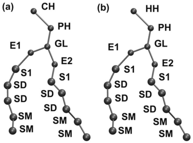
MS-CG models for (a) DOPC; and (b) DOPE.

The water solvent is entirely removed, i.e., effectively integrated out in the MS-CG model to achieve better computational efficiency. Thus, the solvent effects are implicitly reflected in the CG forces acting on the lipids only, so the final MS-CG force field for lipids is a “solvent free” force field. An more detailed analysis of building such solvent-free MS-CG force fields can be found in a forthcoming paper.³⁹

3. Results and Discussion

A. Reference All-atom MD Simulation

The present all-atom 1:1 DOPC/DOPE mixed bilayer contains 128 lipids and 4142 water molecules. Each leaflet of the bilayer is made of 32 DOPC and 32 DOPE and in the starting configuration these lipids were distributed randomly in the corresponding leaflet. The lipid force field parameters were taken from Berger et al.⁴⁰ Water molecules were simulated using the SPC model,⁴¹ and a 2 fs time step was implemented to all MD simulations. The Lennard-Jones (LJ) cutoff was set to 1.0 nm and the electrostatic interactions were simulated based on the particle-mesh Ewald (PME) method.⁴² For constraints, a linear constraint solver (LINCS) algorithm⁴³ was applied except that the SETTLE algorithm⁴⁴ was used for rigid water molecules. After energy minimization the system was run under the constant NPT ensemble for 20 ns, with pressure 1.01 bar and temperature 310 K. The Nose-Hoover thermostat⁴⁵ and the Parrinello-Rahman^46,47 pressure coupling method were applied. The average area per headgroup calculated from the last 10 ns of the constant NPT simulation was 0.567 nm², consistent with the result from de Vries et al.¹⁹ A 30 ns constant NVT run was then conducted after the constant NPT simulation with the same temperature, and the last 20 ns of the NVT trajectory was used for calculating reference forces in the MS-CG procedure. All atomistic and CG simulations in this article were performed using the GROMACS MD package.⁴⁸

B. MS-CG Procedure and Results

Reference forces in eq. (1) were calculated based on 20000 MD frames from the all-atom simulation. MS-CG forces were interpolated by B-spline basis functions as described earlier. For non-bonded interactions, B-splines functions with the order k=6 and the grid point number Nbreak=21 were implemented. The bonded forces in the matrix equation were not used in the final force field, replaced instead by the inverse Boltzmann fitting results as outlined previously. Thus a less accurate B-spline interpolation with k=4 and Nbreak=11 was used for the bonded forces in order to enhance computational efficiency. The MS-CG least squares problem was then solved using the normal matrix equation. First, the normal equation was built based on the information from the whole atomistic MD trajectory, and then the singular value decomposition (SVD) method was applied to solve the normal equation. The final B-spline force results were interpolated and integrated to obtain force field potential tables. Performance on an Intel Xeon workstation for the MS-CG calculation with the new B-spline basis functions shows that the computational speed roughly increased an order of magnitude and the memory cost reduced by a factor of five, compared with those from calculations using the original MS-CG algorithm with cubic spline basis sets.

For force field bonded interactions, the harmonic approximation was applied:

$$V\left(r\right)=\frac{1}{2}{k}_r{(r-r_0)}^2,$$ (4)

$$V\left(\theta \right)=\frac{1}{2}{k}_{\theta }{(\theta -{\theta }_0)}^2$$ (5)

where V(r) and V(θ) are bond/angle potentials; k_r and k_θ are bond/angle force constants; and r₀ and θ₀ are equilibrium distances/angles. These bonded force field parameters were determined by inverse Boltzmann fitting of the atomistic bond/angle distributions. The environmental effect correction was also applied for the bonded parameter results.³⁸ In order to perform the inverse Boltzmann fitting at the CG level, the all-atom trajectory was first converted to a “CG trajectory” by replacing atom coordinates by corresponding center of mass coordinates calculated based on the CG site definition. This “CG trajectory” was also used to calculate various all-atom bilayer properties including the RDFs in the later all-atom/CG comparisons of structural properties. Force field parameters for the bonded interactions are listed in Table 1.

Table 1.

Force constants and equilibrium distances/angles in the MS-CG force field. The errors for these force field parameters are less than 5% as estimated by the block average method.

Bond type	kr[kJ/(mol•nm)]	r0 (nm)
CH-PH	7.91×103	0.435
HH-PH	1.97×104	0.329
PH-GL	1.33×104	0.347
GL-E1	2.72×104	0.332
GL-E2	8.68×103	0.368
E1-S1	3.68×103	0.406
E2-S1	4.03×103	0.409
S1-SD	7.68×103	0.341
SD-SD	1.17×104	0.331
SD-SM	7.77×103	0.338
SM-SM	8.03×103	0.345

Angle type	kθ[kJ/(mol•rad)]	θ0 (deg)
CH-PH-GL	34.0	127.9
HH-PH-GL	74.6	115.8
PH-GL-E1	43.8	130.0
PH-GL-E2	31.1	125.0
E1-GL-E2	32.1	122.8
GL-E1-S1	23.0	142.9
GL-E2-S1	22.1	142.1
E1-S1-SD	18.8	159.4
E2-S1-SD	20.8	157.1
S1-SD-SD	40.2	146.6
SD-SD-SM	36.2	145.0
SD-SM-SM	23.5	158.2

Selected MS-CG force results are shown in Figure 2, while additional force results are similar to those from Izvekov and Voth.^30,32 Compared to previous DMPC results using cubic spline interpolation, the forces in this work are smoother, indicating noise has been filtered by the B-spline treatment. However, for certain pair interactions with relatively worse sampling, there are still obvious fluctuations in the force curves, implying some numerical uncertainty. The condition number from the SVD results was in the order of 10⁵, which is within the range for good numerical stability in double precision computations.³⁵

Figure 2.

Effective pairwise non-bonded forces (top) and potentials (bottom) between selected CG interaction sites. The approximate error bars in these force curves are about 5-10% of the force value calculated from block averages. See Figure 1 for CG site definitions.

The CG force field interactions displayed in Figure 2(a) show same-lipid preferences. The CHHH interaction is the most repulsive among the three types of pair interactions between the CH/HH sites. This trend is more obvious by observing the potential curves in the same figure. In the original all-atom force field, the value of the CH-HH interaction should be between those of CH-CH and HH-HH interactions due to the LJ combination rules. Thus the MS-CG results of CH/HH headgroup interactions contain various free energy effects from all-atom simulations. It should be noted that due to the relatively small force differences among the three interactions, the final lipid distribution may also be influenced by other effects such as the headgroup-tail area mismatch⁴⁹ as well as different PC/PE headgroup conformations reflecting headgroup hydration.¹⁹

The interaction between lipid headgroups/linker and different tail CG sites S1/SD are also shown in Figures 2(b) and (c). While the S1 type CG site contains three saturated carbons, there is one unsaturated carbon atom in each SD site. Compared to the CH-S1 interaction, the CH-SD interaction is by far more attractive. A similar trend has been found for the interaction between site GL and the two tail sites. Because the LJ parameters for tail carbons in the all-atom MD are identical, these effective differences come basically from free energy effects related to chain configurations. These interactions may affect the tail ordering in CG simulations and roughly reflect the double-bond effect in all-atom MD simulations. Resulting order parameter data will be discussed later. The results shown in Figure 2 illustrate the power of the MS-CG method in revealing the form of the effective condensed phase interactions between the CG sites and hence can also serve as an “analysis tool” for such interactions.

C. CG bilayer simulation and structural properties

Two bilayer systems were simulated using the MS-CG force field. The first one was a small bilayer that was identical to the one in the all-atom simulation except that water molecules were effectively removed in the MS-CG model. This system was simulated in a constant NVT ensemble for 1000 ns under the same conditions as those in the atomistic simulation. All CG structural properties for comparison to atomistic ones were calculated from the output MD trajectory of this system. The configuration of the second system contained 512 lipids and was created by replicating the small bilayer in two dimensions to four times the size of the original one. The larger system was simulated for 300 ns in order to observe equilibrated 2D distribution of the lipid molecules. Since the MS-CG model is solvent free, it is possible to simulate the two systems at a relatively long time scale with moderate computer resources. Snapshots of the equilibrated systems are shown in Figure 3. Both two bilayers were stable for the length of the simulations

Figure 3.

Snapshots of equilibrated bilayer configurations for (a) the 128 lipid system and (b) the 512 lipid system. Color scheme: purple for CH; blue for HH; orange for PH; red for E1/E2; green for S1/SD/SM. See Figure 1 for CG site definitions.

In a CG simulation the lipid lateral diffusion is generally much faster than that in atomistic simulations. Thus the mixing equilibrium is easier to achieve and the resulting lateral distribution of lipids is different compared to the distribution resulting from highly trapped lipid lateral dynamics in atomistic MD simulations. The RDF results involving CH and HH sites are therefore expected to reflect the above effect of PC/PE mixing and the corresponding data are shown in Figure 4. It is shown in Figure 4 that, as expected, the three CG RDFs are slightly different compared to atomistic counterparts. In Figure 4 more same-lipid preference can be observed in the CG RDF results. When compared to there atomistic MD counterparts, there is an extra peak at closer distance in the CG CH-CH RDF. For the CG HH-HH RDF, higher peaks are also observed. Additionally the CG RDF peak for the cross interaction CH-HH is lower than that from the all-atom MD model. This RDF data suggests that compared to the atomistic distributions, the lipids tend to stay close to the same type lipids in the CG simulations. The lateral lipid distribution will be discussed in detail later in this article.

Figure 4.

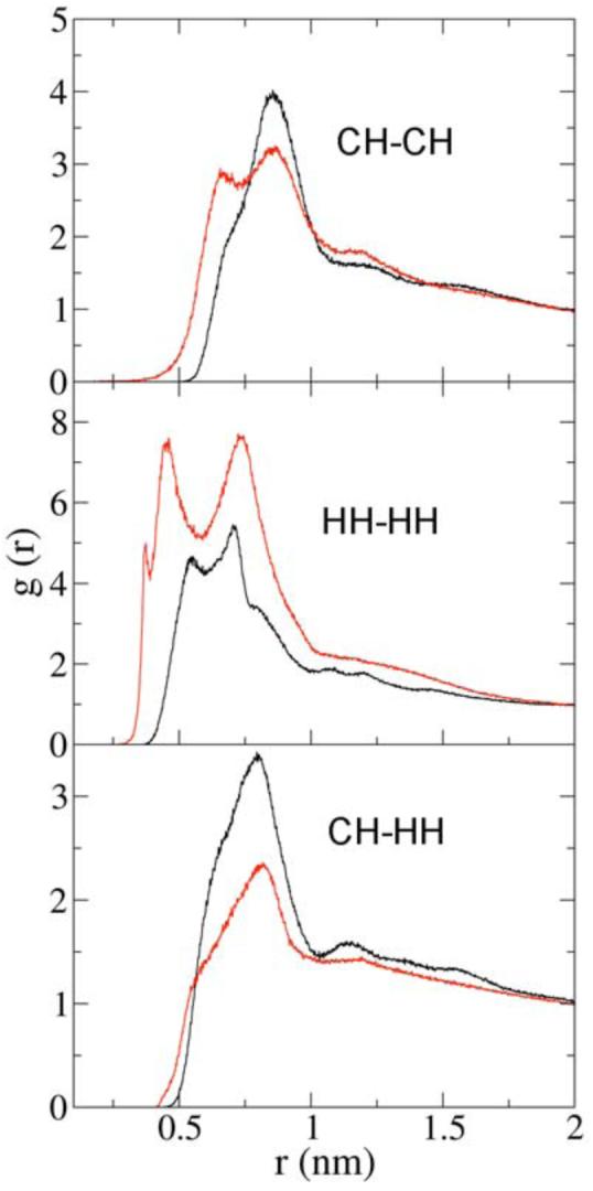
CH-CH, HH-HH, and CH-HH RDFs from the CG simulation (red) and the all-atom simulation (black). See Figure 1 for CG site definitions.

In all-atom MD simulations of mixed bilayers, various structural properties (which are not particularly associated to lipid mixing), such as area per headgroup and single lipid configuration, are usually considered to be equilibrated. Therefore, the remaining CG RDF results are expected to be consistent with atomistic MD results because the MS-CG method has been shown to be able to reproduce all-atom RDFs, both theoretically⁵⁰ and in practice.^30-32 Selected radial distribution functions of both all-atom and CG simulations are show in Figure 5. From Figure 5 the CG RDF results for most pairs are in good agreement with their all-atom MD counterparts. This indicates that the MS-CG solvent free bilayer model is able to capture the free energy landscape underlying the atomistic simulations. However, aside from select RDFs related to PC/PE interactions, which have been discussed, some disagreements in the CG/atomistic results remain in Figure 5. These discrepancies can be explained by several reasons: first, some many-body effects have been missed because of the pairwise interaction approximation used in the MS-CG approach. These many-body effects are especially important for water and other groups which can form hydrogen bonds, and they cause less perfect structural properties in the solvent free bilayer model. Second, the harmonic approximation was applied to bonded interactions, which may not always be accurate. Finally, the least-squares problem in the MS-CG method is usually an ill-posed problem. Although it can be solved by various methods for high condition number problems such as the SVD implemented in this work, some numerical instabilities remain.

Figure 5.

Selected site-site RDFs from the CG simulation (solid lines) and the atomistic simulation (dashed lines). See Figure 1 for CG site definitions.

Part of the bond distribution data are shown in Figure 6. The atomistic bond and angle distributions are qualitatively reproduced by the CG force field. The simple harmonic potential form in the CG force field was chosen because it is supported by most current MD packages. There are, however, some bond/angle distributions with multiple maxima which cannot be precisely represented by harmonic bond/angle potential. In practice, even high order analytical potentials such as the quartic potential can not capture most of these distributions. In future work, tabulated bond/angle potential will be applied in order to obtain more accurate bonded CG potentials.

Figure 6.

Selected bond and angle distributions from the CG simulation (solid line) and the atomistic simulation (dashed line). See Figure 1 for CG site definitions.

Selected lipid bilayer density profiles along the z-axis are shown in Figure 7. These density profiles in the CG simulation are in good agreement with atomistic MD results. It can also be inferred from headgroup density results that the atomistic bilayer thickness is maintained in the CG bilayer, though there is no explicit water present in the MS-CG model. Compared with the HH density profile, the CH sites have larger z-values, reflecting a stronger hydration in the atomistic MD simulation. This density profile difference between PC/PE headgroups is consistent with the simulation results by de Vries et al¹⁹., and the hydrogen bonding difference related to it may play a role in the determination of CG interactions associated to headgroups.

Figure 7.

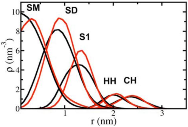
Z-density profiles for selected sites from the CG simulation (black) and the atomistic simulation (red). Zero means the bilayer center for the abscissa. See Figure 1 for CG site definitions.

The lipid tail order information can be obtained by calculating the second-order parameter $P_2=\frac{1}{2}(3>{\cos }^2(\theta )>-1)$ where θ is an angle between the bond studied and the bilayer normal. If P₂ = 1, the bond is parallel to the bilayer normal; P₂ = -0.5 indicates that the bond is perpendicular to the normal; P₂ = 0 means that the bond orientation is completely disordered. The comparison between CG and all-atom P₂ results is shown in Figure 8. The magnitudes of CG/all-atom differences in P₂ values are similar to those from Izvekov and Voth.³² For the bonds in lipid tails, the P₂ values are much more close to 0 compared to the DMPC results from the latter paper. This shows the effect of unsaturated bonds which increases the tail disorder. Although there are no explicit trans/cis conformations due to the limited resolution in the CG lipid model, the tail order is qualitatively retained in CG simulations as shown by the P₂ data. This feature of the present MS-CG lipid model is important since it is believed that the lipid tail order related to tail saturation plays a key role in membrane phase behavior for various mixed lipid systems containing both saturated and unsaturated lipids.^51,52

Figure 8.

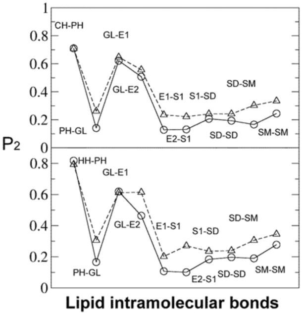
P₂ order parameters of bonds with respect to bilayer normal from the CG simulation (solid line, circle) and the atomistic simulation (dashed line, triangle). Upper plot: DOPC lipids; lower plot: DOPE lipids. The lines are meant to guide the eye. See Figure 1 for CG site definitions.

The lateral diffusion coefficient can be calculated from the mean square displacement (MSD) plot. The MSD plot of the PH site which represents the lateral mobility of lipid phosphate group is shown in Figure 9. Unlike the atomistic MD results of de Vries et al¹⁹ in which MSD curves exhibit nonlinear behavior indicating that the lipids were trapped in local minima, the MSD in the MS-CG simulation is mostly in the linear region from which the lateral diffusion coefficient can be easily calculated. The effective lateral diffusion coefficient of PH site is 4×10^-10 m²/s calculated based on the slope of the linear region of the MSD curve. Although a corresponding atomistic MD value is not available because linearity can not be reached in its MSD plot, the effective CG lateral diffusion coefficient is estimated to be roughly more than one order of magnitude larger than the corresponding lateral diffusion coefficient in all-atom simulations. Here the word “effective” is used since in CG simulations the dynamics are usually much faster and various corresponding dynamical quantities can not be compared with all-atom MD or experimental values before appropriate scaling⁵³ or the addition of frictional forces.⁵⁴ The CG lateral diffusion coefficient result in this work is similar to the result from Nielsen et al for a DMPC system in which the CG lateral diffusion coefficient was roughly 100 times the atomistic one.⁵³ This fast dynamics may be due to the much smoother free energy landscape in CG simulations. Although the CG dynamical properties are not consistent with all-atom results, various structural and thermodynamic quantities from MS-CG force field are in principle in agreement with their atomistic counterparts.^33,50 Therefore, it is desired to have this faster dynamics in the CG simulation in order to observe the equilibrated structural results on a shorter simulation time scale.

Figure 9.

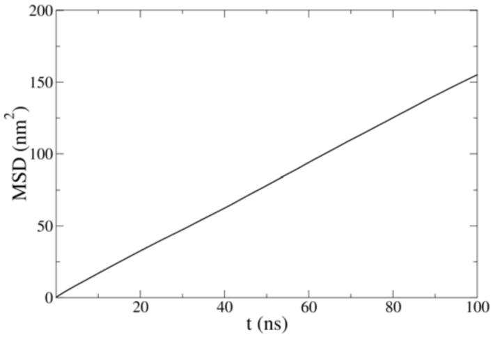
Lateral mean square displacement of the PH sites from the MS-CG simulation.

D. Lipid lateral distribution and clustering

The larger bilayer system with 512 lipids was chosen for the study of lipid lateral distributions in order to reduce possible boundary artifacts that could occur in the original smaller bilayer system. Since our CG force field is derived from an all-atom system of 128 lipids, in principle, it is not guaranteed to reflect all bilayer properties related to larger time and length scales due to the limited system size and simulation time for the atomistic system. For example, the membrane undulations with large wavelength in the CG bilayer simulations might require additional validation. However, as shown earlier the MS-CG force field reflects the many body potential of mean force between CG sites so key features of related inter and intra molecular lipid-lipid interactions in the all-atom system therefore can be retained in the MS-CG force field. Since these lipid-lipid interactions and related free energy effects are believed to be important to system phase properties, a larger bilayer system was chosen in CG simulations in order to observe the phase behavior as a result of short ranged CG interactions.

A top view of the trajectory after equilibration is shown in Figure 10. It is seen from the snapshot that there are several visible lipid clusters present on the bilayer surface. By analyzing the whole MD trajectory, it was found that small clusters made of the same lipid appeared during the whole equilibrated trajectory and there were frequent lipid exchanges between clusters and isolated lipids due to the fast lipid lateral dynamics in the CG simulation. In order to test the degree of equilibration of the lipid lateral distribution, test MS-CG simulations were performed starting from an initial configuration in which DOPC and DOPE occupied one half of the simulation box respectively. The system evolved into a similar small cluster configuration within 50 ns, indicating that equilibrium can be reached very rapidly in the CG simulations. The unevenly distributed lipids can be related to the CG force field parameters for headgroup-headgroup interactions. But as discussed previously, other effects such as the headgroup-tail area mismatch can play an important role in determining the lipid distribution.

Figure 10.

Topview of one leaflet of the mixed bilayer showing the equilibrated lateral PC/PE distribution. Only the PH sites are shown for clarity. The red dots represent DOPC and the blue dots represent DOPE.

In order to analyze the lipid cluster distribution, the probability distribution as a function of cluster size is shown in Figure 11 for the DOPC clusters. The DOPE cluster distribution has a similar shape and is not shown here. In the calculation of the DOPC cluster distribution, the x/y coordinates of the DOPC PH sites are used to represent the lateral position of each lipid. By observing the two dimensional PH-PH RDF on the xy-plane (not shown), the first minimum on the PH-PH RDF is seen to be at 1.0 nm, thus this distance can be used as the cutoff to determine if two lipids are clustered. After building the connectivity information between any two lipids, the cluster size distribution can be calculated based on the method from Sevick et al.⁵⁵ From the result shown in Figure 11, there is a considerable probability for small PC clusters of the size between 2 to 20 though the isolated lipid has the highest probability. This probability distribution is consistent with a direct observation of the snapshot in Figure 10. The probability for a cluster size above 50 is near zero, indicating that no obvious domains at a length scale above nanometers are found in the MS-CG simulation.

Figure 11.

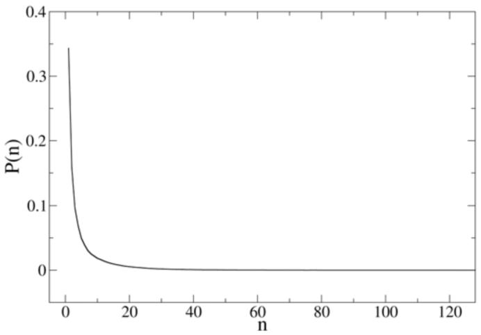
Probability distribution of DOPC cluster size.

From the cluster distribution results, a super-lattice proposal¹⁷ is not supported, nor is the concept of domain formation. It should be noted that the DOPC/DOPE system in this work follows the study from de Vries et al.,¹⁹ but it is different from the POPC/POPE system used in the two experimental studies which support the two ideas described above.^17,18 Experimental results for the DOPC/DOPE system are currently unavailable. Because each DOPC/DOPE molecule has two unsaturated tails which occupy a larger area than that of POPC/POPE, the feature of the headgroup/tail area mismatch in the DOPC/DOPE system may be different compared to that in the POPC/POPE system. This may be the reason that no super-lattice structure was formed in the CG simulations. Interestingly, in the work by Ahn and Yun, they suggested the possibility of “partial” domain formation because their results for the excimer to monomer (E/M) fluorescence ratio varied slightly from the typical domain formation values.¹⁸ Although detailed structural information can not be observed directly in these fluorescence experiments, it is possible that the partial domain formation behavior suggested by these experiments may be connected to the small clusters found in the present CG simulations.

4. Conclusions

The modified MS-CG method using B-spline basis functions to represent the CG forces has been shown in this work to efficiently produce a solvent-free multi-component CG lipid bilayer model with good accuracy for a DOPC/DOPE system. Various structural properties from the MS-CG trajectories agree well with their atomistic MD counterparts. By applying the new basis set, the number of unknown coefficients in the MS-CG least squares problem can be greatly decreased. Thus the required computer time and memory are reduced dramatically, making it feasible to apply the MS-CG method to more complicated biomolecular systems in future studies.

The CG simulation trajectories were used to examine the lipid lateral distribution. Because of the high efficiency of the solvent-free MS-CG model, long time scale simulations can be performed. The lateral dynamics of lipids was observed to reach the linear MSD region due to the long simulation time and smoother free energy surface in the CG simulations. The simulation results for DOPC/DOPE support neither the super-lattice hypothesis nor domain formation on the nanometer scale. Instead, small clusters consisting of the same type of lipid are observed, which possibly supports prior experimental results indicating partial domain formation.

Since the MS-CG force field is able to capture the lipid tail ordering of unsaturated lipids from all-atom MD simulations as shown earlier, it will be promising to apply the MS-CG approach to typical domain forming systems that usually contain both saturated and unsaturated lipids. Membrane systems of different molecular components and ratios can be easily simulated by conventional all-atom force fields and the MS-CG models are able to be systematically constructed based on the corresponding all-atom MD results. Liu et al. also demonstrated that the MS-CG method showed good transferability over different thermodynamics conditions for a carbohydrate system.⁵⁶ Therefore, it may be possible to develop CG models transferable to different membrane compositions and other experimental conditions using the MS-CG approach. Applications of the MS-CG method to bilayer systems with stronger evidence for domain formation are currently underway.

References

- (1).Engelman DM. Nature. 2005;438:578. doi: 10.1038/nature04394. [DOI] [PubMed] [Google Scholar]
- (2).Maxfield FR, Tabas I. Nature. 2005;438:612. doi: 10.1038/nature04399. [DOI] [PubMed] [Google Scholar]
- (3).Dupuy AD, Engelman DM. Proc. Natl. Acad. Sci. U. S. A. 2008;105:2848. doi: 10.1073/pnas.0712379105. [DOI] [PMC free article] [PubMed] [Google Scholar]
- (4).Lingwood D, Ries J, Schwille P, Simons K. Proc. Natl. Acad. Sci. U. S. A. 2008;105:10005. doi: 10.1073/pnas.0804374105. [DOI] [PMC free article] [PubMed] [Google Scholar]
- (5).Brown DA, London E. J. Biol. Chem. 2000;275:17221. doi: 10.1074/jbc.R000005200. [DOI] [PubMed] [Google Scholar]
- (6).Binder WH, Barragan V, Menger FM. Angew. Chem.-Int. Edit. 2003;42:5802. doi: 10.1002/anie.200300586. [DOI] [PubMed] [Google Scholar]
- (7).Marsh D. Biochim. Biophys. Acta-Rev. Biomembr. 1996;1286:183. doi: 10.1016/s0304-4157(96)00009-3. [DOI] [PubMed] [Google Scholar]
- (8).Haque ME, McIntosh TJ, Lentz BR. Biochemistry. 2001;40:4340. doi: 10.1021/bi002030k. [DOI] [PubMed] [Google Scholar]
- (9).Yang L, Ding L, Huang HW. Biochemistry. 2003;42:6631. doi: 10.1021/bi0344836. [DOI] [PubMed] [Google Scholar]
- (10).Kasson PM, Pande VS. PLoS Comput. Biol. 2007;3:2228. doi: 10.1371/journal.pcbi.0030220. [DOI] [PMC free article] [PubMed] [Google Scholar]
- (11).Scarlata S, Gruner SM. Biophys. Chem. 1997;67:269. doi: 10.1016/s0301-4622(97)00053-7. [DOI] [PubMed] [Google Scholar]
- (12).Hunter GW, Negash S, Squier TC. Biochemistry. 1999;38:1356. doi: 10.1021/bi9822224. [DOI] [PubMed] [Google Scholar]
- (13).Lewis JR, Cafiso DS. Biochemistry. 1999;38:5932. doi: 10.1021/bi9828167. [DOI] [PubMed] [Google Scholar]
- (14).Botelho AV, Gibson NJ, Thurmond RL, Wang Y, Brown MF. Biochemistry. 2002;41:6354. doi: 10.1021/bi011995g. [DOI] [PubMed] [Google Scholar]
- (15).Alves ID, Salgado GFJ, Salamon Z, Brown MF, Tollin G, Hruby VJ. Biophys. J. 2005;88:198. doi: 10.1529/biophysj.104.046722. [DOI] [PMC free article] [PubMed] [Google Scholar]
- (16).McIntosh TJ. Chem. Phys. Lipids. 1996;81:117. doi: 10.1016/0009-3084(96)02577-7. [DOI] [PubMed] [Google Scholar]
- (17).Cheng KH, Ruonala M, Virtanen J, Somerharju P. Biophys. J. 1997;73:1967. doi: 10.1016/S0006-3495(97)78227-4. [DOI] [PMC free article] [PubMed] [Google Scholar]
- (18).Ahn T, Yun CH. Arch. Biochem. Biophys. 1999;369:288. doi: 10.1006/abbi.1999.1376. [DOI] [PubMed] [Google Scholar]
- (19).de Vries AH, Mark AE, Marrink SJ. J. Phys. Chem. B. 2004;108:2454. [Google Scholar]
- (20).Joannis J, Jiang Y, Yin FC, Kindt JT. J. Phys. Chem. B. 2006;110:25875. doi: 10.1021/jp065734y. [DOI] [PubMed] [Google Scholar]
- (21).Illya G, Lipowsky R, Shillcock JC. J. Chem. Phys. 2006;125 doi: 10.1063/1.2353114. [DOI] [PubMed] [Google Scholar]
- (22).Laradji M, Kumar PBS. J. Chem. Phys. 2005;123 doi: 10.1063/1.2102894. [DOI] [PubMed] [Google Scholar]
- (23).Marrink SJ, Risselada HJ, Yefimov S, Tieleman DP, de Vries AH. J. Phys. Chem. B. 2007;111:7812. doi: 10.1021/jp071097f. [DOI] [PubMed] [Google Scholar]
- (24).Bennun SV, Longo M, Faller R. J. Phys. Chem. B. 2007;111:9504. doi: 10.1021/jp072101q. [DOI] [PubMed] [Google Scholar]
- (25).Faller R, Marrink SJ. Langmuir. 2004;20:7686. doi: 10.1021/la0492759. [DOI] [PubMed] [Google Scholar]
- (26).Risselada HJ, Marrink SJ. Proc. Natl. Acad. Sci. U. S. A. 2008;105:17367. doi: 10.1073/pnas.0807527105. [DOI] [PMC free article] [PubMed] [Google Scholar]
- (27).Shelley JC, Shelley MY, Reeder RC, Bandyopadhyay S, Klein ML. J. Phys. Chem. B. 2001;105:4464. [Google Scholar]
- (28).Meyer H, Biermann O, Faller R, Reith D, Muller-Plathe F. J. Chem. Phys. 2000;113:6264. [Google Scholar]
- (29).Murtola T, Falck E, Patra M, Karttunen M, Vattulainen I. J. Chem. Phys. 2004;121:9156. doi: 10.1063/1.1803537. [DOI] [PubMed] [Google Scholar]
- (30).Izvekov S, Voth GA. J. Phys. Chem. B. 2005;109:2469. doi: 10.1021/jp044629q. [DOI] [PubMed] [Google Scholar]
- (31).Izvekov S, Voth GA. J. Chem. Phys. 2005;123 doi: 10.1063/1.1961443. [DOI] [PubMed] [Google Scholar]
- (32).Izvekov S, Voth GA. J. Chem. Theory Comput. 2006;2:637. doi: 10.1021/ct050300c. [DOI] [PubMed] [Google Scholar]
- (33).Noid WG, Chu J-W, Ayton GS, Krishna V, Izvekov S, Voth GA, Das A, Andersen HC. J. Chem. Phys. 2008;128:244114. doi: 10.1063/1.2938860. [DOI] [PMC free article] [PubMed] [Google Scholar]
- (34).Noid WG, Liu P, Wang Y, Chu J-W, Ayton GS, Izvekov S, Andersen HC, Voth GA. J. Chem. Phys. 2008;128:244115. doi: 10.1063/1.2938857. [DOI] [PMC free article] [PubMed] [Google Scholar]
- (35).Press WH, Teukolsky SA, Vettering WT, Flannery BP. Numerical Recipes in C, The Art of Scientific Computing, Second Edition. Cambridge University Press; 1997. [Google Scholar]
- (36).Lawson CL, Hanson RJ. Solving Least Squares Problems. Prentice-Hall; Englewood Cliffs, NJ: 1974. [Google Scholar]
- (37).de Boor C. A Practical Guide to Splines, Revised Edition. Springer; 2001. [Google Scholar]
- (38).Wang YT, Izvekov S, Yan TY, Voth GA. J. Phys. Chem. B. 2006;110:3564. doi: 10.1021/jp0548220. [DOI] [PubMed] [Google Scholar]
- (39).Izvekov S, Voth GA.In preparation
- (40).Berger O, Edholm O, Jahnig F. Biophys. J. 1997;72:2002. doi: 10.1016/S0006-3495(97)78845-3. [DOI] [PMC free article] [PubMed] [Google Scholar]
- (41).Berendsen HJC, Postma JPM, Van Gunsteren WF, Hermans J. In: Intermolecular Forces. Pullman B, editor. D. Reidel Publishing Company; Dordrecht: 1981. [Google Scholar]
- (42).Essmann U, Perera L, Berkowitz ML, Darden T, Lee H, Pedersen LG. J. Chem. Phys. 1995;103:8577. [Google Scholar]
- (43).Hess B, Bekker H, Berendsen HJC, Fraaije J. J. Comput. Chem. 1997;18:1463. [Google Scholar]
- (44).Miyamoto S, Kollman PA. J. Comp. Chem. 1992;13:952. [Google Scholar]
- (45).Nose S. J. Chem. Phys. 1984;81:511. [Google Scholar]
- (46).Nose S, Klein ML. Mol. Phys. 1983;50:1055. [Google Scholar]
- (47).Parrinello M, Rahman A. J. Appl. Phys. 1981;52:7182. [Google Scholar]
- (48).Lindahl E, Hess B, van der Spoel D. J. Mol. Model. 2001;7:306. [Google Scholar]
- (49).Somerharju P, Virtanen JA, Cheng KH. BBA-Mol. Cell. Biol. Lipids. 1999;1440:32. doi: 10.1016/s1388-1981(99)00106-7. [DOI] [PubMed] [Google Scholar]
- (50).Noid WG, Chu JW, Ayton GS, Voth GA. J. Phys. Chem. B. 2007;111:4116. doi: 10.1021/jp068549t. [DOI] [PMC free article] [PubMed] [Google Scholar]
- (51).Silvius JR. Biochim. Biophys. Acta-Biomembr. 2003;1610:174. doi: 10.1016/s0005-2736(03)00016-6. [DOI] [PubMed] [Google Scholar]
- (52).Elliott R, Katsov K, Schick M, Szleifer I. J. Chem. Phys. 2005;122 doi: 10.1063/1.1836753. [DOI] [PubMed] [Google Scholar]
- (53).Nielsen SO, Lopez CF, Srinivas G, Klein ML. J. Phys.-Condes. Matter. 2004;16:R481. [Google Scholar]
- (54).Izvekov S, Voth GA. J. Chem. Phys. 2006;125 doi: 10.1063/1.2360580. [DOI] [PubMed] [Google Scholar]
- (55).Sevick EM, Monson PA, Ottino JM. J. Chem. Phys. 1988;88:1198. doi: 10.1103/physreva.38.5376. [DOI] [PubMed] [Google Scholar]
- (56).Liu P, Izvekov S, Voth GA. J. Phys. Chem. B. 2007;111:11566. doi: 10.1021/jp0721494. [DOI] [PubMed] [Google Scholar]