

Abstract
The ferret has become a model animal for studies exploring the development of the visual system. However, little is known about the receptive-field structure and response properties of neurons in the adult visual cortex of the ferret. We performed single-unit recordings from neurons in layer 4 of adult ferret primary visual cortex to determine the receptive-field structure and visual-response properties of individual neurons. In particular, we asked what is the spatiotemporal structure of receptive fields of layer 4 neurons and what is the orientation selectivity of layer 4 neurons? Receptive fields of layer 4 neurons were mapped using a white-noise stimulus; orientation selectivity was determined using drifting, sine-wave gratings. Our results show that most neurons (84%) within layer 4 are simple cells with elongated, spatially segregated, ON and OFF subregions. These neurons are also selective for stimulus orientation; peaks in orientation-tuning curves have, on average, a half-width at half-maximum response of 21.5 ± 1.2° (mean ± SD). The remaining neurons in layer 4 (16%) lack orientation selectivity and have center/surround receptive fields. Although the organization of geniculate inputs to layer 4 differs substantially between ferret and cat, our results demonstrate that, like in the cat, most neurons in ferret layer 4 are orientation-selective simple cells.
INTRODUCTION
Neurons in layer 4 of primary visual cortex are the main target of axons arising from the lateral geniculate nucleus (LGN) of the thalamus (Bullier and Henry 1979; Hendrickson et al. 1978; Hubel and Wiesel 1972). Based on this input, layer 4 neurons represent the first stage of visual processing in the cerebral cortex. In the cat, where the physiology of layer 4 neurons has been studied most extensively, there is a dramatic transformation from the receptive-field structure of geniculate inputs to that of layer 4 neurons. While geniculate neurons have center/surround receptive fields with circular centers (ON or OFF) and antagonistic surrounds (Hubel and Wiesel 1961), their target neurons—simple cells—in cortical layer 4 have elongated receptive fields with adjacent ON and OFF subregions (Bullier and Henry 1979; Gilbert 1977; Hubel and Wiesel 1962; Kelly and Van Essen 1974). As might be expected from the spatial organization of the simple cell receptive field, simple cells respond best to appropriately oriented bars or edges of light (Gilbert 1977; Henry et al. 1974; Hubel and Wiesel 1962). While the receptive-field structure that defines the simple cell is characteristic for the majority of neurons in layer 4 of cat visual cortex (Gilbert 1977; Hubel and Wiesel 1962; see also Henry et al. 1979), the simple cell receptive field is not universal to layer 4 in all mammals. For instance, center/surround receptive fields dominate in layer 4 of tree shrew visual cortex and establish one end of a spectrum of receptive fields encountered in layer 4C of macaque visual cortex (Blasdel and Fitzpatrick 1984; Hawken and Parker 1984; Hubel and Wiesel 1977; Kretz et al. 1986; Leventhal et al. 1995; Ringach et al. 2002). Even among carnivores, it remains to be determined whether the simple cell receptive field should be viewed as the rule or the exception for neurons in layer 4.
Due to its close relation to the cat, yet dramatically earlier birth, the ferret has increasingly becoming a model system for studying the early development of the visual system. Despite the widespread use of young ferrets for addressing questions about neural development, our understanding of the visual physiology in the adult ferret is quite limited. In particular, we lack any knowledge of the spatial organization of layer 4 receptive fields. For instance, do layer 4 neurons have center/ surround, simple or complex receptive fields? Based on reports that ON and OFF geniculate axons terminate in nonoverlapping patches within layer 4 of the ferret (Zahs and Stryker 1988) and layer 4 neurons with similar ON versus OFF preferences tend to cluster in the mink (LeVay et al. 1987), one might expect to find patches of layer 4 cells in the ferret with center/surround receptive fields of the same sign or patches with elongated single-subunit receptive fields (Kato et al. 1978). Contrary to this prediction, however, optical imaging studies have failed to identify functional ON or OFF patches in supragranular cortex (Chapman and Godecke 2002). Thus it remains to be determined whether or not individual layer 4 neurons in the ferret have access to information from both the ON and OFF pathways.
A separate but related issue is whether or not layer 4 neurons in the ferret display orientation selectivity. To our knowledge, only two studies have examined orientation selectivity specifically among layer 4 neurons (Chapman and Stryker 1993; Weliky and Katz 1997), and both of these studies report a broad range of responses. Because the ferret has become a model system for studying the development of orientation selectivity in particular (reviewed in Chapman et al. 1999), it is critical to determine where in the cortical circuit orientation selectivity first emerges. Many models for the development of orientation selectivity are based on correlated activity among geniculate inputs to neurons in cortical layer 4 (Erwin and Miller 1998; Katz and Shatz 1996; Miller 1994; Miller et al. 1999; Mooney et al. 1996; Tavazoie and Reid 2000). If neurons in layer 4 of ferret visual cortex indeed display orientation selectivity, then this finding would be consistent with these correlation-based models.
We examined the receptive-field structure and response properties of individual neurons in layer 4 of primary visual cortex in the adult ferret. Our results show that most neurons in layer 4 of ferret visual cortex are orientation-selective simple cells similar to those in the cat. Unlike in the cat, however, a small population of neurons in ferret layer 4 lacked orientation selectivity and had center/surround receptive fields. For the population of simple cells, measured values for size and shape of simple-cell subregions as well as degree of orientation selectivity were statistically indistinguishable from values previously reported for simple cells in layer 4 of cat visual cortex.
METHODS
Animal preparation
All surgical and experimental procedures conformed to National Institutes of Health and U. S. Department of Agriculture guidelines and were carried out with the approval of the Animal Care and Use Committee at the University of California, Davis. Eight adult ferrets (Mustela putorius furo) were used in this study. Surgical anesthesia was induced with an intramuscular injection of ketamine (40 mg/kg) and acepromazine (0.04 mg/kg). A tracheotomy was performed, and animals were placed in a stereotaxic apparatus where anesthesia was maintained with 1-1.5% isoflurane in oxygen and nitrous oxide (2:1). Body temperature was maintained at 37°C using a thermostatically controlled heating blanket. Temperature, electrocardiography (EKG), electroencephalography (EEG), and expired CO2 were monitored continuously throughout the experiment. Eyes were dilated with 1% atropine sulfate, fitted with appropriate contact lenses, and focused on a tangent screen located 76 cm in front of the animal. A midline scalp incision was made, and a small craniotomy was made above the primary visual cortex. All wound margins were infused with lidocaine.
Once all surgical procedures were complete, animals were paralyzed with vecuronium bromide (0.2 mg · kg-1 · h-1 iv) and ventilated mechanically. Proper depth of anesthesia was ensured throughout the experiment by monitoring the EEG for changes in slow-wave/ spindle activity and monitoring the EKG and expired CO2 for changes associated with a decrease in the depth of anesthesia.
Electrode-track reconstruction
At the end of each experiment, animals were given a lethal overdose of pentobarbital sodium (200 mg/kg). Once the EEG, heart rate, and CO2 levels indicated that the animal had expired, animals were perfused through the heart with saline followed by 4% paraformaldehyde in 0.1 M phosphate buffer (PB). After fixation, brains were rinsed in a 10% solution of sucrose in PB and immersed overnight in a 20% solution of sucrose in phosphate buffer. Brains were sectioned coronally at 60 βm on a freezing microtome. Sections were mounted onto gel-subbed slides, counterstained with thionin, dehydrated with alcohol, cleared with xylene, and coverslipped in permount. Electrode tracks, lesions (made during the experiment by passing 3 μA current for 10 s), and recording sites were reconstructed using a Nikon microscope. Reconstruction of electrode tracks was usually based on two or more lesions along the track. A Burleigh Instruments digital microdrive (Fishers, NY) was used to document the distance between lesions and recording sites as well as the depth of recording sites from the surface of the brain. In cases when all of the recorded cells were within 200 μm of each other, a single lesion was made at the midpoint of the recorded cells, after recording was completed.
Electrophysiological recordings and visual stimuli
Recordings were made from neurons in the primary visual cortex with tungsten in glass electrodes (Alan Ainsworth, London, UK). Spike times and waveforms were recorded to disk (with 100-μs resolution) by a PC running the Discovery software package (Data-wave Technologies, Longmont, CO). Spike isolation was confirmed with off-line waveform analysis and by the presence of a refractory period, as seen in the autocorrelograms (Alonso et al. 2001; Usrey and Reid 1999, 2000).
Receptive fields of cortical neurons were mapped quantitatively by reverse correlation (Jones and Palmer 1987; see Citron et al. 1981) using pseudorandom spatiotemporal white-noise stimuli (m-sequences) (Reid et al. 1997; Sutter 1987, 1992). The stimuli were created with an AT-Vista graphics card (Truevision, Indianapolis, IN) running at a frame rate of 128 Hz. The stimulus program was developed with subroutines from a runtime library, YARL, written by Karl Gegenfurtner. The mean luminance of the stimulus monitor (BARCO) was 40-50 cd/m2.
The white-noise stimulus (100% contrast) consisted of a 16 × 16 grid of squares (pixels) that were white or black one half of the time as determined by an m-sequence of length 215-1. The stimulus was updated either every frame of the display (7.8 ms), every other frame (15.6 ms) or every fourth frame (31.2 ms). The entire sequence (~4, 8, or 16 min) was often repeated several times. The size of individual pixels varied (from 0.75 to 1.5° on a side) depending on the receptive fields under study, which were between 5 and 15° eccentric. In most cases 8-24 pixels filled the receptive field.
Sinusoidal grating stimuli (100% contrast, peak spatial frequency) were also used to characterize the neurons under study. Neuronal responses to gratings (the first Fourier coefficient, or f1) drifting at 4 Hz were used to generate orientation-tuning curves. Gratings were presented at 16 different orientations (22° apart). For each orientation, gratings were shown for 4 s, followed by 1.6 s of mean gray. After the period of mean gray, a new grating was shown with a different orientation. Once all orientations were shown, the process was repeated four additional times.
Receptive-field mapping: reverse correlation
Spatiotemporal receptive-field maps (kernels) were calculated from the responses to the white-noise (m-sequence) stimulus by a reverse-correlation method (Reid et al. 1997; Sutter 1987, 1992; see Citron et al. 1981; Jones and Palmer 1987). For each delay between stimulus and response and for each of the 16 × 16 pixels, we calculated the average stimulus that preceded each spike (+1 for white, -1 for black). For each of the pixels, the kernel can also be thought of as the average firing rate of the neuron, above or below the mean, following the bright phase of the stimulus at that pixel (the impulse response). When normalized by the product of the bin width and the total duration of the stimulus, the result is expressed in units of spikes/s.
To assess the time course and magnitude of the response, it was necessary to identify the pixels in the strongest subregion of the receptive field. First, the largest single response was located: the position of greatest sensitivity at the most effective delay between stimulus and response. Next, the spatial extent of the subregion was defined as all contiguous spatial positions in this spatial receptive field that were the same sign as the strongest response and were >2.5 times the SD of the baseline noise. The baseline noise was taken as the SD of the kernel values for all pixels and for delays well beyond the peak response (140-187 or 280-374 ms). The impulse responses of all of the pixels in a given subregion were added together to yield the subregion's impulse response.
Parameters quantifying the impulse responses were calculated as follows. The time of maximum response, tmax, was calculated from the subregion impulse response. The rebound time, trebound, was defined as the first time, following tmax, that the response was opposite in sign from the maximum response. The peak magnitude—which quantifies the first phase of the response, the response before the rebound—was defined as the integral of the impulse response for all times before trebound. Finally, the rebound magnitude was defined as the integral of the impulse response for times greater than trebound (≤187 ms).
Fitting receptive-field maps
The reverse correlation maps were fitted with a 2 dimensional Gabor filter, g(x,y)
The orientation of the filter is captured by a polar coordinate transformation where X and Y are defined by the transformation
The origin of the filter within two-dimensional space is fitted with a spatial position offset
which allows us to fit the receptive field data for an arbitrary origin location. The Gabor filter carrier sine wave is composed of a spatial frequency parameter, sf, and a spatial phase offset parameter, φ.
All of the reverse correlation maps were fitted using an unconstrained minimization algorithm in Matlab (fminsearch, MathWorks, Natick, MA). The maps were initially fitted using a Gabor filter with a circular Gaussian envelope. Optimal values for carrier frequency, spatial offset position, and orientation (sf, φx, φy, and θ) were determined from the circular Gabor fits. Next these parameters were constrained to the values determined from the circular Gabor fits, and the maps were fitted again with an elliptical Gabor filter. The free parameters for the elliptical Gabor fits included the space constants (a and b) for the elliptical Gaussian envelope as well as and the carrier spatial phase (φ).
The receptive-field orientation, length, and width were estimated directly from the Gabor filter parameters θ, b, and a, respectively. Receptive-field subunits were also quantified from the Gabor-filterfitted parameters. The subunit width (orthogonal to the axis of preferred orientation) was estimated empirically (using a computer) from the fitted Gabor filters as the spatial extent of the dominant subunit (determined by amplitude) that was >20% of the maximum response (Alonso et al. 2001). The subunit length was estimated from the Gaussian envelope of the Gabor filter as the spatial extent of the dominant subunit that was >20% of the maximum response. This is identical to measuring the 20% contour of the two-dimensional white noise RF maps (Alonso et al. 2001; Gardner et al. 1999; Jones and Palmer 1987).
Orientation tuning curve simulations
Orientation tuning curves were simulated from the Gabor filter fits to the reverse correlation maps. Once the optimal Gabor filter was known, we estimated the linear prediction of the Gabor filters to sine wave gratings of various orientations. Responses to individual sine wave gratings, R(θ)
were calculated by taking the sum of the rectified ({ · }+ represents half-wave rectification) output from the convolution between the Gabor filter, g(x,y), and the sine wave grating stimulus, s(θ). To have circularly symmetric stimuli, we used sine wave gratings contained in a circular aperture. Orientation bandwidths of the simulated tuning curves were estimated empirically by taking the full-width at half-height. Preferred orientation was estimated as the orientation that produced the peak response.
RESULTS
We performed single-unit recordings from a total of 51 neurons in layer 4 of adult ferret primary visual cortex. During experiments, layer 4 was identified on the basis of an abrupt increase in background activity, an increase in the firing rates of individual neurons, and depth from the cortical surface. Lesions were also made along electrode tracks and the locations of recording sites were reconstructed after the termination of each experiment (see METHODS). Although it was not a goal of this study to provide a detailed description of the response properties of neurons outside of layer 4, it should be noted that complex cells were abundant in layers 2/3 and 5 (see Usrey and Alitto 2002). In Nissl-stained sections of ferret primary visual cortex (Fig. 1), the borders of layer 4 can be determined on the basis of cell density and cell size (Law et al. 1988; Rockland 1985). The layer 4/5 border is quite distinct as layer 4 contains a high-density of neurons with small- and medium-sized somas, whereas layer 5 contains a low density of neurons with primarily large somas. The layer 4/3 border is less distinct, as differences in cell density and cell size are more subtle, but it is nevertheless clearly discernible.
FIG. 1.

Photomicrograph of a Nissl-stained section of ferret primary visual cortex. Layer 4 is distinct from layers 2/3 and layer 5 on the basis of cell density and cell size. An electrode track (dashed red line) reconstructed from 2 lesions—1 in layer 4, the other in layer 5—is superimposed on the micrograph.
Receptive fields of layer 4 neurons were mapped by reverse correlation with a white-noise stimulus (m-sequences) (Reid et al. 1997; Sutter 1992). This procedure yielded a detailed characterization of a neuron's receptive field, both in space and time. Spatial receptive field maps of 10 representative layer 4 neurons selected to illustrate the range of receptive fields present in our data set are shown in Fig. 2. Two of the neurons have receptive fields with a center/surround organization, the remaining eight have elongated receptive fields with adjacent ON and OFF subregions (ON responses indicated in red, OFF in blue). Although these plots are useful for illustrating the spatial structure of a neuron's receptive field, they give little information about the temporal aspects of the visual response.
FIG. 2.

Receptive fields, impulse responses, and orientation-tuning curves of 10 representative layer 4 neurons. Top: the neuron's receptive field as mapped with a spatiotemporal white-noise stimulus (see METHODS). Red: ON responses; blue, OFF responses; the brighter the pixel, the greater the response. The time course of visual response (impulse response) for each neuron is shown below its receptive field (note: bin width along the x axis varies between cells). Bottom 2 panels: orientation-tuning curves, both as a line graph and polar plot.
The time course of the visual response—the impulse response (see METHODS)—is shown below each of the receptive fields in Fig. 2. The impulse response shows the average response—or deviation from the mean rate—evoked by the bright phase of the stimulus at time 0. Because the white-noise stimulus was binary (pixels were either light or dark), a negative response to the bright phase of the stimulus (seen for OFF regions of a receptive field) is formally equivalent to a positive response to the dark phase of the stimulus. For the two neurons in Fig. 2 with center/surround receptive fields, separate impulse responses are shown for the center and surround. For the neurons with elongated and adjacent subregions (simple cells), separate impulse responses are shown for the strongest two subregions. Among the eight simple cells shown, all have receptive fields with at least two subregions and a few (i.e., cells 3, 6, 8, and 9) clearly have three subregions.
Once neurons were mapped with the white-noise stimulus, orientation-tuning curves were generated from neuronal responses to drifting sine-wave gratings presented at 16 different orientations (see METHODS). The two bottom panels for each neuron in Fig. 2 show orientation-tuning curves both as line graphs and polar plots. While the eight simple cells in Fig. 2 have peaks in their orientation-tuning curves that match the long axis of their receptive fields, the two neurons with center/surround receptive fields have flat orientation-tuning curves, indicating that they responded well to gratings of all orientations.
In the following sections, all of the points illustrated in Fig. 2 are quantified for the entire population of layer 4 neurons studied.
Spatial structure of receptive fields in layer 4 of visual cortex
Receptive fields of 51 layer 4 neurons were mapped by reverse correlation with a white-noise stimulus. Determining the spatial extent of each neuron's receptive field was a multi-step process (see METHODS). In general, the location of individual pixels in the stimulus that increased the neuron's firing rate by >2.5 times the SD of baseline levels were included in the map of a neuron's receptive field. Of the 51 layer 4 neurons mapped with the white-noise stimulus, 43 had receptive fields with elongated subregions that were either ON or OFF. These neurons can therefore be classified as simple cells (Hubel and Wiesel 1962). The remaining eight neurons in our sample had receptive fields with a center/surround organization.
Of the 43 simple cells in our sample, 18 had receptive fields with three subregions and 20 had receptive fields with two subregions (see METHODS). The remaining five cells also appeared to have two subregions; however, the second subregion of these cells was not strong enough to meet the threshold criteria of 2.5 times baseline noise. It should be noted that the white-noise stimulus is not ideal for detecting weak flanks in simple-cell receptive fields. Thus the number of subregions reported here is likely an underestimate of actual values.
Time course and magnitude of visual responses
To facilitate comparison between cells, the time course and magnitude of visual responses were characterized with several parameters derived from the impulse responses. As illustrated in the schematic in Fig. 3A, we calculated the time to peak response (Tmax), the magnitude of the peak, and the transience. These values were calculated for the different regions within a cell's receptive field (center/surround, flank 1/flank 2; see METHODS).
FIG. 3.

Comparison of the time course, magnitude, and transience of visual responses of layer 4 neurons. Impulse responses were calculated for each neuron in this study (n = 51). A: diagram illustrating how different features of the impulse response are used to quantify the time course, magnitude, and transience of each neuron's response. B: neurons with center/surround receptive fields typically had shorter latencies between stimulus onset and maximum response (tmax) than neurons with simple receptive fields. C: peak magnitude was typically greater for neurons with center/surround receptive fields than for neurons with simple receptive fields. D: transience of response was typically greater for neurons with center/surround receptive fields than for neurons with simple receptive fields. Error bars in B-D represent ±SE.
In general, the latency between stimulus and peak response (Tmax) was less for neurons with center/surround receptive fields compared with neurons with simple cell receptive fields (Fig. 3B). Among the neurons with a center/surround organization to their receptive fields, values for Tmax were slightly less for the centers compared with the surrounds (center mean: 43.7 ± 2.3 ms; surround mean: 49.7 ± 2.4 ms). Among the neurons with simple receptive fields, values for Tmax were slightly less for the strongest subregion, flank 1, compared with second strongest subregion, flank 2 (mean flank 1: 64.5 ± 3.6 ms; mean flank 2: 70.4 ± 5.8 ms). Based on the fast timing of cells with center/surround responses, one might argue that these recordings were from LGN axons innervating layer 4 rather than from actual layer 4 neurons. It is worth noting, therefore that while almost all neurons were essentially monocular, there were a few cases of individual neurons (both center/surround cells and simple cells) that gave weak responses to stimulation of the nonpreferred eye. Because LGN neurons are exclusively monocular, it seems unlikely that these weakly binocular cells could be LGN axons. Center/surround receptive fields have been described in layer 4 of the cat (Gilbert 1977); however, the source of these receptive fields—layer 4 neurons or LGN axon terminals—was unknown. Similarly, we cannot know with certainty whether the monocular center/surround receptive fields encountered in this study are from layer 4 neurons or LGN axons. Although our sample size is small, there was a tendency for these units to produce spikes at high rates with narrow waveforms (data not shown). These properties are consistent with the notion that these spikes could come from either LGN axons or cortical inhibitory neurons (Azouz et al. 1997; McCormick et al. 1985).
Values for peak magnitude reflect the strength or excitability (in terms of spikes/s) of different regions within a neuron's receptive field. The peak magnitude was calculated as the integral of the impulse response before the rebound (Fig. 3A). For neurons with center/surround receptive fields, peak magnitude values were quite variable but were typically greater for the center region of the receptive field compared with the surround (mean center: 81.9 ± 47.8 spikes/s; mean surround: 22.1 ± 9.7 spikes/s; Fig. 3C). Among the simple cells, the peak magnitude of the first flank was always (by definition) greater than that of the second (mean flank 1: 7.5 ± 1.8 spikes/s; mean flank 2: 5.0 ± 1.2 spikes/s; Fig. 3C).
Although the rebound magnitude has no simple interpretation, it can be related to a more conventional measure—transience (Alonso et al., 2001; Cleland et al. 1971; Ikeda and Wright 1972; Usrey and Reid 2000; Usrey et al. 1999). Transience is most often measured by recording the step response to a sustained stimulus. For a linear system, the response to an arbitrary stimulus should be equal to the impulse response convolved with the stimulus. If the stimulus is a step function (which can be thought of as repeated pulses), then this convolution is equal to the running sum of the impulse response or its integral (Gielen et al. 1982). The first and second phases of the impulse response, which we have termed the peak and the rebound (see Fig. 3A), have very simple interpretations in terms of the step response. During the peak phase, this integral will be strictly increasing (for ON cells). Therefore the highest value of the step function is equal to the integral of the peak phase, which we have called the peak magnitude. Over the course of the rebound, the integral will then decrease to a plateau value. The transience of the impulse response might be defined as the difference between its maximum value and its plateau normalized by its maximum value. This is equivalent to our definition of transience obtained from the impulse response: the integral of its rebound phase, divided by the integral of the peak phase (Alonso et al. 2001; Usrey and Reid 2000; Usrey et al. 1999). Among our sample of neurons with center/surround receptive fields, we found that the centers were generally more transient than the surrounds (mean center: 0.74 ± 0.06; mean surround: 0.55 ± 0.10; Fig. 3D). Finally, both the centers and surrounds were generally more transient than the subregions (flanks) of simple cells (mean flank 1: 0.43 ± 0.05; mean flank 2: 0.47 ± 0.07; Fig. 3D).
Orientation and direction selectivity
Of the 45 simple cells mapped with the white-noise stimulus, 36 were recorded from for sufficient time to generate orientation-tuning curves. Orientation-tuning curves were calculated from neuronal responses to drifting sinusoidal gratings presented at 16 different orientations (22° apart, see Fig. 2). To quantify the orientation selectivity of individual neurons and to compare orientation selectivity between neurons, orientation-tuning curves were first interpolated (with a cubic spline) and the two peaks (primary and secondary, 180 ± 22° apart) were identified. We then determined the half width at half maximal response of each peak (Fig. 4A). Because all of the neurons with center/surround receptive fields had flat orientation-tuning curves, this analysis could only be performed on neurons classified as simple cells. Among the simple cells, the relationship between half width at half maximal response for the two peaks is shown in Fig. 4B. The mean half width at half maximal response was 20.8 ± 1.2° for primary peaks and 22.3 ± 2.0° for secondary peaks (mean for both peaks = 21.5 ± 1.2°). It should be noted that these values are remarkably similar to those (~20°) previously reported for simple cells in cat and monkey visual cortex (Gilbert 1977; Henry et al. 1974; Kato et al. 1978; Orban 1984; Schiller et al. 1976).
FIG. 4.

Simple cells in layer 4 respond selectively to the orientation of a grating stimulus. Orientation-tuning curves were made for individual neurons from responses to gratings presented at 16 different orientations. Orientation-tuning curves were used to assess the tightness of orientation tuning (A, the half width of the peak at half maximum response) and the strength of orientation-selectivity (C, the orientation index). B: mean values for half width at half maximal response were 20.8 ± 1.2° for primary peaks (peak 1) and 22.3 ± 2.0° for secondary peaks (peak 2). Peak 2 was defined as the peak response 180 ± 22° from peak 1. The gray line indicates unit slope. D: orientation index values were typically high among simple cells (mean: 0.86 ± 0.03) and low among neurons with center/surround receptive fields (mean: 0.15 ± 0.5).
To assess the strength of orientation selectivity among our sample of simple cells, we calculated a single value (the orientation index, see Fig. 4C) that reflected the magnitude of response to the preferred orientation relative to responses at orthogonal orientations. An orientation index of 1.0 would represent a neuron that responded to gratings presented at the preferred orientation and not at all to gratings presented at orthogonal orientations. In contrast, an orientation index of 0 would represent a neuron that responded almost equally well to gratings at the preferred and orthogonal orientations. Because many of the neurons in our sample were selective to the direction of movement of the grating (discussed in the following text), we selected the orientation corresponding to maximal response (the primary peak) for this analysis. As shown in Fig. 4D, orientation index values among our sample of simple cells were quite high (mean = 0.86 ± 0.03).
Many of the simple cells in our sample responded preferentially to gratings moving in one direction versus the opposite direction (Fig. 5A). The relationship between amplitude of response to gratings drifting in the preferred direction versus gratings moving in the opposite direction is shown in Fig. 5B. In this figure, points falling along the line of unit slope represent neurons that lack direction selectivity; that is, these neurons respond equally well to gratings moving in opposite directions. In contrast, points located below the line of unit slope represent neurons with varying degrees of direction selectivity. To quantify the degree of direction selectivity among these simple cells, we calculated a single value (the direction index) that represents the relative strength of a neuron's response to gratings moving in the preferred and null directions (Fig. 5C). A direction index of 1.0 would represent a cell that only responded to a grating moving in the preferred direction. In contrast, a direction index of 0 would represent a cell that responded equally well to gratings moving in opposite directions. Among the simple cells in our sample, direction index values ranged from 0.003 to 0.993. The mean direction index was 0.36 ± 0.045.
FIG. 5.
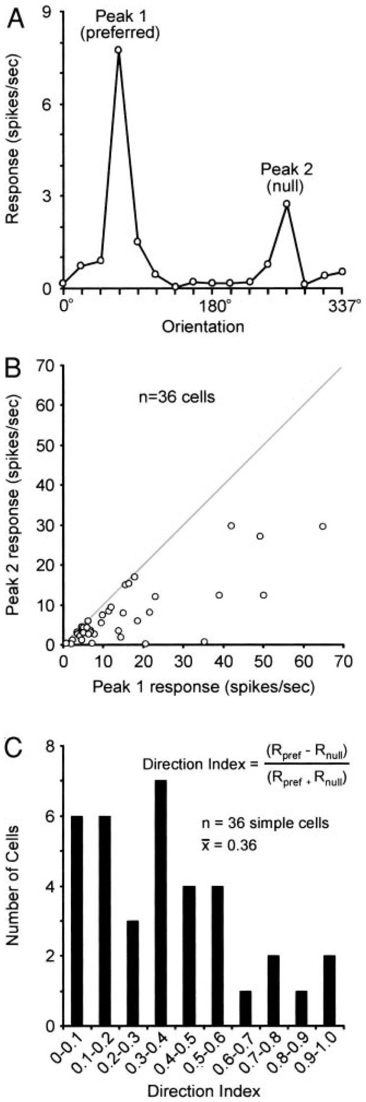
Direction selectivity of layer 4 neurons. A: peaks in orientation-tuning curves were used to assess the direction selectivity of individual neurons. B: scatter-plot showing the relationship between responses (peak 1, peak 2) to gratings moving in opposite directions. Points falling along the line of unit slope (gray) represent neurons with little or no difference in their response to gratings moving in opposite directions. Neurons below the line of unit slope represent neurons with varying degrees of direction selectivity. C: the direction index was calculated for individual neurons to quantify and compare direction selectivity among simple cells (mean: 0.36 ± 0.05).
Relationship between receptive-field structure and orientation selectivity
We used two types of stimuli to characterize the response properties of layer 4 neurons—white-noise stimuli and sinusoidal grating stimuli. As can be appreciated from the examples shown in Fig. 2, the long axis of a simple cell receptive field closely approximates that cell's preferred orientation for grating stimuli. To quantify this relationship, we used the white-noise receptive field map to model and simulate an orientation tuning curve (see METHODS) and compared the simulated tuning curve to the cell's actual tuning curve made using a drifting sine wave grating (Fig. 6). The relationship between the predicted preferred orientation and measured preferred orientation among our sample of simple cells is shown in Fig. 7A. For most cells, their was a high degree of correlation between the predicted preferred orientation and the measured preferred orientation (r2 = 0.85, P = 0.001). We also compared the bandwidth of orientation tuning from modeled and measured tuning curves by comparing the half-width of peaks at half-maximum response (Fig. 7B). The average ratio of measured half-width to predicted half-width was 1.9 (P < = 0.001). Thus the orientation tuning of most layer 4 simple cells is tighter than a linear model based on the cells' spatial receptive field would predict.
FIG. 6.

Demonstration of how orientation tuning curves were simulated from m-sequence maps. The 1st-order kernel response map from m-sequence white-noise simulation (A) was fitted with a Gabor filter (B). Responses were fitted for the time delay (t) that produced the maximal response. C: sine wave grating stimuli composed of the optimal spatial frequency and varying over orientation were convolved with the Gabor filters from B. After convolving the stimulus with the filter, the output was half-wave rectified and summed over space to yield a single response magnitude for each orientation. D: the modeled orientation tuning curve (—) is shown plotted along with the measured tuning curve using a drifting sine wave grating (normalized, - - -). The simulation allows us to compare the peak orientations for the gabor simulation (27°) and the drifting grating spike rate (22.5°) as well as the orientation half-width (35 and 20°, respectively).
FIG. 7.

Comparison of orientation tuning for linear model predictions and neuronal responses to drifting sine wave gratings. A: the optimal orientation (peak in the orientation tuning curve) is shown plotted for the neuronal responses elicited from drifting sine wave gratings vs. model simulations from the best fitting gabor filters to white-noise maps estimated from reverse correlation to m-sequence stimuli. There is a high degree of correlation between the estimates from the neuronal responses and the linear model predictions (r2 = 0.85, P < 0.001). B: estimates of orientation tuning bandwidth (half-width at half-height) for the drifting grating responses versus the Gabor filter simulations. On average, the linear model simulation predicts greater orientation tuning bandwidth than those estimated from the drifting gratings responses. The average bandwidth ratio, drifting grating response to simulation, is 1.9 (P < 0.001).
The extent to which a cell's receptive field is elongated can be expressed numerically as a ratio of its length versus width (aspect ratio). For each of the simple cells in this study, we fit the white-noise receptive field with a Gabor function and then estimated the aspect ratio of the receptive-field subregion that gave the strongest response (see METHODS). Aspect ratios among our sample of layer 4 simple cells ranged from ~1 to 4 with a mean of 2.45 and a median of 2.3 (Fig. 8). While our estimates of aspect ratio in layer 4 of the ferret are somewhat lower than those found in several studies of cat simple cells (Jones and Palmer 1987: range, 1.7-12; median, ~5; Gardner et al. 1999: range, 2-12; median, ~3.5; but see Pei et al. 1994: range, 1-4, mean, 1.7), the values we report are more consistent with studies that emphasized simple cells in layer 4 of cat visual cortex (Bullier et al. 1982: ~2; Martinez et al. 1999: mean, 2.3; Alonso et al. 2001: mean, 2.5).
FIG. 8.

Length-to-width aspect ratios for simple-cell receptive-field subunits. All estimates are based on m-sequence reverse correlation maps. The raw data were fitted with a Gabor function. The width of the subunits was estimated as the full width at 20% height of the dominant subunit from the fitted Gabors. Lengths were estimated as the full width at 20% height of the Gaussian envelope of the Gabor function. ↑, the population mean (2.45).
Finally, we examined the relationship between receptive-field shape and degree of orientation selectivity by comparing the aspect ratio of the strongest subregion to the half width of the primary peak in the orientation-tuning curve. We found that neurons with high aspect ratios tended to have narrower peaks (Fig. 9). In contrast, neurons with low aspect ratios displayed a broader range of half widths. However, there was not a significant correlation between orientation bandwidth and RF subunit aspect ratio (Fig. 9, r2 = 0.14). A similar relationship between aspect ratio and half width was recently reported in the cat (Gardner et al. 1999).
FIG. 9.

Orientation tuning half-width vs. receptive-field subunit aspect ratio. Comparison of the orientation tuning curve bandwidth (half-width at half-height) estimated from neuronal spike rates (drifting grating stimulation) with the receptive field subunit aspect ratio (length/width, for the dominant subunit) estimated from the m-sequence reverse correlation 1st-order maps. Although there is no significant correlation between the 2 estimates (r2 = 0.14), there is a tendency for neurons with higher aspect ratios to have lower peak half widths.
We also compared the orientation half-width to the number of subunits (data not shown). The Gabor filter fits to the white-noise maps were analyzed to determine the number of subunits. Subunits were counted if they produced responses that were >20% of the maximum response. On average, receptive fields with two subunits had orientation half-widths (⟨orientation half-width⟩ = 20.7) that were significantly greater (2 sample t-test P < 0.05) than receptive fields that had three subunits (⟨orientation half-width⟩ = 17.4).
DISCUSSION
We studied the visual responses of neurons in layer 4 of primary visual cortex in the adult ferret. Most neurons (84%) recorded from in layer 4 were orientation-selective simple cells. These neurons had elongated receptive fields with sub-regions that were either ON or OFF. We also encountered a smaller percentage (16%) of neurons in layer 4 that lacked orientation selectivity and had center/surround receptive fields. In the sections that follow, we compare the response properties of ferret layer 4 neurons with those in other species and consider the potential neural mechanisms underlying the responses of layer 4 neurons in the ferret.
Comparison with other species
Two types of receptive fields were found in our sample of ferret layer 4 neurons—simple and center/surround. While simple receptive fields have elongated and adjacent subregions that are either ON or OFF, center/surround receptive fields have circular centers (either ON or OFF) and opposing surrounds. The response properties of layer 4 neurons have arguably been studied most extensively in the cat. Like the ferret, most neurons in layer 4 of cat visual cortex are simple cells with elongated and adjacent subregions. Unlike the ferret, cat layer 4 also contains a small population of complex cells (Gilbert 1977; Hubel and Wiesel 1962; see also Henry et al. 1979)—a cell type not encountered in our sample of layer 4 ferret neurons. Although we attempted to include in our sample all neurons encountered during an electrode penetration across layer 4, it is always possible that our recordings were biased against complex cells. Similarly, because complex cells are only a small percentage (~5-30%) of the cells in layer 4 of the cat (Gilbert 1977; Hubel and Wiesel 1962; see also Henry et al. 1979), it is also possible that our sample size (n = 51) was not large enough to include complex cells.
The number of subregions present in a cat simple cell is typically two or three (occasionally 4) (Alonso et al. 2001; Jones and Palmer 1987; Kulikowski and Bishop 1981; Movshon et al. 1978; Mullickin et al. 1984; Reid et al. 1997). Similarly, we found that ferret simple cells typically have two or three subregions (see also McKay et al. 2001). Our results also show that aspect ratios (length vs. width) of layer 4 simple receptive fields are similar between ferret (mean 2.45) and cat (Bullier et al. 1982: ~2; Jones and Palmer 1987: median, ~5; Pei et al. 1994: mean, 1.7; Gardner et al. 1999: median, ~3.5; Martinez et al. 1999: ~2; Alonso et al. 2001: mean, 2.5). Thus many spatial properties of cat simple cells appear similar in the ferret.
The extent to which simple cells exist in layer 4 of other species is less clear. Simple cells are absent from layer 4 in the tree shrew and absent or occasionally encountered (depending on reports) in layer 4Cβ in the macaque monkey where neurons, in both species, have been shown to have center/surround receptive fields (Blasdel and Fitzpatrick 1984; Hubel and Wiesel 1968, 1977; Humphrey and Norton 1980; Lennie et al. 1990; Leventhal et al. 1995; Livingstone and Hubel 1984; Ringach et al. 2002). Neurons with center/surround receptive fields have also been described in layer 4Cα of the macaque monkey (Blasdel and Fitzpatrick 1984; Hubel and Wiesel 1968, 1977; Lennie et al. 1990; Livingstone and Hubel 1984); however, the majority of 4Cα neurons appear to have simple receptive fields (Blasdel and Fitzpatrick 1984; Bullier and Henry 1980; Hawken et al. 1988; Leventhal et al. 1995; Livingstone and Hubel 1984; Ringach et al. 2002). Based on the types of receptive fields present in layer 4C of the macaque monkey—primarily center/surround in 4Cβ, center/surround and simple in 4Cα—it could be argued that ferret layer 4 more closely resembles monkey 4Cα than monkey 4Cβ. This suggestion is consistent with the view that neurons in layer 4Cβ of the macaque monkey are members of a pathway involved with high spatial resolution and/or color vision (reviewed in Lee 1996; Livingstone and Hubel 1988; Schiller and Logothetis 1990; but see Lennie et al. 1991; Rodieck 1991)—a pathway not present in the ferret.
As with simple cells in cat and monkey, the simple cells that we recorded from in layer 4 of ferret visual cortex were selective for stimulus orientation. Orientation-tuning curves were made from neural responses to drifting sine-wave gratings presented at 16 different orientations. To quantify the tightness of peaks in these tuning curves, we measured peak half widths at half maximal response. Among our sample of simple cells, the average half width was 21.5 ± 1.2°. This value is remarkably similar to values for simple cells in the cat and monkey (~20°) (Gilbert 1977; Henry et al. 1974; Kato et al. 1978; Orban 1984; Schiller et al. 1976). Given the similarity in bandwidth for orientation tuning across species, it is tempting to speculate that tuning bandwidth is optimized for a common computational task, and/or there is a conservation of mechanisms responsible for establishing orientation selectivity.
Two previous studies that specifically examined orientation selectivity among layer 4 neurons in the ferret (Chapman and Stryker 1993; Weliky and Katz 1997) both found layer 4 neurons to be more broadly tuned than we report in the current study. Three possible causes for the discrepancy are the type or amount of anesthetic used, the nature of the stimulus employed, and the sampling procedure. With respect to anesthesia, the two previous studies used thiopental sodium (Chapman et al. 1991) and halothane (Weliky and Katz 1997), whereas isoflurane was used in the current study. It is of course not possible to assess any variability between the exact anesthetic states of the animals used in different experiments or to know whether such variability might underlie the observed difference in layer 4 orientation tuning. Regarding visual stimuli, both of the previous studies assayed orientation selectivity using bar stimuli. In contrast, the current study used sinusoidal gratings of optimal spatial frequency. A major difference between grating and bar stimuli is that gratings excite (or inhibit) all of the subregions (both ON and OFF) of a simple cell receptive field simultaneously. Whether or not this greater increase in net excitation (or inhibition) underlies the differences reported for orientation selectivity remains to be determined. Still, it is worth noting that past studies comparing measurements (or predictions) of receptive-field size have found differences that do depend on whether bar or grating stimuli are used (Andrews and Pollen 1979; Glezer et al. 1980; Kulikowski and Bishop 1981; Tadmor and Tolhurst 1989). Finally, in the two previous studies, single units were recorded every 80 μm (Chapman et al. 1991) or 150 μm (Weliky and Katz 1997) to avoid sampling bias, whereas in the current study, units that responded vigorously to white-noise stimuli were purposefully isolated.
Potential neural mechanisms underlying layer 4 responses
Because this study represents the first description of simple cells in layer 4 of ferret visual cortex, the mechanisms responsible for establishing the spatial organization of ON and OFF subregions in the simple cell receptive field remain to be determined. If ferret circuitry proves to be similar to that in the cat, then it seems likely that ferret simple cells are constructed by a precise organization of connections from both thalamic and intracortical sources. Studies in the cat have shown that LGN cells provide monosynaptic input to simple cells only when their receptive fields are spatially overlapped with a simple cell receptive field and match the sign (ON or OFF) of the overlapped subregion (Alonso et al. 2001; Reid and Alonso 1995; Tanaka 1983; Usrey et al. 2000). There is, however, a major difference between the organization of geniculate inputs to layer 4 in cat and ferret. In the cat, ON and OFF geniculate axons terminate in an overlapping fashion in layer 4 (Alonso et al. 2001; Reid and Alonso 1995; Usrey et al. 2000). In contrast, ON and OFF geniculate axons in the ferret terminate in separate patches of layer 4 (Zahs and Stryker 1988; see also McConnell and LeVay 1984). Based on this segregation, we expected to find patches of layer 4 cells whose responses were dominated by either ON or OFF responses. Instead, we found that many ferret simple cells had receptive fields with similarly strong ON and OFF subregions. Moreover, while we often encountered sequential simple cells along an electrode penetration that had a similar sign (ON or OFF) to their strongest subregion, we also encountered sequential simple cells with opposite signs to their strongest subregion. Based on these results, we would argue that simple cells in layer 4 of ferret visual cortex have access to both the ON and OFF streams. Whether or not this access is direct from the LGN, or indirect from intracortical sources, remains to be determined.
The spatial organization of geniculate inputs to simple cells may also play a role in establishing the orientation-selective responses of layer 4 simple cells. Studies examining the spatial extent of geniculate inputs to single cortical columns in the ferret (Chapman et al. 1991) or single layer 4 neurons in the cat (Alonso et al. 2001; Reid and Alonso 1995; Usrey et al. 2000) have shown that the spatial location of geniculate receptive fields fall along a line that generally corresponds to the preferred orientation of the cortical column or individual cell. A more direct test of the role that geniculate inputs might play in establishing orientation selectivity was performed by Ferster and colleagues. These studies compared the orientation selectivity of cat layer 4 neurons in the presence and absence of intracortical input and found that geniculate input alone could generate layer 4 responses that matched the orientation preference of a cell when the cortical circuit was intact (Chung and Ferster 1998; Ferster et al. 1996). Although the extent to which orientation selectivity is determined by thalamic input is still a matter of debate (reviewed in Das 1996; Reid and Alonso 1996; Sompolinsky and Shapley 1997), it is clear that thalamic input alone cannot account for all features of simple cell responses. For instance, if thalamic input alone were to entirely determine orientation selectivity, then one would predict that simple cells with longer receptive fields (high aspect ratios) would have orientation-tuning curves with smaller peak half widths compared with simple cells with shorter receptive fields (low aspect ratios). Consistent with results from the cat (Gardner et al. 1999; but see Lampl et al. 2001), we found that whereas simple cells with high aspect ratios indeed have peak half widths that cluster toward low values, simple cells with low aspect ratios have peak half widths that are distributed along the entire range of high to low values (Fig. 9). This finding would suggest that simple cells with low aspect ratios and small peak half widths must rely on intracortical mechanisms to tighten their orientation tuning. Moreover, contrast invariance of orientation tuning—a property shared by all simple cells thus far studied—almost certainly relies on intra-cortical sources of input to layer 4 neurons (Sclar and Freeman 1982; Skottun et al. 1987; Usrey and Alitto 2002; reviewed in Ferster and Miller 2000; Sompolinsky and Shapley 1997).
Despite the unusual arrangement of segregated ON- and OFF-center geniculocortical inputs to ferret layer 4 (Zahs and Stryker 1988) and despite previous reports that many ferret layer 4 cells are poorly tuned for orientation selectivity (Chapman et al. 1991; Weliky and Katz 1997), we have found that ferret layer 4 cells are very similar to those seen in cat and monkey. This suggests that both the function and the mechanisms of the first processing stage in visual cortex may be well conserved across species.
Acknowledgments
Expert technical assistance was provided by P. Barruel, F. Farzin, A. Haines, and J. Major.
This work was supported by National Eye Institute Grants EY-13588, EY-11369, and EY-12576, the McKnight Foundation, the Esther A. and Joseph Klingenstein Fund, and the Alfred P. Sloan Foundation.
Footnotes
The costs of publication of this article were defrayed in part by the payment of page charges. The article must therefore be hereby marked “advertisement” in accordance with 18 U.S.C. Section 1734 solely to indicate this fact.
REFERENCES
- Alitto HJ, Collins OA, Usrey WM. The influence of corticothalamic feedback on the responses of neurons in the lateral geniculate nucleus. Soc Neurosci Abstr. 2002:658.1b. [Google Scholar]
- Alonso J-M, Usrey WM, Reid RC. Rules of connectivity between geniculate cells and simple cells in cat primary visual cortex. J Neurosci. 2001;21:4002–4015. doi: 10.1523/JNEUROSCI.21-11-04002.2001. [DOI] [PMC free article] [PubMed] [Google Scholar]
- Andrews BW, Pollen DA. Relationship between spatial-frequency selectivity and receptive-field profile of simple cells. J Physiol (Lond) 1979;287:163–176. doi: 10.1113/jphysiol.1979.sp012652. [DOI] [PMC free article] [PubMed] [Google Scholar]
- Azouz R, Gray CM, Nowak LG, McCormick DA. Physiological properties of inhibitory interneurons in cat striate cortex. Cereb Cortex. 1997;7:534–545. doi: 10.1093/cercor/7.6.534. [DOI] [PubMed] [Google Scholar]
- Blasdel GG, Fitzpatrick D. Physiological organization of layer 4 in macaque striate cortex. J Neurosci. 1984;4:880–895. doi: 10.1523/JNEUROSCI.04-03-00880.1984. [DOI] [PMC free article] [PubMed] [Google Scholar]
- Bullier J, Henry GH. Laminar distribution of first-order neurons and afferent terminals in cat striate cortex. J Neurophysiol. 1979;42:1271–1281. doi: 10.1152/jn.1979.42.5.1271. [DOI] [PubMed] [Google Scholar]
- Bullier J, Henry GH. Ordinal position and afferent input of neurons in monkey striate cortex. J Comp Neurol. 1980;193:913–935. doi: 10.1002/cne.901930407. [DOI] [PubMed] [Google Scholar]
- Bullier J, Mustari MJ, Henry GH. Receptive-field transformations between LGN neurons and S-cells of cat-striate cortex. J Neurophysiol. 1982;47:417–438. doi: 10.1152/jn.1982.47.3.417. [DOI] [PubMed] [Google Scholar]
- Chapman B, Godecke I. No ON/OFF maps in supragranular layers of ferret visual cortex. J Neurophysiol. 2002;88:2163–2166. doi: 10.1152/jn.2002.88.4.2163. [DOI] [PMC free article] [PubMed] [Google Scholar]
- Chapman B, Godecke I, Bonhoeffer T. Development of orientation preference in the mammalian visual cortex. J Neurobiol. 1999;41:18–24. doi: 10.1002/(sici)1097-4695(199910)41:1<18::aid-neu4>3.0.co;2-v. [DOI] [PMC free article] [PubMed] [Google Scholar]
- Chapman B, Stryker MP. Development of orientation selectivity in ferret visual cortex and effects of deprivation. J Neurosci. 1993;13:5251–5262. doi: 10.1523/JNEUROSCI.13-12-05251.1993. [DOI] [PMC free article] [PubMed] [Google Scholar]
- Chapman B, Zahs KR, Stryker MP. Relation of cortical cell orientation selectivity to alignment of receptive fields of the geniculocortical afferents that arborize within a single orientation column in ferret visual cortex. J Neurosci. 1991;11:1347–1358. doi: 10.1523/JNEUROSCI.11-05-01347.1991. [DOI] [PMC free article] [PubMed] [Google Scholar]
- Chung S, Ferster D. Strength and orientation tuning of the thalamic input to simple cells revealed by electrically evoked cortical suppression. Neuron. 1998;20:1177–1189. doi: 10.1016/s0896-6273(00)80498-5. [DOI] [PubMed] [Google Scholar]
- Citron MC, Kroeker JP, McCann GD. Nonlinear interactions in ganglion cell receptive fields. J Neurophysiol. 1981;46:1161–1176. doi: 10.1152/jn.1981.46.6.1161. [DOI] [PubMed] [Google Scholar]
- Cleland BG, Dubin MW, Levick WR. Sustained and transient neurones in the cat's retina and lateral geniculate nucleus. J Physiol (Lond) 1971;217:473–496. doi: 10.1113/jphysiol.1971.sp009581. [DOI] [PMC free article] [PubMed] [Google Scholar]
- Das A. Orientation in visual cortex: a simple mechanism emerges. Neuron. 1996;16:477–480. doi: 10.1016/s0896-6273(00)80067-7. [DOI] [PubMed] [Google Scholar]
- Erwin E, Miller KD. Correlation-based development of ocularly matched orientation and ocular dominance maps: determination of required input activities. J Neurosci. 1998;18:9870–9895. doi: 10.1523/JNEUROSCI.18-23-09870.1998. [DOI] [PMC free article] [PubMed] [Google Scholar]
- Ferster D, Chung S, Wheat H. Orientation selectivity of thalamic input to simple cells of cat visual cortex. Nature. 1996;380:249–252. doi: 10.1038/380249a0. [DOI] [PubMed] [Google Scholar]
- Ferster D, Miller KD. Neural mechanisms of orientation selectivity in the visual cortex. Annu Rev Neurosci. 2000;23:441–471. doi: 10.1146/annurev.neuro.23.1.441. [DOI] [PubMed] [Google Scholar]
- Gardner JL, Anzai A, Ohzawa I, Freeman RD. Linear and nonlinear contributions to orientation tuning of simple cells in the cat's striate cortex. Vis Neurosci. 1999;16:1115–1121. doi: 10.1017/s0952523899166112. [DOI] [PubMed] [Google Scholar]
- Gielen CCAM, van Gisbergen JAM, Vendrik AJH. Reconstruction of cone-system contributions to responses of color-opponent neurones in monkey lateral geniculate. Biol Cybern. 1982;44:211–221. doi: 10.1007/BF00344277. [DOI] [PubMed] [Google Scholar]
- Gilbert CD. Laminar differences in receptive field properties of cells in cat primary visual cortex. J Physiol (Lond) 1977;268:391–421. doi: 10.1113/jphysiol.1977.sp011863. [DOI] [PMC free article] [PubMed] [Google Scholar]
- Glezer VD, Tscherbach TA, Fauselman VE, Bondarko VM. Linear and nonlinear properties of simple and complex receptive fields in area 17 of the cat visual cortex. Biol Cybern. 1980;37:195–208. doi: 10.1007/BF00337038. [DOI] [PubMed] [Google Scholar]
- Hawken MJ, Parker AJ. Contrast sensitivity and orientation selectivity in lamina IV of the striate cortex of Old World monkeys. Exp Brain Res. 1984;54:367–372. doi: 10.1007/BF00236238. [DOI] [PubMed] [Google Scholar]
- Hawken MJ, Parker AJ, Lund JS. Laminar organization and contrast sensitivity o f direction-selective cells in the striate cortex of the Old World monkey. J Neurosci. 1988;8:3541–3548. doi: 10.1523/JNEUROSCI.08-10-03541.1988. [DOI] [PMC free article] [PubMed] [Google Scholar]
- Hendrickson AE, Wilson JR, Ogren MP. The neuroanatomical organization of pathways between the dorsal lateral geniculate nucleus and visual cortex in Old World and New World primates. J Comp Neurol. 1978;182:123–136. doi: 10.1002/cne.901820108. [DOI] [PubMed] [Google Scholar]
- Henry GH, Dreher B, Bishop PO. Orientation specificity of cells in cat striate cortex. J Neurophysiol. 1974:1394–1409. doi: 10.1152/jn.1974.37.6.1394. [DOI] [PubMed] [Google Scholar]
- Henry GH, Harvey AR, Lund JS. The afferent connections and laminar distribution of cells in the cat striate cortex. J Comp Neurol. 1979;187:725–744. doi: 10.1002/cne.901870406. [DOI] [PubMed] [Google Scholar]
- Hubel DH, Wiesel TN. Integrative action in the cat's lateral geniculate body. J Physiol (Lond) 1961;155:385–398. doi: 10.1113/jphysiol.1961.sp006635. [DOI] [PMC free article] [PubMed] [Google Scholar]
- Hubel DH, Wiesel TN. Receptive fields, binocular interaction and functional architecture in the cat's visual cortex. J Physiol (Lond) 1962;160:106–154. doi: 10.1113/jphysiol.1962.sp006837. [DOI] [PMC free article] [PubMed] [Google Scholar]
- Hubel DH, Wiesel TN. Receptive fields and functional architecture of monkey striate cortex. J Physiol (Lond) 1968;195:215–243. doi: 10.1113/jphysiol.1968.sp008455. [DOI] [PMC free article] [PubMed] [Google Scholar]
- Hubel DH, Wiesel TN. Laminar and columnar distribution of geniculocortical fibers in the macaque monkey. J Comp Neurol. 1972;146:421–450. doi: 10.1002/cne.901460402. [DOI] [PubMed] [Google Scholar]
- Hubel DH, Wiesel TN. Functional architecture of macaque monkey visual cortex. Proc R Soc Lond B Biol Sci. 1977;198:1–59. doi: 10.1098/rspb.1977.0085. [DOI] [PubMed] [Google Scholar]
- Humphrey AL, Norton TT. Topographic organization of the orientation column system in the striate cortex of the tree shrew (Tupaia glis). I. Microelectrode recording. J Comp Neurol. 1980;192:531–547. doi: 10.1002/cne.901920311. [DOI] [PubMed] [Google Scholar]
- Ikeda H, Wright MJ. Receptive field organization of “sustained” and “transient” retinal ganglion cells which subserve different function roles. J Physiol (Lond) 1972;227:769–800. doi: 10.1113/jphysiol.1972.sp010058. [DOI] [PMC free article] [PubMed] [Google Scholar]
- Jones JP, Palmer LA. The two-dimensional spatial structure of simple receptive fields in cat striate cortex. J Neurophysiol. 1987;58:1187–1211. doi: 10.1152/jn.1987.58.6.1187. [DOI] [PubMed] [Google Scholar]
- Kato H, Bishop PO, Orban GA. Hypercomplex and simple/complex cell classifications in cat striate cortex. J Neurophysiol. 1978;41:1071–1095. doi: 10.1152/jn.1978.41.5.1071. [DOI] [PubMed] [Google Scholar]
- Katz LC, Shatz CJ. Synaptic activity and the construction of cortical circuits. Science. 1996;274:1133–1138. doi: 10.1126/science.274.5290.1133. [DOI] [PubMed] [Google Scholar]
- Kelly JP, Van Essen DC. Cell structure and function in the visual cortex of the cat. J Physiol (Lond) 1974;238:515–547. doi: 10.1113/jphysiol.1974.sp010541. [DOI] [PMC free article] [PubMed] [Google Scholar]
- Kretz R, Rager G, Norton TT. Laminar organization of ON and OFF regions and ocular dominance in the tree shrew (Tupaia balangeri) J Comp Neurol. 1986;251:135–145. doi: 10.1002/cne.902510110. [DOI] [PubMed] [Google Scholar]
- Kulikowski JJ, Bishop PO. Linear analysis of the responses of simple cells in the cat visual cortex. Exp Brain Res. 1981;44:386–400. doi: 10.1007/BF00238831. [DOI] [PubMed] [Google Scholar]
- Lampl I, Anderson JS, Gillespie DC, Ferster D. Prediction of orientation selectivity from receptive field architecture in simple cells of cat visual cortex. Neuron. 2001;30:263–274. doi: 10.1016/s0896-6273(01)00278-1. [DOI] [PubMed] [Google Scholar]
- Law MI, Zahs KR, Stryker MP. Organization of primary visual cortex (area 17) in the ferret. J Comp Neurol. 1988;278:157–180. doi: 10.1002/cne.902780202. [DOI] [PubMed] [Google Scholar]
- Lee BB. Receptive field structure in the primate retina. J Comp Neurol. 1996;36:631–644. doi: 10.1016/0042-6989(95)00167-0. [DOI] [PubMed] [Google Scholar]
- Lennie P, Haake PW, Williams DR. The design of chromatically opponent receptive fields. In: Landy MS, Movshon JA, editors. Computational Models of Visual Processing. MIT Press; Cambridge, MA: 1991. pp. 71–82. [Google Scholar]
- Lennie P, Krauskopf J, Sclar G. Chromatic mechanisms in striate cortex of macaque. J Neurosci. 1990;10:649–669. doi: 10.1523/JNEUROSCI.10-02-00649.1990. [DOI] [PMC free article] [PubMed] [Google Scholar]
- LeVay S, McConnell SK, Luskin MB. Functional organization of primary visual cortex in the mink (Mustela vison), and a comparison with the cat. J Comp Neurol. 1987;257:422–441. doi: 10.1002/cne.902570310. [DOI] [PubMed] [Google Scholar]
- Leventhal AG, Thompson KG, Liu D, Zhou Y, Ault SJ. Concomitant sensitivity to orientation, direction, and color of cells in layers 2, 3, and 4 of monkey striate cortex. J Neurosci. 1995;15:1808–1818. doi: 10.1523/JNEUROSCI.15-03-01808.1995. [DOI] [PMC free article] [PubMed] [Google Scholar]
- Livingstone MS, Hubel DH. Anatomy and physiology of a color system in the primate visual cortex. J Neurosci. 1984;4:309–356. doi: 10.1523/JNEUROSCI.04-01-00309.1984. [DOI] [PMC free article] [PubMed] [Google Scholar]
- Livingstone MS, Hubel DH. Segregation of form, color, movement, and depth: anatomy, physiology, and perception. Science. 1988;240:740–749. doi: 10.1126/science.3283936. [DOI] [PubMed] [Google Scholar]
- Martinez LM, Reid RC, Alonso JM, Hirsch JA. The synaptic structure of the simple receptive field. Soc Neurosci Abstr. 1999;25:1048. [Google Scholar]
- McConnell SK, LeVay S. Segregation of on- and off-center afferents in mink visual cortex. Proc Natl Acad Sci USA. 1984;81:1590–1593. doi: 10.1073/pnas.81.5.1590. [DOI] [PMC free article] [PubMed] [Google Scholar]
- McCormick DA, Connors BW, Lighthall JW, Prince DA. Comparative electrophysiology of pyramidal and sparsely spiny stellate neurons of the neocortex. J Neurophysiol. 1985;54:782–806. doi: 10.1152/jn.1985.54.4.782. [DOI] [PubMed] [Google Scholar]
- McKay SM, Smyth D, Akerman CJ, Thompson ID. Changing receptive fields during development in ferret primary visual cortex. Soc Neurosci Abstr. 2001;27:475.13. [Google Scholar]
- Miller KD. A model for the development of simple cell receptive fields and the ordered arrangement of orientation columns through activity-dependent competition between ON- and OFF-center inputs. J Neurosci. 1994;14:409–441. doi: 10.1523/JNEUROSCI.14-01-00409.1994. [DOI] [PMC free article] [PubMed] [Google Scholar]
- Miller KD, Erwin E, Kayser A. Is the development of orientation selectivity instructed by activity? J Neurobiol. 1999;41:44–57. doi: 10.1002/(sici)1097-4695(199910)41:1<44::aid-neu7>3.0.co;2-v. [DOI] [PubMed] [Google Scholar]
- Mooney R, Penn AA, Gallego R, Shatz CJ. Thalamic relay of spontaneous retinal activity prior to vision. Neuron. 1996;17:863–874. doi: 10.1016/s0896-6273(00)80218-4. [DOI] [PubMed] [Google Scholar]
- Movshon JA, Thompson ID, Tolhurst DJ. Spatial summation in the receptive fields of simple cells in the cat's striate cortex. J Physiol (Lond) 1978;283:53–77. doi: 10.1113/jphysiol.1978.sp012488. [DOI] [PMC free article] [PubMed] [Google Scholar]
- Mullikin WH, Jones JP, Palmer LA. Periodic simple cells in cat area 17. J Neurophysiol. 1984;52:372–387. doi: 10.1152/jn.1984.52.2.372. [DOI] [PubMed] [Google Scholar]
- Orban GA. Neuronal Operations in the Visual Cortex. Springer Verlag; Berlin: 1984. [Google Scholar]
- Pei X, Vidyasagar TR, Volgushev M, Creutzfeldt OD. Receptive field analysis and orientation selectivity of postsynaptic potentials of simple cells in cat visual cortex. J Neurosci. 1994;14:7130–7140. doi: 10.1523/JNEUROSCI.14-11-07130.1994. [DOI] [PMC free article] [PubMed] [Google Scholar]
- Reid RC, Alonso JM. Specificity of monosynaptic connections from thalamus to visual cortex. Nature. 1995;378:281–284. doi: 10.1038/378281a0. [DOI] [PubMed] [Google Scholar]
- Reid RC, Alonso JM. The processing and encoding of information in the visual cortex. Curr Opin Neurobiol. 1996;6:475–480. doi: 10.1016/s0959-4388(96)80052-3. [DOI] [PubMed] [Google Scholar]
- Reid RC, Victor JD, Shapley RM. The use of m-sequences in the analysis of visual neurons: linear receptive field properties. Vis Neurosci. 1997;14:1015–1027. doi: 10.1017/s0952523800011743. [DOI] [PubMed] [Google Scholar]
- Ringach DL, Shapley RM, Hawken MJ. Orientation selectivity in macaque V1: diversity and laminar dependence. J Neurosci. 2002;22:5639–5651. doi: 10.1523/JNEUROSCI.22-13-05639.2002. [DOI] [PMC free article] [PubMed] [Google Scholar]
- Rockland KS. Anatomical organization of primary visual cortex (area 17) in the ferret. J Comp Neurol. 1985;241:225–236. doi: 10.1002/cne.902410209. [DOI] [PubMed] [Google Scholar]
- Rodieck RW. Which cells code for color? In: Valberg A, Lee BB, editors. From Pigments to Perception. Plenum; New York: 1991. pp. 83–93. [Google Scholar]
- Schiller PH, Finlay BL, Volman SF. Quantitative studies of single-cell properties in monkey striate cortex. II. Orientation specificity and ocular dominance. J Neurophysiol. 1976;39:1320–1333. doi: 10.1152/jn.1976.39.6.1320. [DOI] [PubMed] [Google Scholar]
- Schiller PH, Logothetis NK. The color-opponent and broadband channels of the primate visual system. Trends Neurosci. 1990;13:392–398. doi: 10.1016/0166-2236(90)90117-s. [DOI] [PubMed] [Google Scholar]
- Sclar G, Freeman RD. Orientation selectivity in the cat's striate cortex is invariant with stimulus contrast. Exp Brain Res. 1982;46:457–461. doi: 10.1007/BF00238641. [DOI] [PubMed] [Google Scholar]
- Skottun BC, Bradley A, Sclar G, Ohzawa I, Freeman RD. The effects of contrast on visual orientation and spatial frequency discrimination: a comparison of single cells and behavior. J Neurophysiol. 1987;57:773–786. doi: 10.1152/jn.1987.57.3.773. [DOI] [PubMed] [Google Scholar]
- Sompolinsky H, Shapley R. New perspectives on the mechanisms for orientation selectivity. Curr Opin Neurobiol. 1997;7:514–522. doi: 10.1016/s0959-4388(97)80031-1. [DOI] [PubMed] [Google Scholar]
- Sutter EE. A practical non-stochastic approach to nonlinear time-domain analysis. In: Marmarelis V, editor. Advanced Methods of Physiological Systems Modeling. vol. 1. University of Southern California; Los Angeles, CA: 1987. pp. 303–315. 1987. [Google Scholar]
- Sutter EE. A deterministic approach to nonlinear systems analysis. In: Pinter R, Nabet B, editors. Nonlinear Vision: Determination of Neural Receptive Fields, Function and Networks. CRC; Cleveland, OH: 1992. pp. 171–220. [Google Scholar]
- Tadmor Y, Tolhurst DJ. The effect of threshold on the relationship between the receptive-field profile and the spatial frequency tuning curve in simple cells of the cat's striate cortex. Visual Neurosci. 1989;3:445–454. doi: 10.1017/s0952523800005940. [DOI] [PubMed] [Google Scholar]
- Tanaka K. Cross-correlation analysis of geniculostriate neuronal relationships in cats. J Neurophysiol. 1983;49:1303–1318. doi: 10.1152/jn.1983.49.6.1303. [DOI] [PubMed] [Google Scholar]
- Tavazoie SF, Reid RC. Diverse receptive fields in the lateral geniculate nucleus during thalamocortical development. Nat Neurosci. 2000;3:608–616. doi: 10.1038/75786. [DOI] [PubMed] [Google Scholar]
- Usrey WM, Alitto HJ. The effect of stimulus contrast on orientation and temporal fequency tuning of neurons in ferret primary visual cortex. Soc Neurosci Abstr. 2002:456.8. [Google Scholar]
- Usrey WM, Alonso J-M, Reid RC. Synaptic interactions between thalamic inputs to simple cells in cat visual cortex. J Neurosci. 2000;20:5461–5467. doi: 10.1523/JNEUROSCI.20-14-05461.2000. [DOI] [PMC free article] [PubMed] [Google Scholar]
- Usrey WM, Reid RC. Synchronous activity in the visual system. Annu Rev Physiol. 1999;61:435–456. doi: 10.1146/annurev.physiol.61.1.435. [DOI] [PubMed] [Google Scholar]
- Usrey WM, Reid RC. Visual physiology of the lateral geniculate nucleus in two species of New World monkey: Saimiri sciureus and Aotus trivirgatis. J Physiol (Lond) 2000;523:755–769. doi: 10.1111/j.1469-7793.2000.00755.x. [DOI] [PMC free article] [PubMed] [Google Scholar]
- Usrey WM, Reppas JB, Reid RC. Specificity and strength of retinogeniculate connections. J Neurophysiol. 1999;82:3527–3540. doi: 10.1152/jn.1999.82.6.3527. [DOI] [PubMed] [Google Scholar]
- Weliky M, Katz LC. Disruption of orientation tuning in visual cortex by artificially correlated neuronal activity. Nature. 1997;386:680–685. doi: 10.1038/386680a0. [DOI] [PubMed] [Google Scholar]
- Zahs KR, Stryker MP. Segregation of ON and OFF afferents to ferret visual cortex. J Neurophysiol. 1988;59:1410–1429. doi: 10.1152/jn.1988.59.5.1410. [DOI] [PubMed] [Google Scholar]