Fast multipole methods for particle dynamics

Abstract

The growth of simulations of particle systems has been aided by advances in computer speed and algorithms. The adoption of O(N) algorithms to solve N-body simulation problems has been less rapid due to the fact that such scaling was only competitive for relatively large N. Our work seeks to find algorithmic modifications and practical implementations for intermediate values of N in typical use for molecular simulations. This article reviews fast multipole techniques for calculation of electrostatic interactions in molecular systems. The basic mathematics behind fast summations applied to long ranged forces is presented along with advanced techniques for accelerating the solution, including our most recent developments. The computational efficiency of the new methods facilitates both simulations of large systems as well as longer and therefore more realistic simulations of smaller systems.

1. Introduction

Particle simulations are a practical way of studying average or ensemble properties as well as the dynamics of a variety of systems, from galaxies to molecular fluids. While very efficient algorithms exist for systems where physics dictates finite or short ranged interactions between particles, [17,54,55,59] many systems require different physics. The problem of long ranged forces, that is forces where the potential goes like r^−p for 0 < p ≤ 3, requires procedures to force convergence. While enforcing a finite range or cutoffs have been used, they change the physics which can have unpredictable effects [16]. The use of lattice sums and reaction fields, especially for p = 1 in three dimensions obtains the required convergence. These techniques have algorithms which do better than the naive N² algorithms obtaining, in favorable cases, O(N log N). However the scaling to large numbers of processors for relatively small values of N remains a problem for such algorithms. The growth of computer speed has made such algorithms practical for systems of O(10 K) particles but has inhibited the total number of configurations possible to visit.

The wide spread adoption of O(N) algorithms, via fast summation techniques, to solve N-body simulation problems has been less rapid due to the fact that such scaling was only competitive for relatively large N. In order to get linear scaling for small to intermediate systems it is necessary to consider the way the mapping of the algorithm onto the architecture affects the various bottlenecks in the computation.

In Section 2 of this paper, we include a brief historical overview of traditional methods for calculation of electrostatic interactions and fast hierarchical methods. Section 3 presents basic multipole equations. We then consider in some detail each of the major operations in the algorithm from a computational point of view. Sections 4, 5, 6 and 7 present the basic transformations associated with the multipole coefficients. In addition, Section 7 discusses various proposed acceleration methods for the translation operation in detail. Section 8 summarizes the overall scheme common to the entire fast multipole method (FMM). Section 9 focuses on implementation of periodic boundary conditions within FMM. Section 10 reviews performance analysis and is devoted to performance improvements essential for efficient implementation of FMM. Section 11 addresses important implementation issues. Finally, Section 12 comments on aspects that are essential to the parallelization of FMM.

2. Particle methods

As short ranged potentials are essentially a solved problem [44,56–58,60,61] we will concentrate on the long ranged problem. Other authors have considered the problem for 1 and 2 dimensional systems [74,75]. Since the functional form (power law) of the solution to Poison's equation depends on dimension we will restrict our interest to systems in three dimensions where Coulomb's law takes its familiar form for the potential of 1/r where r is the distance between particles. This is similar to the gravitational case except that gravity only has attractions whereas electrostatics has both attractions and repulsions. By the definitions given above Coulomb's law produces configurational integrals which naively diverge for many body systems. Physically, the charges screen each other producing a renormalized force law avoiding the divergence. Computationally, the sums or integrals must be forced to converge under most circumstances of interest using convergence factors or techniques which are also common in most analytic treatments such as even Fourier transforming a Coulomb potential. The use of lattice sums are a popular method for obtaining convergence although not the only physically motivated method available [52].

2.1 Ewald methods

In 1921, Ewald [35] proposed his lattice summation technique for calculating interactions between a set of particles and all their infinite periodic images solely to address the problem of the conditional convergence of the direct sum. Although the original Ewald method was not initially designed for computational performance, later on it gave rise to a number of fast algorithms which exceed in performance the direct N² sum of a nonperiodic system [79]. State of the art are the methods referred to as Fourier-based Ewald summation methods. Representative of this group is the particle–particle particle–mesh method, PPPM or P³M [52,64], and the particle–mesh Ewald method, PME [23,34], both based on the algorithm developed by Hockney and Eastwood [29,45]. In these methods, the electrostatic field is expressed as a sum of two components: a short range force and the long range force that is left, where the former is calculated using a cutoff and the latter is calculated by extending a regular grid over the domain and solving Poisson's equation on the grid using the FFT to accelerate the solution. These methods reduce the complexity of Ewald summation to O(N log N), are well understood and highly popular in the molecular dynamics community. The works by Toukmaji and Board [83] and Sagui and Darden [68] offer excellent overviews of Ewald summation techniques. The articles [15,22,24,25] also provide valuable insights.

2.2 Hierarchical methods

The hierarchical methods are based on the idea that one particle can interact with a group of other particles by approximating their combined effect rather than interacting with every one of them, provided the group is far enough from the particle. This is essentially a tree structure based method which is common to all fast summation techniques. The milestones on the road to FMM were the papers by Appel [7] and Barnes and Hut [8]. The FMM was first designed by Greengard and Rokhlin, who used spherical harmonics to developed all the mathematical apparatus required by a truly O(N) algorithm [38,40]. An interesting approach was also proposed by Anderson [6]. Warren and Salmon did important work on data structures required by efficient hierarchical methods [69,70,86–89]. Although being an O(N) solution to the grand challenge problem [1] and being qualified as one of top ten most important algorithmic discoveries of the twentieth century [11,28] FMM has not yet enjoyed high popularity. The computation complexity of FMM has been questioned [4] and it has been pointed out that there can be a significant constant coefficients hidden under the big O notation [10]. It was even claimed that in comparison to the P³M method “FMM can only become faster at some unphysical size N > 10⁶⁰” [62].

It is, however, hard to argue with FMM's algorithmic beauty. Thus work on the scaling of the coefficients is a natural avenue for research. In fact FMM has steadily gained in practical performance since its conception and has become a competitor for Ewald-style methods with certain approximate schemes [26,27]. We believe that its full potential is yet to be discovered. To make it practical one must achieve both linear scaling as well as a reasonable coefficients and offsets at particle numbers used regularly in molecular simulations O(10 K).

3. Multipole representation of electrostatic field

All hierarchical N-body algorithms are based on the idea of evaluating combined effect of a set of distant particles instead of treating them individually. In the FMM the electrostatic field has a dual representation. It is described by multipole expansion and a so-called local or Taylor expansion, both expressed using spherical harmonics. Spherical harmonics ${\text{Y}}_n^m(\alpha ,\beta )$ are functions of two coordinates α, β (usually angles) on the surface of a sphere, orthogonal for different n and m and normalized so that their integrated square over the sphere is unity:

$$Y_n^{-m}(\alpha ,\beta )=\sqrt{\frac{2n+1}{4\pi }\frac{(n-m)!}{(n+m)!}}{\text{e}}^{\text{im}\beta }{\text{P}}_n^m(cos\alpha ).$$ (3.1)

In FMM however the normalization factor $\sqrt{(2n+1)/4\pi }$ is commonly omitted. The ${\text{P}}_n^m(x)$ in equation (3.1) are associated Legendre polynomials, which can be defined in terms of the ordinary Legendre polynomials P_n(x) by the Rodrigues formula

$${\text{P}}_n^m(x)={(-1)}^m{(1-x^2)}^{m/2}\frac{{\text{d}}^m}{\text{d}{x}^m}{P}_n(x).$$ (3.2)

In appendix A we give a simple method for calculating Legendre polynomials.

In the formulation by Greengard and Rokhlin [20,38,40,42] the multipole expansion for a set of N charges q₁, q₂, …, q_N with spherical coordinates $\overrightarrow{r_1}=({\rho }_1,{\alpha }_1,{\beta }_1),\overrightarrow{r_2}=({\rho }_2,{\alpha }_2,{\beta }_2),\dots ,\overrightarrow{r_N}=({\rho }_N,{\alpha }_N,{\beta }_N)$ located inside a sphere S centered at the origin is defined by the formula

$${\text{M}}_n^m=\sum _{i=1}^N{q}_i{\rho }_i^n{Y}_n^{-m}({\alpha }_i,\beta i),$$ (3.3)

where $Y_n^{-m}(\alpha ,\beta )$ are spherical harmonics of degree n and order m defined with a non unit square integrated normalization as

$$Y_n^{-m}(\alpha ,\beta )=\sqrt{\frac{(n-|m|)!}{(n+|m|)!}}{\text{e}}^{im\beta }{P}_n^{|m|}(cos\alpha ).$$ (3.4)

For any point r⃗ = (ρ, α, β) located outside the sphere S containing all the charges the potential due to these charges is given by the formula

$$\Phi (\overrightarrow{r})=\sum _{n=0}^{\infty }\sum _{m=-n}^n\frac{{\text{M}}_n^m}{{\rho }^{n+1}}{\text{Y}}_n^m(\alpha ,\beta ).$$ (3.5)

Figure 1 shows the shape of the field associated with different multipole moments.

Figure 1.

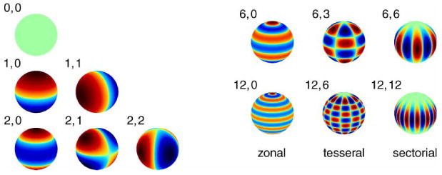
Multipole moments.

The local expansion for a set of N charges q₁, q₂, …, q_N with spherical coordinates $\overrightarrow{r_1}=({\rho }_1,{\alpha }_1,{\beta }_1),\overrightarrow{r_2}=({\rho }_2,{\alpha }_2,{\beta }_2),\dots ,\overrightarrow{r_N}=({\rho }_N,{\alpha }_N,{\beta }_N)$ located outside a sphere S centered at the origin is defined by the formula

$${\text{L}}_n^m=\sum _{i=1}^N{q}_i\frac{Y_n^{-m}({\alpha }_i,{\beta }_i)}{{\rho }_i^{n+1}},$$ (3.6)

For any point r⃗ = (ρ, α, β) located inside the sphere S the potential due to these charges is given by the formula

$$\Phi (\overrightarrow{r})=\sum _{n=0}^{\infty }\sum _{m=-n}^n{\text{L}}_n^m{\rho }^n{\text{Y}}_n^m(\alpha ,\beta ).$$ (3.7)

It is important to stress here that the potential expressed by the multipole expansion (3.5) can only be evaluated outside of the sphere containing all the charges. At the same time the potential expressed by local expansion (3.7) can only be evaluated inside the sphere not containing any charges contributing to the local expansion. The sums in equations (3.5) and (3.7) will not converge if these conditions are violated. The physical explanation is that we can accurately approximate the combined effect of a set of charges only if they are close to one another and far from the point of approximation.

For computer implementations of FMM it is more convenient to use a simplified form of the multipole expansion in solid harmonics introduced by Wang and LeSar [85]. Here we will follow the notation by Elliott [32]. In this formulation the multipole and local expansions and the potential are expressed using ${\text{F}}_n^m(\overrightarrow{r})$ and ${\text{G}}_n^m(\overrightarrow{r})$ functions, which correspondingly define regular and irregular solid harmonics:

$${\text{F}}_n^m(\overrightarrow{r})=\frac{{(-1)}^{n-m}{\rho }^n}{(n+m)!}{\text{e}}^{im\beta }{\text{P}}_n^m(cos\alpha ),$$ (3.8)

$${\text{G}}_n^m(\overrightarrow{r})=\frac{{(-1)}^{n-m}(n-m)!}{{\rho }^{n+1}}{\text{e}}^{im\beta }{\text{P}}_n^m(cos\alpha ).$$ (3.9)

$${\text{M}}_n^m=\sum _{i=1}^N{q}_i{F}_n^{\ast m}(-\overrightarrow{r_i}),$$ (3.10)

$${\text{L}}_n^m=\sum _{i=1}^N{q}_i{\text{G}}_n^m(-\overrightarrow{r_i}),$$ (3.11)

$$\Phi (\overrightarrow{r})=\sum _{n=0}^{\infty }\sum _{m=-n}^n{\text{M}}_n^m{\text{G}}_n^m(\overrightarrow{r}),$$ (3.12)

$$\Phi (\overrightarrow{r})=\sum _{n=0}^{\infty }\sum _{m=-n}^n{\text{L}}_n^m{F}_n^{\ast m}(\overrightarrow{r}),$$ (3.13)

Most importantly these equations allow for a simple formulation of the translation operators which will be introduced in §7. Also see appendix D for equations for calculating the force (the negative gradient of the potential) from the multipole and local expansions.

In computer code the range of n in the multipole equations is truncated to a finite number of p terms, depending on convergence requirements. Usually p ranges from 8 to 30 and for molecular dynamics the value of 16 seems to be a convenient compromise between numerical accuracy and computational cost. Figure 2 shows convergence of the field representation with increasing order of expansion p.

Figure 2.

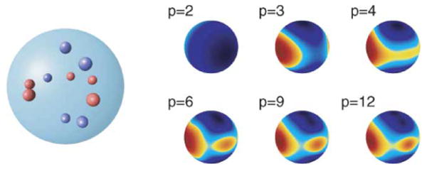
Convergence of field representation with order of expansion p.

Normally one would have to store and manipulate the coefficients of the multipole and local expansions, ${\text{M}}_n^m$ and ${\text{L}}_n^m$, and the ${\text{G}}_n^m(\overrightarrow{r})$ and ${\text{F}}_n^m(\overrightarrow{r})$ functions for n ∈ [0, p − 1] and m′ ∈ [−n, n]. However due to the following symmetries:

$$F_n^{-m}(\overrightarrow{r})={(-1)}^m{F}_n^{\ast m}(\overrightarrow{r}),$$ (3.14)

$$G_n^{-m}(\overrightarrow{r})={(-1)}^m{G}_n^{\ast m}(\overrightarrow{r}),$$ (3.15)

$$M_n^{-m}={(-1)}^m{M}_n^{\ast m},$$ (3.16)

$$L_n^{-m}={(-1)}^m{L}_n^{\ast m},$$ (3.17)

we may use only positive values of m saving storage and computation time. Thus, in optimized implementations it is essential to implement these expansions and functions in the form of triangular matrices.

4. Scaling of multipole coefficients

The ρⁿ term in the multipole expansion coefficients ${\text{M}}_n^m$ (equation (3.8)) and the 1/ρⁿ⁺¹ term in the ${\text{G}}_n^m(\overrightarrow{r})$ function coefficients (equation (3.9)), may cause the coefficients to vary by orders of magnitude which may cause numerical problems during summation and the translation operation discussed in §7. It is not a concern if translations are implemented as a O(p⁴) convolution/correlation type of operation. However, some of the extensive optimizations designed to speed up translations (less than O(p⁴)) can suffer in precision due to roundoff errors. In order to avoid these problems the multipole expansion coefficients of a cubic box of dimension d are scaled to the coefficients of a unit size box before translations:

$${\stackrel{\sim }{M}}_n^m=\frac{{\text{M}}_n^m}{d^{n+1}},$$ (4.1)

and then after translations the local expansion coefficients are scaled back to coefficients of the box of original size:

$${\stackrel{\sim }{L}}_n^m=\frac{{\text{L}}_n^m}{d^n}.$$ (4.2)

As we can see from equations (4.1) and (4.2) scaling is an order O(p²) operation. Scaling can only improve numerical results of FMM and in practice costs almost nothing in the computation time. It is also convenient for constant pressure algorithms.

5. Rotation of multipole coefficients

A class of acceleration methods for FMM takes advantage of the fact that the computational cost of translations, in particular the multipole to local translation discussed in §7, can be reduced when the translation is performed along the Z-axis (along the vector described by α = 0). One such method, presented by White and Head-Gordon, reduces the computational complexity of translation to O(p³) [91]. The most recent one, introduced by Greengard and Rokhlin, further reduces the computation complexity to O(p²) [42] (§7.2.3). The idea is to rotate the coordinate system in such a way that the z coefficient of the translation vector is dominant, perform the translation with a reduced computational cost and then rotate the system back to its original orientation. As a result all translation vectors are divided into six groups corresponding to six faces of the cube. The scheme is referred to as a “rotate-shift-rotate translation”. By the same token such methods require the ability of rotating the multipole and local expansion coefficients by ±π/2 and ±π about the coordinate system axis.

The rotation of spherical harmonics also relates to the properties of angular momentum in quantum mechanics and has been well investigated [9,30,84]. We start with the fact that in general an arbitrary rotation can be accomplished in three steps via Euler rotations, and can be characterized by the three Euler angles. However the problem simplifies greatly in the context of FMM. We notice that all the required rotations can be achieved by a combination of at most two rotations about the axis of the coordinate system. All necessary rotations can be performed either by rotating about the Y-axis or by first rotations about the Z-axis and then about the Y-axis. Overall only the following operations are needed: rotations by ±π/2 and ±π about the Y-axis and rotations by ±π/2 about the Z-axis. The translations for the six groups of vectors can then be represented as the following combinations of rotations and a translation along the Z-axis:

$${\text{Trans}}_{+Z}={\text{Trans}}_{+Z},$$ (5.1)

$${\text{Trans}}_{+X}={\text{Rot}}_Y(-\pi /2){\text{Trans}}_{+Z}{\text{Rot}}_Y(\pi /2),$$ (5.2)

$${\text{Trans}}_{-X}={\text{Rot}}_Y(\pi /2){\text{Trans}}_{+Z}{\text{Rot}}_Y(-\pi /2),$$ (5.3)

$$\begin{array}{l}{\text{Trans}}_{+Y}={\text{Rot}}_Z(-\pi /2){\text{Rot}}_Y(-\pi /2){\text{Trans}}_{+Z}\\ \times {\text{Rot}}_Y(\pi /2){\text{Rot}}_Z(\pi /2),\end{array}$$ (5.4)

$$\begin{array}{l}{\text{Trans}}_{-Y}={\text{Rot}}_Z(-\pi /2){\text{Rot}}_Y(\pi /2){\text{Trans}}_{+Z}\\ \times {\text{Rot}}_Y(-\pi /2){\text{Rot}}_Z(\pi /2),\end{array}$$ (5.5)

$${\text{Trans}}_{-Z}={\text{Rot}}_Y(-\pi ){\text{Trans}}_{+Z}{\text{Rot}}_Y(\pi ).$$ (5.6)

A rotation by an angle α about the Z-axis only changes the phase of the moments and is trivial to implement using the formulas:

$$\begin{array}{cc}{\stackrel{\sim }{M}}_n^m={\text{M}}_n^m{\text{e}}^{\text{im}\alpha },& {\stackrel{\sim }{L}}_n^m={\text{L}}_n^m{\text{e}}^{\text{im}\alpha },\end{array}$$ (5.7)

which for α = ±π/2 translates in the implementation to operations as simple as exchanges of real and imaginary parts of complex numbers and changes of sign. Also trivial to implement is the rotation by the angle β = ±π about the Y-axis using the following relation between the original coefficients and the rotated coefficients:

$$\begin{array}{cc}{\stackrel{\sim }{M}}_n^m={(-1)}^n{M}_n^{\ast m},& {\stackrel{\sim }{L}}_n^m={(-1)}^n{L}_n^{\ast m}.\end{array}$$ (5.8)

The only non-trivial rotation is the rotation by β = ±π/2 about the Y-axis. These rotations can be performed using Wigner rotation matrices $R_n^{m,m^{\prime }}(\beta )$. The rotation matrices are block diagonal mixing m values of the spherical harmonics with a given n:

$$\begin{array}{c}{\stackrel{\sim }{M}}_n^{m^{\prime }}=\sum _{m=-n}^n{R}_n^{m,m^{\prime }}(\beta ){\text{M}}_n^m,\\ {\stackrel{\sim }{L}}_n^{m^{\prime }}=\sum _{m=-n}^n{R}_n^{m,m^{\prime }}(\beta ){\text{L}}_n^m.\end{array}$$ (5.9)

A variety of methods to compute the coefficients $R_n^{m,m^{\prime }}(\beta )$ have been developed. See [9,30,84] for a more complete discussion. In appendix B we give formulae for calculating Wigner matrix coefficients that we found straightforward to implement.

The rotations about the Z-axis and the rotation by π about the Y-axis are all O(p²) complexity operations that require just one pass through the expansion coefficients. The rotation by ±π/2 about the Y-axis is much more expensive O(p³) operation that involves expansion coefficients and Wigner matrix coefficients. Unfortunately all translations, except for translations along the Z-axis, require the costly rotation involving the Wigner matrix. However in serial FMM the rotations are performed a lot less frequently than the translation along the Z-axis and their practical overhead is minimal.

6. Mirror reflection about the XY plane

One last transformation that is handy in FMM is the mirror reflection about the XY plane. We can see that if for the vector r⃗ in equations (3.8) and (3.9) we change α to π − α, then the new expansion will be related to the original expansion by:

$$\begin{array}{cc}{\stackrel{\sim }{M}}_n^m={(-1)}^{n+m}{M}_n^{\ast m},& {\stackrel{\sim }{L}}_n^m={(-1)}^{n+m}{L}_n^{\ast m}.\end{array}$$ (6.1)

Another way to come to the same conclusion is by combining rotation by π about the Z-axis and rotation by π about the Y-axis by conjoining equations (5.7) and (5.8). Just as for the two above mentioned rotations, the mirror reflection is O(p²) in complexity and requires just one pass over expansion coefficients. The impact of this relation is further discussed in §10.4.

7. Translation of multipole coefficients

Translations are the most important operations in the FMM algorithm. The FMM algorithm can be implemented in its basic form without the use of either scaling or rotation. However translations are in the core of the algorithm and the quality of their implementation is essential to performance.

7.1 Multipole to multipole and local to local translations

The translation of the center of a multipole expansion by a vector r⃗_M2M is referred to as multipole to multipole or M2M translation. The translation of the center of a local expansion by a vector r⃗_L2L is referred to as local to local or L2L translation. M2M and L2L translations have a very simple form in Elliott's notation:

$$M_{n^{\prime }}^{m^{\prime }}=\sum _{n=0}^{\infty }\sum _{m=-n}^n{\text{M}}_n^m{F}_{n^{\prime }-n}^{\ast m^{\prime }-m}({\overrightarrow{r}}_{\text{M}2\text{M}}),$$ (7.1)

$$L_{n^{\prime }}^{m^{\prime }}=\sum _{n=0}^{\infty }\sum _{m=-n}^n{\text{L}}_n^m{F}_{n-n^{\prime }}^{\ast m-m^{\prime }}({\overrightarrow{r}}_{\text{L}2\text{L}}).$$ (7.2)

According to equations (7.1) and (7.2) these are convolution type operations of O(p⁴) complexity. It is important to efficiently evaluate these formulas, but there is little reason to try to improve on their computation complexity since the computation time in FMM will always be dominated by the multipole to local translations described in the following section.

7.2 Multipole to local translation

The most important operation in FMM is the multipole to local or M2L translation by a vector r⃗_M2L which converts a multipole expansion to a local expansion with a new center. A multipole expansion cannot be evaluated within the sphere containing the constituent charges and it cannot be shifted by M2L translation to a point within this sphere. It can only be M2L shifted to a point outside the sphere where the resulting local expansion can be evaluated. The expression for M2L translation has similarly simple form to the M2M and L2L translations mentioned in previous section:

$$L_{n^{\prime }}^{m^{\prime }}=\sum _{n=0}^{\infty }\sum _{m=-n}^n{\text{M}}_n^m{G}_{n^{\prime }+n}^{m^{\prime }+m}({\overrightarrow{r}}_{\text{M}2\text{L}}).$$ (7.3)

It also has the same O(p⁴) computation complexity. However unlike the other translations, M2L translation is the most crucial to performance of FMM and the subject of extensive efforts to lower its computation complexity are described in following sections.

7.2.1 Fourier form

Since the M2L translation is a convolution, the most obvious improvement is to replace it with a product in Fourier space. This was proposed early by Greengard and Rokhlin [41] and later perfected by Elliott and Board [33]. In practice this method is implemented by placing the multipole expansion ${\text{M}}_n^m$ and the transfer matrix ${\text{G}}_n^m({\overrightarrow{r}}_{\text{M}2\text{L}})$ in rectangular arrays of size 2p × p, performing the Fourier transform on the matrices, performing elementwise product of the matrices, performing inverse Fourier transform of the product and extracting the local expansion coefficients from the resulting matrix. The transition from circular convolution to linear convolution requires zero padding in the n direction resulting in array length of 2p. However due to the triangular nature of the convolved matrices no zero padding in the m direction is necessary. Also we do not explicitly represent the coefficients for negative values of m, but they have to be implicitly handled by the Fourier transform routine. Although it may not be the most elegant way of performing Fourier transforms, in this case the desired efficiency can be achieved by performing one dimensional fast Fourier transform (FFT) by rows and then by columns. In this case the row FFT has to be modified to handle the implicit coefficients for negative m. On the other hand, we can save time by not performing FFT on the empty rows introduced by zero padding. The column FFT is thus a regular stride FFT routine. Figure 3 shows the idea of fast Fourier acceleration of translation. As already mentioned in §4 the FFT acceleration technique suffers from numerical instability due to the ρⁿ term in the multipole expansion coefficients ${\text{M}}_n^m$ (equation (3.8)) and the 1/ρⁿ⁺¹ term in the ${\text{G}}_n^m(\overrightarrow{r})$ function coefficients (equation (3.9)), which may cause the coefficients to vary by many orders of magnitude. To alleviate this problem the coefficients need to be scaled for a unit box before the FFT method can be applied. Since scaling is a low overhead operation this does not cause any performance problems. Scaling will only guarantee numerical accuracy for expansion sizes up to p = 16, which happens to be satisfactory for most molecular dynamics simulations. In most cases higher accuracy would exceed the accuracy of time integrators. If higher accuracy is required other acceleration techniques have to be used. Two alternatives are discussed in the following sections. There is however a performance price to pay for all other acceleration methods and the method described in this section is the fastest M2L speedup mechanism currently in use often providing an order of magnitude improvement in computation time over the standard method with accuracy suitable for molecular dynamics simulations. This method is also compatible with parallelization.

Figure 3.

The fast Fourier transform acceleration of translation.

7.2.2 Fourier form with block decomposition

Elliott and Board addressed the problem of numerical instability of the FFT acceleration method for bigger expansion sizes [33]. At the same time, their method eliminates the need for scaling altogether. The method is similar to the one described in previous section except that the matrices are decomposed into blocks of four rows each. Each block is individually zero padded with four empty rows and Fourier transformed. The multiplication in Fourier space is replaced with convolution of the resulting blocks. Following is the inverse Fourier transform of the blocks and extraction of the resulting local expansion. The method is about four times faster than the standard method, but at the same time about twice slower than the Fourier method without block decomposition. It does not increase storage requirements however and just as the former method it is very suitable for parallelization.

7.2.3 Exponential (plane wave) form

Later, Greengard and Rokhlin devised another speedup mechanism where in order to perform fast translations they switch from an expansion in spherical harmonics to expansion in plane waves, also referred to as exponential expansion [42]. The paper by Hrycak and Rokhlin [46] describes the adaptive two dimensional version of the algorithm and the paper by Cheng et al. [20] describes the adaptive three dimensional version of the algorithm. We assume here multipole equations in the formulation by Greengard and Rokhlin (equations (3.3)–(3.7)). (Transition from Elliott–Board representation to Greengard–Rokhlin representation is straightforward.)

The exponential expansion for a set of N charges q₁, q₂, …, q_N with Cartesian coordinates (x₁, y₁, z₁), (x₂, y₂, z₂), …, (x_N, y_N, z_N) located inside a cubic box of unit size centered at the origin is defined by the formula:

$$W(k,j)=\frac{{\omega }_k}{M_k}\sum _{l=1}^N{q}_l{\text{e}}^{{\lambda }_k{z}_l}{\text{e}}^{-i{\lambda }_k(x_{l}cos{\alpha }_{jk}+y_{l}sin{\alpha }_{jk})},$$ (7.4)

where k ∈ [1, s], j ∈ [1, M_k], α_jk = (2πj/M_k) and the triplets {λ_k, ω_k, M_k} have to be properly chosen for a given s. The value of s equal to p in spherical harmonics should result in similar accuracy. Table A1 in the appendix provides the values for s = 8.

For a point X with Cartesian coordinates (x, y, z) satisfying the conditions

$$\begin{array}{cc}1\le z\le 4,& 0\le \sqrt{x^2+y^2}\le 4\sqrt{2}.\end{array}$$ (7.5)

The approximate potential due to these charges is given by the formula

$$\Phi (X)\approx \sum _{k=1}^s\sum _{j=1}^{M_k}W(k,j){\text{e}}^{-{\lambda }_{k}z}{\text{e}}^{i{\lambda }_k(xcos{\alpha }_{jk}+ysin{\alpha }_{jk})}.$$ (7.6)

In FMM however the exponential form is only used as an intermediate representation of electrostatic field for the duration of the translation operation. The exponential expansion is never calculated using charges and their positions nor is the potential calculated from the exponential expansion. Expansion in plane waves W(k, j) is calculated based on multipole expansion in spherical harmonics ${\text{O}}_n^m$ (following Greengard and Rokhlin's notation ${\text{O}}_n^m$ is used instead of ${\text{M}}_n^m$ to distinguish it from M_k). This can be done using the formula

$$\begin{array}{l}W(k,j)=\frac{{\omega }_k}{M_k}\sum _{m=-p}^p{(-i)}^{\left|m\right|}{\text{e}}^{im{\alpha }_{jk}}\\ \times \sum _{n=\left|m\right|}^p\frac{{({\lambda }_k)}^n}{\sqrt{(n-m)!(n+m)!}}{\text{O}}_n^m.\end{array}$$ (7.7)

Then the exponential expansion can be translated by a vector X⃗ with Cartesian coordinates (x, y, z) satisfying the condition (7.5) using the formula

$$V(k,j)=W(k,j){\text{e}}^{-{\lambda }_{k}z}{\text{e}}^{i{\lambda }_k(xcos{\alpha }_{jk}+ysin{\alpha }_{jk})}$$ (7.8)

and finally the shifted expansion can be translated to local expansion in spherical harmonics by the formula

$${\text{L}}_n^m=\frac{{(-i)}^{\left|m\right|}}{\sqrt{(n-m)!(n+m)!}}\sum _{k=1}^s{(-{\lambda }_k)}^n\sum _{j=1}^{M_k}V(k,j){\text{e}}^{\text{im}{\alpha }_{jk}}.$$ (7.9)

Before performing a translation using the plane wave representation we need to scale the multipole coefficients to coefficients of a unit size box (§4), then rotate the coordinate system to point the translation vector in the positive z direction such that it satisfies the conditions (7.5) (§5) and then convert the expansion in spherical harmonics to the expansion in plane waves (equation (7.7)). At this point the translation can be performed as a fast O(p²) operation (equation (7.8)). When it is done we need to translate the result back to the local expansion in spherical harmonics (equation (7.9)), rotate it back to the orientation of the original coordinate system and scale it back to the original size. As in the case of the Fourier technique the speedup comes from the fact that the fast formula (7.8) can be evaluated many more times than the accompanying scalings, rotations and conversions from spherical harmonics to plane waves. Figure 4 shows the idea of plane wave acceleration of translation.

Figure 4.

The plane wave acceleration of translation.

Although the formula (7.7) may suggest at first glance O(p⁴) complexity of the operation, in fact is can be implemented as O(p³) operation. First we can calculate quantities F_km defined by the formula

$$F_{km}=\sum _{n=\left|m\right|}^p\frac{{({\lambda }_k)}^n}{\sqrt{(n-m)!(n+m)!}}{\text{O}}_n^m$$ (7.10)

and then we can calculate the coefficients W(k, j) by the formula

$$W(k,j)=\frac{{\omega }_k}{M_k}\sum _{m=-p}^p{(-i)}^{\left|m\right|}{\text{e}}^{\text{im}{\alpha }_{jk}}{F}_{km}.$$ (7.11)

The same applies to the operation described by the formula (7.9). Unfortunately, the transition from spherical harmonics to plane waves described by the above formulas still remains a costly operation.

8. Putting it all together

In common practice today, the FMM algorithm is available in two main variants, as a nonadaptive algorithm suitable for fairly uniform charge distributions and as an adaptive algorithm suitable for highly nonuniform charge distributions. We first focus on the nonadaptive algorithm and then comment on its adaptive derivative.

8.1 Nonadaptive FMM

The FMM algorithm starts by subdividing the three dimensional simulation box into eight smaller boxes (octants) each of which is then again subdivided into eight yet smaller boxes and the process goes on recursively until desired level of subdivision in achieved. The cells are organized into a perfect octal tree where each node corresponds to a cell. The entire simulation box corresponds to the root node. Each node, except for the root node, has exactly one parent. Each node, except for the leaf nodes, has exactly eight children. The leaf nodes correspond to the finest level of spatial decomposition. Levels are numbered starting from number 0 for the level containing the root node, successively growing going down the tree. When this decomposition is done the cells on the finest level house the coordinates for the particles subject to the electrostatic field calculation. Then the algorithm proceeds in the following steps:

1. Multipole Expansion Evaluation: Each leaf cell calculates its multipole expansion based on positions and charges of particles contained in that cell according to equation (3.10).

2. Upward Pass: Multipole expansions are propagated up the tree. First each leaf cell shifts its multipole expansion to the one of its corners which is the center of its parent cell by means of multipole to multipole, or M2M, translation according to equation (7.1). The process continues level by level until the root cell aggregates expansions of all its eight children.

3. Multipole to Local Phase: Each cell on each level of the decomposition accumulates electrostatic information from cells which belong to its multipole neighborhood. In the classic formulation two cells on the same level of decomposition are multipole neighbors if they are situated at least two cells apart from each other and at the same time their parents are not multipole neighbors. As a result, the multipole neighborhood for a cell has more-less the shape of a hollow cube with the cell in its center. In this step each cell acquires information from its multipole neighbors. The parent of a cell acquires information about the region beyond it and the children of a cell acquire information about the hollow space inside it. The information acquisition is performed by shifting the multipole expansion of each neighbor to the center of a given cell and converting it to a local expansion by the means of multipole to local or M2L translation according to equation (7.3). The speedup mechanisms of §7.2 can be applied here.

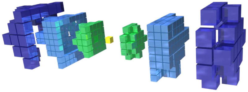
4. Downward Pass: Going from the root level down, each cell shifts its local expansion, accumulated in the previous step, to the centers of its eight children which accumulate and include this information with their own local expansion acquired in the previous step. This shift is performed by the means of the local to local, or L2L, translation according to equation (7.2). This process proceeds recursively downward in a waterfall manner. After this step is finished each leaf cell possesses a local expansion which reflects electrostatic field in the multipole neighborhood of the cell and all the space extending beyond it and does not include the contribution from the hollow region directly outside the cell. Figure 5 shows steps 2, 3 and 4 of the multipole calculations.

5. Local Expansion Evaluation: From the local expansion gathered in the previous two steps each leaf cell calculates the contribution to the potential and force on each of the particles contained in the cell according to equations (3.13) and (D.2).

6. Direct Particle to Particle Calculations: Each leaf cell accumulates for each particle the contribution to the force from the particles enclosed in the hollow space directly outside the cell which was omitted in the multipole calculations. This is performed by directly calculating all pairwise interactions between particles in this region using Coulomb's Law

   $$\overrightarrow{F}=q_1{q}_2\frac{\overrightarrow{r_1}-\overrightarrow{r_2}}{{|\overrightarrow{r_1}-\overrightarrow{r_2}|}^3},$$ (8.1)

   and, at least in theory, could be subject to taking advantage of Newton's Third Law, which cuts the number of computations by half. This may not be worth the communications cost in some implementations depending on architecture.

Figure 5.

Upward pass, M2L phase and downward pass.

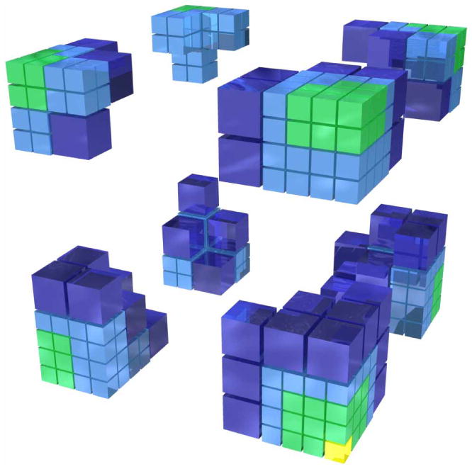
Figure 6 shows one of many possible shapes of direct and multipole interaction zones. The figure also depicts the idea of spherically shaped interaction regions discussed in detail in §10.1 and superblocks discussed in §10.2.

Figure 6.

Interaction zones: direct (green), multipole (blue); with superblocks in dark blue in online version.

The algorithm in the above formulation is a little different from the classic formulation [38,40] where steps 3 and 4 would be merged together and referred to as the downward pass. In this case, the multipole to local translations would be performed level by level, passing the local expansions downwards after processing each level. Although equivalent in serial implementation, such approach creates a huge bottleneck in parallel implementations where the computations associated with higher levels block computations on lower levels. The real benefit of the acceleration techniques discussed in §7.2 stems from the fact that the accompanying operations such scalings, rotations, FFTs, etc. can be factored outside of step 3, so that in step 3 only fast (O(p²)) operations take place. The computations associated with periodic boundary conditions, discussed in the following section, rely on the results of step 2 and are in turn required by the computations of step 4, so they can take place anywhere between those steps.

8.2 Adaptive FMM

The fundamental difference between the nonadaptive FMM and the adaptive FMM is that in the latter we do not use the same number of levels for all parts of the computational box. For strongly nonuniform particle distributions that would result in a large number of empty boxes at lower levels of the decomposition. Instead the recursive procedure continues to subdivide boxes only until they contain the number of particles that is greater that some fixed integer number. Although being a simple concept, the adaptiveness complicates the serial FMM algorithm substantially and yet more complicates its parallel implementation. At the same time in molecular dynamics, especially in simulations of liquids and even biomolecules in liquid, highly nonuniform distributions are uncommon and there would be little justification for the overhead associated with the adaptive FMM algorithm. For the same reasons the main competitors of FMM like P³M or PME use regular meshes with absolutely no notion of adaptation to nonuniform distributions. On the other hand adaptive FMM may be a powerful tool in areas where the distributions are highly nonuniform, like for gas-surface interactions and the astrophysical case of stellar dynamics.

There is a significant difference however for astrophysical (gravitational) applications. In molecular dynamics positive and negative charges cancel each other out and the monopole moment is small forcing more terms in the multipole expansion to achieve a desired level of precision. In stellar dynamics, where mass is always positive, the monopole term is large and low order approximations are sufficient. By the same token there is little reason for full-blown FMM with complex acceleration mechanism. For more details on the adaptive FMM the reader is referred to literature [18,20,38].

9. Periodic boundary conditions

In molecular dynamics, the system to be investigated is most often a small sample (O(10 K – 10 M) particles) of a bulk system (O(10²³). Edges produce correlations not representative of the bulk and so the use of some form of periodic boundary conditions are often appropriate to suppress effects of inappropriate boundaries [83]. However the first hierarchical N-body algorithms were introduced for the purpose of calculating gravitational forces in astrophysical simulations, were periodic boundary conditions did not exist [8]. Those algorithm were designed to speed up the naive N² method calculating all pairwise interactions in a nonperiodic set of particles. The FMM was originally conceived with provisions for PBCs in two dimensions [38]. But both in 2D and 3D periodic boundary conditions are a natural extension of the FMM introducing very little computational overhead and, as noted by Schmidt and Lee [71], actually simplifying the algorithm. Moreover they yet further simplify load balancing in parallel implementations of FMM [48].

The two most prominent methods incorporating periodic boundary conditions into FMM in three dimensions are the method by Schmidt and Lee [71,72] and the method by Lambert et al. [49]. Both approaches are based on the same basic observation that the periodic images have the same multipole expansion about their centers as the main box and they can readily be shifted to the center of the main box. Also, since all the expansions are the same, they factor out of the sum over all images. All the translation matrices can be accumulated into one transformation matrix. This matrix can then be applied to the multipole expansion of the main box to produce the local expansion of all periodic images. Most of work required by this step can be done during an initialization phase. The work required during simulation step is negligible and in parallel implementations can be assigned to one particular processor without causing any load imbalance. An important observation here is that the nearest neighbors of the main box cannot be treated in this manner because they are still subject to the separation criterion of the fast multipole algorithm. The empty space has to be filled out and this is where the simplifying effect of periodic boundary conditions takes place. In the nonperiodic systems, boxes near the faces of the cube have no neighboring boxes outside the cube and their interaction lists are thus truncated on the domain borders. With periodic boundary conditions, all boxes, both in the direct part and the multipole part, are treated exactly the same regardless of their position in the cube or their level in the octal tree. The “missing” boxes are replaced with periodic images appropriately for each level. These images are referred to as innermost cells. This produces the wraparound effect of periodic boundary conditions (figure 7). Practically, all the overhead of PBC in FMM comes from the introduction of the innermost cells. In parallel implementations the wraparound effect of the innermost cells results in much denser communication matrix with a clearly apparent antidiagonal. This is, of course, a sign of very poor locality in communications.

Figure 7.

Interaction zones for a corner cell with wraparound effect of periodic boundary conditions.

9.1 Infinite PBCs—Ewald method

Schmidt and Lee [71] have proposed a method for calculating the transformation matrix for infinite periodic boundary conditions based on the Ewald summation or lattice sum approach [83]. In order to shift the periodic images of the main box to its center the values of ${\rho }^{-(n+1)}{\text{e}}^{\text{jm}\beta }{\text{P}}_n^m(cos\alpha )$ in equation (3.9) are replaced by sum of the values corresponding to all the periodic images. The infinite sum is calculated using the Ewald method and then the contribution of the nearest cells (26 in this case) is explicitly subtracted. The method is equivalent to finding a solution to Poisson's equation for the field from charges in a periodic system. One can picture taking a finite number of replicas and surrounding the set of images by a vacuum with dielectric constant ε = 1 or ε = ∞. One then takes the limit as the number of replicas goes to infinity [3,71].

Thus, we have a straightforward solution, elegantly combining the fast multiple method with Ewald summation. Although Shimada et al. [73] point out some typographic errors in the paper, the follow-up paper by Schmidt and Lee [72] generalizes the method to noncubic lattices and gives more a detailed presentation of the mathematical apparatus. The readers who would like deeper explanation of this approach from mathematical perspective are also referred to the paper by Singer [75]. The papers by Challacombe et al. [19] and Figueirido et al. [36] also offer some interesting insights into these techniques. The most recent developments are reported by Amisaki [5].

9.2 Arbitrarily large finite PBCs—macroscopic expansion

Lambert and Board [49] have proposed a method for calculating the transformation matrix for finite yet arbitrarily large periodic boundary conditions based on hierarchical multilevel approach referred to as the macroscopic expansion (ME). In the nonperiodic FMM, upward propagation of multipole expansions stops at the main cell. In ME the process continues further up. The multipole expansions of the main box and 26 of its adjacent periodic replicas are combined into an aggregate higher level cell and the process goes recursively up to k levels. Since all the multipole expansions of the replicas on a given level are the same, they factor out of the sum and can be accumulated into one multipole to multipole transformation matrix for each level. Then at each level the cell centered at the main box accumulates contributions from its well separated periodic images using multipole to local translations and then conceptually passes the resulting local translation to the lower level. Since actually the levels are centered at the same point, there is no need for any local to local translations and the contributions from all levels are simply added to the local expansion of the main box. Here again all multipole expansions on a given level are the same, factor out of the sum and can be accumulated into one multipole to local transformation matrix for each level. When the process is finished the downward propagation of local expansions proceeds like in the nonperiodic FMM case. As a result the overhead of ME is k multipole to multipole transformations performed going in the upward direction and k multipole to local transformations performed going in the downward direction. In practice k between 4 and 6 approximates the infinite Ewald sum with high accuracy. Lambert and Board's method is, in our view, the most natural way of implementing PBCs in FMM. It does not introduce any new equations to the algorithm and can be coded with very little programming effort.

10. More performance improvements

There are two main parameters in FMM which can be used to trade accuracy for performance. One is the size of multipole expansions p used. The second one is the minimum separation of cells being considered multipole neighbors. Both larger values of p and larger separation, which results in a larger multipole and direct neighborhood, give higher accuracy and larger computation time. They can also be balanced against each other; we can keep the same accuracy by lowering one when increasing the other. In the original formulation by Greengard and Rokhlin a multipole neighbor of a cell is required to be separated from the cell by at least one other cell. In this case the size of the multipole interaction region is 189 cells and the worst case error was proved to be less than (0.75)^p. The plane wave acceleration technique by Greengard and Rokhlin [20,42] also relies on this separation criterion. However, those authors also suggested that multipole neighbors could be separated by at least two intervening cells of the same size in which case the size of the multipole interaction region is 875 cells and the worst case error is proved to be less than (0.4)^p.

Interesting work on the error analysis for FMM was also done by White and Head-Gordon [90], Elliott and Board [31] and Solvason and Petersen [80]. In following sections we discuss performance improvements which will decrease the size of multipole neighborhood without affecting accuracy of computation and without the need for bigger expansion sizes.

10.1 Spherically shaped interaction regions

The two interaction regions resulting from Greengard and Rokhlin's definition of multipole interaction zone are cubic in shape. However, in FMM the error is a function of the distance between centers of cells. Elliott and Board proposed to use this distance to determine if cells are neighbors or not [31,32]. This approach results in interaction regions with more spherical shapes. Furthermore, the number of interactions is reduced improving performance and the strict error bound is not violated. At the same time the separation criterion is much more flexible offering a number of intermediate states between the states offered by cubic interaction regions. For the classic separation criterion of two cells the multipole interaction region consists of 875 cells. The equivalent spherical region consists of 651 cells. Also generation of the shapes of interaction regions can be implemented with a straightforward integer algorithm.

10.2 Superblocks in coefficient space

It has also been observed by Elliott and Board that for some cells their multipole interactions can be replaced with interactions with their parents [31,32]. This way eight interactions with cells on the same level can be replaced with a single interaction with their parent on the upper level. In such a case the parent is referred to as a superblock. Parental conversion is another name for such operation. This can only be applied to a limited extent however. The multipole to multipole translation of information from a child to its parent in coefficient space in the upward pass of the algorithm by equation (7.1) truncates some of the child's information. Interacting with the parent is less accurate than interacting directly with its eight children. However it may still be within the specified error bound if the parent is far enough away. As a result only cells on the outskirts of the multipole region can be subjected to parental conversion (converted to superblocks). It is still a remarkable gain in performance resulting in the number of multipole interactions dropping down from 651 to 315 for the spherical region equivalent to the classic separation of two cells.

10.3 Superblocks in transformed space

An idea having even more performance impact is the observation by Greengard and Rokhlin [42] that if shift is a diagonal operation then superblocks can be created in transform space without any loss of information. In this case superblocks can be used without any limitations, regardless of cell positions within the multipole interaction region. In fact, the two methods do not exclude each other and the multipole interaction region may consist of the outermost layer of superblocks in coefficient space, middle layer of superblocks in transform space and innermost layer of cells which could not be subjected to parental conversion because not all of their seven siblings were present in the interaction region.

10.4 Symmetry considerations

Although the acceleration methods discussed in §7.2 are of order O(p²) they operate on multipole expansion representations that are approximately four times bigger in size. Wang and LeSar observed [85] that the multipole and local expansions have π/2 rotation symmetry about the Z-axis expressed by equation (5.7) and mirror reflection symmetry about the XY plane expressed by equation (6.1). The operations applying the symmetry transformations are the least complex operations in the entire FMM, are performed a single pass over the expansion coefficients and only flip signs and/or exchange real and imaginary parts of complex numbers. In other words, if we apply the M2L translation to a multipole expansion, we can quickly obtain seven symmetric images of the resulting local expansion by applying these simple symmetric transformations. For the original FMM with the single cell separation, this replaces 189 full evaluation of M2L translation with 34 translations plus 93 rotations about the Z-axis and 63 reflections about the XY plane. Of course the M2L acceleration techniques still apply to the 34 remaining M2L translations.

11. Implementation remarks

11.1 Implementation of fast Fourier transform

High quality implementation of Fourier transforms is essential for good performance of FMM code. Straightforward application of the definition of discrete Fourier transform will not deliver adequate speed. Neither will fast Fourier transform implemented with loops and “on the fly” calculation of twiddle factors.

Simple solution is to unroll a Cooley–Tukey [21] radix 2 FFT routine into one block of straight-line code (single basic block) with all constants precomputed. The code from Numerical Recipes [63] can be used as a starting point if more sophisticated tools are not available. However this way we can only treat power of two sizes. Using smaller sizes with zero padding will not improve performance since the Fourier space representation will stay of the same size.

A state of the art solution is to generate FFT routines of desired sizes using fast prime size factorizations with a special purpose compiler, which can perform common subexpression elimination as well as other, DFT specific, optimizations. Great discussion of modern FFT algorithms is offered by Tolimieri [81,82] and Heideman [43]. An implementation of special purpose FFT compiler was described by Frigo [37]. FMM FFT routines utilized in our code also incorporate knowledge of symmetries and zero elements specific to multipole expansions in spherical harmonics. The results are currently in preparation for publication.

11.2 Precomputation of transfer functions

A quality implementation of FMM should precompute the transfer matrices ${\text{G}}_n^m(\overrightarrow{r})$ for all translation vectors for the multipole region used. This way in the multipole to local phase the translation operation is an elementwise product of a multipole expansion and a precomputed transfer matrix. This is also where scaling of multipole coefficients has a beneficial effect. Without scaling, each level of decomposition uses translation vectors of different length and requires a different set of ${\text{G}}_n^m(\overrightarrow{r})$ translation matrices. With scaling, the set of translation matrices is the same for all levels and scaling allows for substantial memory savings in their storage. If the symmetries of §10.4 are exploited, then the number of precomputed ${\text{G}}_n^m(\overrightarrow{r})$ functions further decreases. The savings will strongly manifest themselves in the form of higher performance due to more efficient use of cache memory on most common architectures.

12. Comments on parallelization of FMM

Although frequently referred to as an inherently parallel algorithm, FMM is rather hard to parallelize efficiently, especially on distributed memory computers, due to irregular patterns and the high volume of communications. Early work on parallelization of FMM was done by Greengard and Gropp [39] and Zhao and Johnsson [92], the latter achieving remarkable efficiency on the Connection Machine. Many publications were written on efficient parallelization of FMM on shared memory architectures [76–78] and those with a global address space [74,75]. Substantial effort on parallelization of FMM for distributed memory systems was contributed by the Scientific Computing Group from Duke University [12–14,32,50,51,65–67]. Efficient parallelization of FMM on distributed memory computers is an ongoing effort and also the focus of the authors of this publication [47,48].

13. Conclusions

In our view, the FMM is commonly overestimated in its complexity and underestimated in its performance. In this article, we have presented compact formulation of the multipole equations which allow for simple and elegant computer implementations along with straightforward methods for achieving high computational efficiency. These two aspects of FMM should guarantee its competitiveness with traditional methods for solving the underlying N-body problem of long range interactions in particle dynamics.

Appendix: A. Calculating legendre polynomials

Associated Legendre polynomials ${\text{P}}_n^m(x)$ can be calculated in a number of ways [2,53]. Explicit expressions for calculating Legendre polynomials are cumbersome and may cause numerical problems. It is better to use simple and numerically stable recurrence relations. Following the method presented in Ref. [63] we can start with a closed form expression for ${\text{P}}_n^m(x)$:

$${\text{P}}_m^m(x)={(-1)}^m(2m-1)!!{(1-x^2)}^{m/2},$$ (A.1)

where n!! denotes product of all integers less than or equal to n. Then we can use the following expression for $P_{m+1}^m(x)$:

$$P_{m+1}^m(x)=x(2m+1){\text{P}}_m^m(x),$$ (A.2)

and then we can use the following recurrence relation for general n:

$${\text{P}}_n^m(x)=\frac{x(2n-1)P_{n-1}^m(x)-(n+m-1)P_{n-2}^m(x)}{n-m}.$$ (A.3)

[63] contains a small subroutine to calculate associated Legendre polynomials using these relations. We remind here that in FMM we never explicitly deal with negative values for m.

Appendix: B. Calculating Wigner matrix coefficients

There are many ways to calculate the Wigner matrix coefficients $R_n^{m,m^{\prime }}(\beta )$ including fast recurrence relations [9,30,84], but here we actually found it most straightforward to use the explicit formula presented in Ref. [84]:

$$\begin{array}{l}{R}_n^{m,m^{\prime }}(\beta )\\ ={(-1)}^{n-m^{\prime }}\sqrt{(n+m)!(n-m)!(n+m^{\prime })!(n-m^{\prime })!}\sum _k{(-1)}^k\\ \times \frac{{\left(cos\frac{\beta }{2}\right)}^{m+m^{\prime }+2k}{\left(sin\frac{\beta }{2}\right)}^{2n-m-m^{\prime }-2k}}{k!(n-m-k)!(n-m^{\prime }-k)!(m+m^{\prime }+k)!}.\end{array}$$ (B.1)

where k runs over all integer values for which the factorial arguments are nonnegative. In FMM we need only two Wigner matrices, one for rotation by π/2 and one for rotation by −π/2. We compute them once at the begining of the entire program and there is little reason for optimization of their evaluation.

Normally one would have to store and manipulate Wigner matrix coefficients for n ∈ [0, p − 1], m′ ∈ [−n, n] and m ∈ [−n, n]. However in FMM due to symmetries in the multipole expansion (equations (3.14)–(3.17)) we never calculate coefficients for negative m. Also we may notice the following symmetries in the Wigner matrices:

$$R_n^{m,(-m^{\prime })}(\pi /2)={(-1)}^{n+m^{\prime }}{R}_n^{m,m^{\prime }}(\pi /2),$$ (B.2)

$$R_n^{m^{\prime },m}(\pi /2)={(-1)}^{m+m^{\prime }}{R}_n^{m,m^{\prime }}(\pi /2).$$ (B.3)

By taking advantage of the above relations we can actually store only one octant of the matrix for n ∈ [0, p − 1], m′ ∈ [0, n] and m ∈ [0, m′] in the form of a tetrahedral matrix.

Table A1.

Values of {λ_k, ω_k, M_k} for s = 8.

k	λk	ωk	Mk
1	0.10934746769000	0.27107502662774	4
2	0.51769741015341	0.52769158843946	8
3	1.13306591611192	0.69151504413879	16
4	1.88135015110740	0.79834400406452	16
5	2.71785409601205	0.87164160121354	24
6	3.61650274907449	0.92643839116924	24
7	4.56271053303821	0.97294622259483	8
8	5.54900885348528	1.02413865844686	4

Appendix: C. Plane wave discretization parameters

Table A1 contains the triplets {λ_k, ω_k, M_k} required by summation of equation of §7.2.3 for s = 8, which can be used for low accuracy computations. More tables can be found in the papers by Greengard and Rokhlin [20,42].

Appendix: D. Calculating force

Most FMM papers include expressions for calculation of the electrostatic potential. However for actual time integration of the equations of motion we need to calculate forces on particles and although force equations are not difficult to derive, we would like to include them here for completeness. We follow the derivation by Rankin [65]. Forces are computed by taking gradients of potentials:

$$q_i\nabla \Phi (\overrightarrow{r})=q_i\sum _{N=0}^{\infty }\sum _{M=-n}^N{\text{M}}_n^m\nabla {\text{G}}_n^m(\overrightarrow{r}),$$ (D.1)

$$q_i\nabla \Phi (\overrightarrow{r})=q_i\sum _{N=0}^{\infty }\sum _{M=-n}^N{\text{L}}_n^m\nabla F_n^{\ast m}(\overrightarrow{r}),$$ (D.2)

where the expressions for gradients are:

$$\nabla {\text{G}}_n^m(\overrightarrow{r})=\left(\widehat{\rho }\frac{\text{d}G}{\text{d}\rho },\widehat{\alpha }\frac{1}{\rho }\frac{\text{d}G}{\text{d}\alpha },\widehat{\beta }\frac{1}{\rho sin\alpha }\frac{\text{d}G}{\text{d}\beta }\right),$$ (D.3)

$$\nabla F_n^{\ast m}(\overrightarrow{r})=\left(\widehat{\rho }\frac{\text{d}{F}^{\ast }}{\text{d}\rho },\widehat{\alpha }\frac{1}{\rho }\frac{\text{d}{F}^{\ast }}{\text{d}\alpha },\widehat{\beta }\frac{1}{\rho sin\alpha }\frac{\text{d}{F}^{\ast }}{\text{d}\beta }\right).$$ (D.4)

The individual components for $\nabla {\text{G}}_n^m(\overrightarrow{r})$ can be computed from equations A.1–A.3 and (3.9):

$$\frac{\text{d}}{\text{d}\rho }\nabla {\text{G}}_n^m(\overrightarrow{r})=-\frac{n+1}{\rho }{\text{G}}_n^m(\overrightarrow{r}),$$ (D.5)

$$\frac{\text{d}}{\text{d}\alpha }\nabla {\text{G}}_n^m(\overrightarrow{r})=mcot\alpha {\text{G}}_n^m(\overrightarrow{r})-(n-m){\text{e}}^{-i\beta }{G}_n^{m+1}(\overrightarrow{r}),$$ (D.6)

$$\frac{\text{d}}{\text{d}\beta }\nabla {\text{G}}_n^m(\overrightarrow{r})=\text{im}{\text{G}}_n^m(\overrightarrow{r})$$ (D.7)

and the individual components for $\nabla F_n^{\ast m}(\overrightarrow{r})$ can be computed from equations A and (3.8):

$$\frac{\text{d}}{\text{d}\rho }\nabla F_n^{\ast m}(\overrightarrow{r})=\frac{n}{\rho }{F}_n^{\ast m}(\overrightarrow{r}),$$ (D.8)

$$\frac{\text{d}}{\text{d}\alpha }\nabla F_n^{\ast m}(\overrightarrow{r})=mcot\alpha F_n^{\ast m}(\overrightarrow{r})-(n+m+1){\text{e}}^{i\beta }{F}_n^{\ast m}(\overrightarrow{r}),$$ (D.9)

$$\frac{\text{d}}{\text{d}\beta }\nabla F_n^{\ast m}(\overrightarrow{r})=-\text{im}{F}_n^{\ast m}(\overrightarrow{r}).$$ (D.10)

For the special case of cos α = 1 equations (D.6) and (D.9) simplify to:

$$\frac{\text{d}}{\text{d}\alpha }\nabla {\text{G}}_n^m(\overrightarrow{r})=\{\begin{array}{ll}\frac{{(-1)}^{n-1}(n-1)!}{{\rho }^{n+1}}{\text{e}}^{i\beta }\frac{n(n+1)}{2}& m=1\\ 0& m\ne 1\end{array},$$ (D.11)

$$\frac{\text{d}}{\text{d}\alpha }\nabla {\text{F}}_n^m(\overrightarrow{r})=\{\begin{array}{ll}\frac{{(-1)}^{n-1}{\rho }^n}{(n+1)!}{\text{e}}^{i\beta }\frac{n(n+1)}{2}& m=1\\ 0& m\ne 1\end{array},$$ (D.12)

In this case, the derivative with respect to β is always zero and the gradient vector is computed by taking the derivative with respect to α at two different values of β:

$$\nabla {\text{G}}_n^m(\overrightarrow{r})=\left({\widehat{\rho }\frac{\text{d}G}{\text{d}\rho },\widehat{\alpha }\frac{1}{\rho }\frac{\text{d}G}{\text{d}\alpha }|}_{\beta =0},{\widehat{\beta }\frac{1}{\rho sin\alpha }\frac{\text{d}G}{\text{d}\alpha }|}_{\beta =\pi /2}\right),$$ (D.13)

$$\nabla F_n^{\ast m}(\overrightarrow{r})=\left({\widehat{\rho }\frac{\text{d}{F}^{\ast }}{\text{d}\rho },\widehat{\alpha }\frac{1}{\rho }\frac{\text{d}{F}^{\ast }}{\text{d}\alpha }|}_{\beta =0},{\widehat{\beta }\frac{1}{\rho sin\alpha }\frac{\text{d}{F}^{\ast }}{\text{d}\alpha }|}_{\beta =\pi /2}\right).$$ (D.14)

The last special case is for ρ = 0. In FMM force and potential cannot be calculated at the center of multipole expansion, but it can be calculated at the center of local expansion. In this situation the gradient of $F_n^{\ast m}(\overrightarrow{r})$ takes the following form:

$$\nabla F_n^{\ast m}(\overrightarrow{r})=\left({\widehat{\rho }\frac{\text{d}{F}^{\ast }}{\text{d}\rho }|}_{\underset{\beta =0}{\alpha =0}},{\widehat{\alpha }\frac{\text{d}{F}^{\ast }}{\text{d}\rho }|}_{\underset{\beta =0}{\alpha =\pi /2}},{\widehat{\beta }\frac{\text{d}{F}^{\ast }}{\text{d}\rho }|}_{\underset{\beta =\pi /2}{\alpha =\pi /2}}\right),$$ (D.15)

where

$$\frac{\text{d}}{\text{d}\rho }{F}_n^{\ast m}(\overrightarrow{r})=F_n^{\ast m}(\overrightarrow{r}).$$ (D.16)

Although the ability to calculate force and potential from a multipole expansion is important in the development and implementation process, we do not need it in the actual FMM algorithm.

References

- 1.The High Performance Computing Act of 1991, U.S. Government.
- 2.Abramowitz M, Stegun IA. Handbook of mathematical functions with formulas, graphs, and mathematical tables. U.S. Govt. Print. Off.; 1964. [Google Scholar]
- 3.Allen MP, Tildesley DJ. Computer Simulation of Liquids. Oxford University Press; 1990. [Google Scholar]
- 4.Aluru S. Greengard's N-body algorithm is not order N. SIAM J Sci Comput. 1996;17:773. [Google Scholar]
- 5.Amisaki T. Precise and efficient Ewald summation for periodic fast multipole method. J Comput Chem. 2000;21:1075. [Google Scholar]
- 6.Anderson CR. An implementation of the fast multipole method without multipoles. SIAM J Sci Stat Comput. 1992;13:923. [Google Scholar]
- 7.Appel AW. An efficient program for many-body simulation. SIAM J Sci Stat Comput. 1985;6:85. [Google Scholar]
- 8.Barnes J, Hut P. A hierarchical O(N log N) force-calculation algorithm. Nature. 1986;324:446. [Google Scholar]
- 9.Biedenharn LC, Louck JD. Angular Momentum in Quantum Physics. Addison-Wesley; 1981. [Google Scholar]
- 10.Bishop TC, Skeel RD, Schulten K. Difficulties with multiple time stepping and fast multipole algorithm in molecular dynamics. J Comput Chem. 1997;18:1785. [Google Scholar]
- 11.Board JA, Schulten K. The fast multipole algorithm. Comput Sci Eng. 2000;2:76. [Google Scholar]
- 12.Board JA, Jr, Causey JW, Leathrum JF, Windemuth A, Schulten K. Accelerated molecular dynamics simulation with the parallel fast multipole algorithm. Chem Phys Lett. 1992;198:89. [Google Scholar]
- 13.Board JA, Jr, Hakura ZS, Elliott WD, Gray DC, Blanke WJ, Leathrum JF. Scalable implementations of multipole-accelerated algorithms for molecular dynamics. Proceedings of the IEEE Scalable High-Performance Computing Conference; Knoxville, TN. 1994. pp. 87–94. [Google Scholar]
- 14.Board JA, Jr, Hakura ZS, Elliott WD, Rankin WT. Scalable variants of multipole-based algorithms for molecular dynamics applications. Proceedings of the Seventh SIAM Conference on Parallel Processing for Scientific Computing; San Francisco, CA. 1995. pp. 295–300. [Google Scholar]
- 15.Board JA, Jr, Humphres CW, Lambert CG, Rankin WT, Toukmaji AY. Ewald and multipole methods for periodic N-body problems. Proceedings of the Eighth SIAM Conference on Parallel Processing for Scientific Computing; Minneapolis, MN. 1997. [Google Scholar]
- 16.Brooks CL, III, Pettitt BM, Karplus M. Structural and energetic effects of truncating long ranged interactions in ionic and polar fluids. J Chem Phys. 1985;83:5897. [Google Scholar]
- 17.Camp WJ, Plimpton SJ, Hendrickson BA, Leland RW. Massively parallel methods for engineering and science problems. Commun ACM. 1994;37:30. [Google Scholar]
- 18.Carrier J, Greengard L, Rokhlin V. A fast adaptive multipole algorithm for particle simulations. J Sci Stat Comput. 1988;9:669. [Google Scholar]
- 19.Challacombe M, White CA, Head-Gordon M. Periodic boundary conditions and the fast multipole method. J Chem Phys. 1997;107:10131. [Google Scholar]
- 20.Cheng H, Greengard L, Rokhlin V. A fast adaptive multipole algorithm in three dimensions. J Comput Phys. 1999;155:468. [Google Scholar]
- 21.Cooley JW, Tukey JW. An algorithm for the machine calculation of complex Fourier series. Math Comput. 1965;19:47. [Google Scholar]
- 22.Darden TA, Pedersen LG, Toukmaji A, Crowley M, Cheatham T. Particle–mesh based methods for fast Ewald summation in molecular dynamics simulations. Proceedings of the Eighth SIAM Conference on Parallel Processing for Scientific Computing; Minneapolis, MN. 1997. [Google Scholar]
- 23.Darden TA, York DM, Pedersen LG. Particle mesh Ewald: An N log(N) method for Ewald sums in large systems. J Chem Phys. 1993;98:10089. [Google Scholar]
- 24.Deserno M, Holm C. How to mesh up Ewald sums. I. A theoretical and numerical comparison of various particle mesh routines. J Chem Phys. 1998;109:7678. [Google Scholar]
- 25.Deserno M, Holm C. How to mesh up Ewald sums. II. An accurate error estimate for the particle–particle particle–mesh algorithm. J Chem Phys. 1998;109:7694. [Google Scholar]
- 26.Ding HQ, Karasawa N, Goddard WA., III Atomic level simulations on a million particles: The cell multipole method for Coulomb and London nonbond interactions. J Chem Phys. 1992;97:4309. [Google Scholar]
- 27.Ding HQ, Karasawa N, Goddard WA., III The reduced cell multipole method for Coulomb interactions in periodic systems with million-atom unit cells. Chem Phys Lett. 1992;196:6. [Google Scholar]
- 28.Dongarra J, Sullivan F. Guest editors introduction to the top 10 algorithms. Comput Sci Eng. 2000;2:22. [Google Scholar]
- 29.Eastwood JW, Hockney RW, Lawrence DN. P3M3DP—The three-dimensional periodic particle–particle/particle–mesh program. Comput Phys Commun. 1980;19:215. [Google Scholar]
- 30.Edmonds AR. Angular Momentum in Quantum Mechanics. Princeton University Press; 1996. [Google Scholar]
- 31.Elliott WD. Tech Report 94-008. Duke University, Department of Electrical Engineering; Durham, NC: 1994. Revisiting the fast multipole error bounds. [Google Scholar]
- 32.Elliott WD. PhD thesis. Duke University, Department of Electrical Engineering; Durham, NC: 1995. Multipole algorithms for molecular dynamics simulation on high performance computers. [Google Scholar]
- 33.Elliott WD, Board JA., Jr Fast Fourier transform accelerated fast multipole algorithm. SIAM J Sci Comput. 1996;17:398. [Google Scholar]
- 34.Essmann U, Perera L, Berkowitz ML, Darden TA, Lee H, Pedersen LG. A smooth particle mesh Ewald method. J Chem Phys. 1995;103:8577. [Google Scholar]
- 35.Ewald PP. Die Berechnung optischer und elektrostatischer Gitterpotentiale. Ann Phys. 1921;64:253. [Google Scholar]
- 36.Figueirido F, Levy RM, Zhou R, Berne BJ. Large scale simulation of macromolecules in solution: Combining the periodic fast multipole method with multiple time step integrators. J Chem Phys. 1997;106:9835. [Google Scholar]
- 37.Frigo M. A fast Fourier transform compiler. ACM SIGPLAN Notices. 2004;39:642–655. [Google Scholar]
- 38.Greengard L. PhD thesis. Yale University, Department of Computer Science; New Haven, CT: 1987. The rapid evaluation of potential fields in particle systems. [Google Scholar]
- 39.Greengard L. The numerical solution of the N-body problem. Comput Phys. 1990;4:142. [Google Scholar]
- 40.Greengard L, Rokhlin V. A fast algorithm for particle simulations. J Comput Phys. 1987;73:325. [Google Scholar]
- 41.Greengard L, Rokhlin V. Tech Report RR-602. Yale University, Department of Computer Science; New Haven, CT: 1988. On the efficient implementation of the fast multipole algorithm. [Google Scholar]
- 42.Greengard L, Rokhlin V. A new version of the fast multipole method for the Laplace equation in three dimensions. Acta Num. 1997;6:229. [Google Scholar]
- 43.Heideman MT. Multiplicative Complexity, Convolution, and the DFT. Springer-Verlag; 1988. [Google Scholar]
- 44.Hendrickson BA, Plimpton SJ. Parallel many-body simulations without all-to-all communication. J Parallel Distrib Comput. 1995;27:15. [Google Scholar]
- 45.Hockney RW, Eastwood JW. Computer Simulation Using Particles. Adam Hilger; 1988. [Google Scholar]
- 46.Hrycak T, Rokhlin V. An improved fast multipole algorithm for potential fields. SIAM J Sci Comput. 1998;19:1804. [Google Scholar]
- 47.Kurzak J, Pettitt BM. Communications overlapping in fast multipole particle dynamics methods. J Comput Phys. 2005;203:731. [Google Scholar]
- 48.Kurzak J, Pettitt BM. Massively parallel implementation of a fast multipole method for distributed memory machines. J Parallel Distrib Comput. 2005;65:870. [Google Scholar]
- 49.Lambert CG, Darden TA, Board JA., Jr A multipole-based algorithm for efficient calculation of forces and potentials in macroscopic periodic assemblies of particles. J Comput Phys. 1996;126:274. [Google Scholar]
- 50.Leathrum JF. PhD thesis. Duke University, Department of Electrical Engineering; Durham, NC: 1992. Parallelization of the fast multipole algorithm: algorithm and architecture design. [Google Scholar]
- 51.Leathrum JF, Board JA., Jr . Tech Report 92-001. Duke University, Department of Electrical Engineering; Durham, NC: 1992. The parallel fast multipole algorithm in three dimensions. [Google Scholar]
- 52.Luty BA, Davis ME, Tironi IG, Vangunsteren WF. A comparison of particle–particle, particle–mesh and Ewald methods for calculating electrostatic interactions in periodic molecular systems. Mol Simul. 1994;14:11. [Google Scholar]
- 53.Magnus W, Oberhettinger F, Soni RP. Formulas and Theorems for The Special Functions of Mathematical Physics. Springer-Verlag; 1966. [Google Scholar]
- 54.Plimpton SJ. Computational limits of classical molecular dynamics simulations. Comput Mater Sci. 1995;4:361. [Google Scholar]
- 55.Plimpton SJ. Fast parallel algorithms for short-range molecular dynamics. J Comput Phys. 1995;117:1. [Google Scholar]
- 56.Plimpton SJ, Heffelfinger G. Scalable parallel molecular dynamics on MIMD supercomputers. Proceedings of the IEEE Scalable High-Performance Computing Conference; Williamsburg, VA. 1992. pp. 246–251. [Google Scholar]
- 57.Plimpton SJ, Hendrickson BA. Parallel molecular dynamics with the embedded atom method. In: Broughton J, Bristowe P, Newsam J, editors. Materials Theory and Modelling. Pittsburgh, PA: 1993. pp. 37–42. MRS Proceedings 291. [Google Scholar]
- 58.Plimpton SJ, Hendrickson BA. Parallel molecular dynamics simulations of organic materials. Int J Mod Phys C. 1994;5:295. [Google Scholar]
- 59.Plimpton SJ, Hendrickson BA. Parallel molecular dynamics algorithms for simulation of molecular systems. In: Mattson TG, editor. Parallel Computing in Computational Chemistry. 1995. pp. 114–132. ACS Symposium Series 592. [Google Scholar]
- 60.Plimpton SJ, Hendrickson BA. A new parallel method for molecular dynamics simulation of macromolecular systems. J Comput Chem. 1996;17:326. [Google Scholar]
- 61.Plimpton SJ, Hendrickson BA, Heffelfinger G. A new decomposition strategy for parallel bonded molecular dynamics. Proceedings of the Sixth SIAM Conference on Parallel Processing for Scientific Computing; Norfolk, VA. 1993. pp. 178–182. [Google Scholar]
- 62.Pollock EL, Glosli J. Comments on P3M, FMM, and the Ewald method for large periodic coulombic systems. Comput Phys Commun. 1996;95:93. [Google Scholar]
- 63.Press WH, et al. Numerical Recipes in C. Cambridge University Press; 1992. [Google Scholar]
- 64.Rajagopal G, Needs RJ. An optimized Ewald method for long-ranged potentials. J Comput Phys. 1994;115:399. [Google Scholar]
- 65.Rankin WT. PhD thesis. Duke University, Department of Electrical Engineering; Durham, NC: 1999. Efficient parallel implementations of multipole based N-body algorithms. [Google Scholar]
- 66.Rankin WT, Board JA., Jr A portable distributed implementation of the parallel multipole tree algorithm. Proceedings of the Fourth IEEE International Symposium on High Performance Distributed Computing; Washington, DC. 1995. pp. 17–22. [Google Scholar]
- 67.Rankin WT, Board JA, Jr, Henderson VL. The impact of data ordering strategies on a distributed hierarchical multipole algorithm. Proceedings of the Ninth SIAM Conference on Parallel Processing for Scientific Computing; San Antonio, TX. 1999. [Google Scholar]
- 68.Sagui C, Darden TA. Molecular dynamics simulations of biomolecules: Long-range electrostatic effects. Annu Rev Biophys Biomol Struct. 1999;28:155. doi: 10.1146/annurev.biophys.28.1.155. [DOI] [PubMed] [Google Scholar]
- 69.Salmon JK, Warren MS. Skeletons from the treecode closet. J Comput Phys. 1994;111:136. [Google Scholar]
- 70.Salmon JK, Warren MS, Winckelmans GS. Fast parallel tree codes for gravitational and fluid dynamical N-body problems. Int J Supercomput Appl. 1994;8:129. [Google Scholar]
- 71.Schmidt KE, Lee MA. Implementing the fast multipole method in three dimensions. J Stat Phys. 1991;63:1223. [Google Scholar]
- 72.Schmidt KE, Lee MA. Multipole Ewald sums for the fast multipole method. J Stat Phys. 1997;89:411. [Google Scholar]
- 73.Shimada J, Kaneko H, Takada T. Performance of fast multipole methods for calculating electrostatic interactions in biomacromolecular simulations. J Comput Chem. 1994;15:28. [Google Scholar]
- 74.Singer J. PhD thesis. University of Houston, Department of Mathematics; Houston, TX: 1995. The parallel fast multipole method in molecular dynamics. [Google Scholar]
- 75.Singer J. Parallel implementation of the fast multipole method with periodic boundary conditions. East–West J Numer Math. 1995;3:199. [Google Scholar]
- 76.Singh JP, Hennessy JL, Gupta A. Implications of hierarchical N-body methods for multiprocessor architectures. ACM Trans Comput Syst. 1995;13:141. [Google Scholar]
- 77.Singh JP, Holt C, Hennessy JL, Gupta A. A parallel adaptive fast multipole method. Proceedings of the 1993 ACM/IEEE Conference on Supercomputing; Portland, OR. 1993. pp. 54–65. [Google Scholar]
- 78.Singh JP, Holt C, Totsuka TC, Gupta A, Hennessy JL. Load balancing and data locality in adaptive hierarchical N-body methods: Barnes–Hut, fast multipole, and radiosity. J Parallel Distrib Comput. 1995;27:118. [Google Scholar]
- 79.Smith PE, Pettitt BM. Efficient Ewald electrostatic calculations for large systems. Comput Phys Commun. 1995;91:339. [Google Scholar]
- 80.Solvason D, Petersen HG. Error estimates for the fast multipole method. J Stat Phys. 1997;86:391. [Google Scholar]
- 81.Tolimieri R, An M, Lu C. Algorithms for Discrete Fourier Transform and Convolution. Springer-Verlag; 1989. [Google Scholar]
- 82.Tolimieri R, An M, Lu C. Mathematics of Multidimensional Fourier Transform Algorithms. Springer-Verlag; 1997. [Google Scholar]
- 83.Toukmaji AY, Board JA. Ewald summation techniques in perspective: A survey. Comput Phys Commun. 1996;95:73. [Google Scholar]
- 84.Varshalovich DA, Moskalev AN, Khersonskii VK. Quantum Theory of Angular Momentum. World Scientific; 1988. [Google Scholar]
- 85.Wang HY, LeSar R. An efficient fast-multipole algorithm based on an expansion in the solid harmonics. J Chem Phys. 1996;104:4173. [Google Scholar]
- 86.Warren MS, Salmon JK. Astrophysical N-body simulations using hierarchical tree data structures. Proceedings of the 1992 ACM/IEEE Conference on Supercomputing; Minneapolis, MN. 1992. pp. 570–576. [Google Scholar]
- 87.Warren MS, Salmon JK. A parallel hashed oct-tree N-body algorithm. Proceedings of the 1993 ACM/IEEE Conference on Supercomputing; Portland, OR. 1993. pp. 12–21. [Google Scholar]
- 88.Warren MS, Salmon JK. A parallel, portable and versatile treecode. Proceedings of the Seventh SIAM Conference on Parallel Processing for Scientific Computing; San Francisco, CA. 1995. pp. 319–324. [Google Scholar]
- 89.Warren MS, Salman JK. A portable parallel particle program. Comput Phys Commun. 1995;87:266. [Google Scholar]
- 90.White CA, Head-Gordon M. Derivation and efficient implementation of the fast multipole method. J Chem Phys. 1994;101:6593. [Google Scholar]
- 91.White CA, Head-Gordon M. Rotating around the quartic angular momentum barrier in fast multipole method calculations. J Chem Phys. 1996;105:5061. [Google Scholar]
- 92.Zhao F, Johnsson SL. The parallel multipole method on the connection machine. SIAM J Sci Stat Comput. 1991;12:1420. [Google Scholar]