Alignment-free genome comparison with feature frequency profiles (FFP) and optimal resolutions

Abstract

For comparison of whole-genome (genic + nongenic) sequences, multiple sequence alignment of a few selected genes is not appropriate. One approach is to use an alignment-free method in which feature (or l-mer) frequency profiles (FFP) of whole genomes are used for comparison—a variation of a text or book comparison method, using word frequency profiles. In this approach it is critical to identify the optimal resolution range of l-mers for the given set of genomes compared. The optimum FFP method is applicable for comparing whole genomes or large genomic regions even when there are no common genes with high homology. We outline the method in 3 stages: (i) We first show how the optimal resolution range can be determined with English books which have been transformed into long character strings by removing all punctuation and spaces. (ii) Next, we test the robustness of the optimized FFP method at the nucleotide level, using a mutation model with a wide range of base substitutions and rearrangements. (iii) Finally, to illustrate the utility of the method, phylogenies are reconstructed from concatenated mammalian intronic genomes; the FFP derived intronic genome topologies for each l within the optimal range are all very similar. The topology agrees with the established mammalian phylogeny revealing that intron regions contain a similar level of phylogenic signal as do coding regions.

The comparison of 2 closely related genomes at the base-by-base nucleotide sequence level is accomplished by sequence alignment. However, because species diverge extensively over time, insertions/deletions and genomic rearrangements make straightforward sequence alignment unreliable or impossible. This difficulty is typically overcome by 1 of 2 methods. The first involves extracting a common subset of genes (coding sequences) shared by all of the species compared, then building a multiple sequence alignment (MSA) for each gene, and finally concatenating each alignment into a super MSA (1). The MSA and an appropriate base-substitution model are used to calculate similarity scores. The second method is best described as gene profiling, where the occurrence of each gene in a dictionary of genes is counted, forming a gene presence/absence profile. The relative frequency difference between genomes from their gene profiles is used to derive a similarity score (2). Both methods rely on the correct definition and selection of common genes to be compared, and significant homology among aligned gene sequences.

If, however, the genomes do not share an alignable set of common genes, the alignment-free method is the only option of choice at present. Also, these methods of comparison strictly focus on comparing the coding (coding for protein, and functional RNA) portions of genomes, which can amount to as little as 1% of the genomic sequence in humans (3). As for the noncoding sequence of the genome (the other 99%), much of its function is unknown, but still much of this portion is indeed transcribed. The ENCODE project showed that at least 93% of analyzed human genome nucleotides were transcribed into RNA in various different cell types (4). The next era in genomics will necessarily require methods specifically developed for data mining and sequence comparison within the noncoding realm of genomic sequence. Clearly it would be useful to compare whole genomes (coding and noncoding regions), using a method that is independent of a specific gene set, and can analyze nongenic regions as well. Here, we present an alignment-free method that can be used for comparing entire genomes or genomic regions that may be distantly related, have undergone significant rearrangement and do not share a common set of genes (such as intronic, regulatory or nongenic regions).

The method presented here is a variation of the text comparison method (5), where the “distance” between word frequency profiles of 2 texts is taken as a measure of the dissimilarity between the 2 texts. However, since there are no “words” in the long string of bases that form genome sequences, we use differences in relative l-mer frequencies to calculate distance scores. The first usage of l-mer counts for biological sequence comparison was implemented by Blaisdell (6) and more recent developments in alignment-free comparison have been reviewed by Vinga and Almeida (7). In our method, the frequency information for all of the possible features (l-mers) of a given length is assembled into a feature frequency profile (FFP). In this approach, the most important parameter is the length or resolution of the features. The selection of the optimal range of feature lengths to use for genome comparison has not been fully addressed, and the principal aim of this study is directed toward identifying this optimal range.

This study is structured into 3 parts. (i) We first investigated how one can determine the optimal resolution range for the comparison of a set of delimiter-stripped English books. By delimiter-stripped, we mean that each text has been stripped of delimiting punctuation marks and white-space characters and then combined into a single long string of alphabet characters. (ii) Next we evaluate the limit of the method for accurately reconstructing phylogenies, using a test genome sequence and modeling divergence with high base substitution rates and frequent sequence rearrangements. These simulations use very high alteration rates to test the robustness of the FFP method in situations where alignment based procedures may not yield sufficient enough distance information for accurate phylogenic reconstruction. We highlight the relationship between phylogenic reconstruction accuracy and the optimal resolution range. (iii) Finally we apply the FFP method within the expected optimal resolution range to the investigation of the evolutionary phylogenic signal embedded within mammalian intronic regions. We find a high level of similarity between the phylogeny obtained from the noncoding intron FPP comparisons and the established gene-based consensus mammalian phylogeny.

Results

It was our desire to create a method where the choice of resolution was not an ad hoc decision based on a subjective “best” tree topology. In our methodology, we present a rational criterion for identifying the optimum range of resolution from the vocabulary feature profiles and Cummulative Relative Entroy (CRE) profiles that are derived from the text character strings or genome sequences themselves (see Materials and Methods). Within this optimum resolution range, trees reconstructed from different l are topologically consistent with each other.

Optimum Resolution Range for Character Strings.

We first derive the optimal resolution range, using the delimiter-stripped English books. The classifications of these books are obvious and provide an intuitive validation of the method. In literature, similar books (similar in subject matter, time period or author) usually tend to have similar diction or vocabulary frequency. To simulate genome sequences, all spaces and punctuation marks are removed, which transforms each book into a long string of characters. A character string, such as this, can be divided into overlapping features, or l-mers of a given resolution, l, and the frequency of each kind of feature is counted via a sliding frame implementation. For each character string the frequency information for all of the possible features of a given length is assembled into a feature frequency profile (FFP). These FFPs are then compared with a divergence measure, known as the Jensen–Shannon Divergence—which indicates the relative dissimilarity between texts.

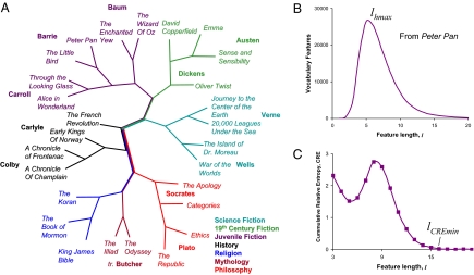
To illustrate FFP text comparison, Fig. 1A shows a neighbor joining tree, which is constructed from FFP distances, each FFP representing the features from one of the e-books. The corpus of books is sampled from several authors and multiple genres/categories (e.g., juvenile fiction, science fiction, etc.). In this example, the FFP method effectively classifies the set of books by subject matter and authorship. Of course, the books are not related to each other by an evolutionary divergence, however, books written by the same author within the same genre tend to share more common features. Similarities in FFP profiles are a result of likeness in vocabulary and diction (i.e., word order) associated with (among many factors) a specific subject matter or topic, reading level and the stylistic preferences of specific authors.

Fig. 1.

Text comparison with FFP. (A) An example of text comparison using the FFP method on English books, each converted into a long character string by removing all punctuation and spaces between words. Books of several different categories/genres are compared. At least 2 books are shown for most authors. High frequency stop features were removed and the feature resolution used is l = 9. (B) Lower limit. Using the children's book Peter Pan as an example, the lower limit of resolution is determined by l_Hmax. (C) Upper limit. Upper limit is determined by l_CREmin.

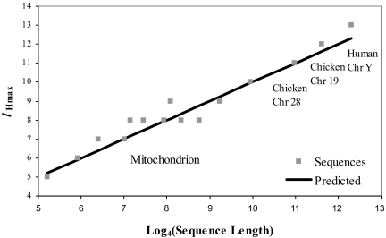
The tree in the above example is constructed specifically with a single feature length (l = 9). However, there are many such trees that can be constructed from different resolutions l. For FFPs derived from a character string, it is possible to determine, a priori, the range of resolutions that are best for representing the string for classification purpose. We have through simulation and observation deduced that this optimal range lies between 2 limits that can be calculated from the character strings themselves. In the children's book Peter Pan, for example, the lower limit (Fig. 1B) is determined by counting the number of vocabulary features (features that occur more than once) in the character string of the book for each l. The peak in this vocabulary feature profile represents the maximum number of different features that can be found in the string, and it occurs at l = l_Hmax. These features are more likely to distinguish this string from other strings. Thus, l_Hmax defines the lower limit of the range of optimal resolution for classification purpose. In general, l_Hmax can be approximated by Eq. 5 for a genome sequence, without empirically determining the peak from the vocabulary feature profile. l_Hmax changes slowly (Fig. 2)—the value increase by 1 when the genome length increases by a factor of 4.

Fig. 2.

Predicted vs. observed l_Hmax. The peak H values, or l_Hmax, for a sample of mitochondrial genomes and chromosomes from human and chicken were observed at different lengths, l.

The value l_CREmin (Fig. 1C), the derivation of which is explained further in Materials and Methods, defines the upper limit of the optimal range for a character string. The upper limit is the length at which the frequencies of all longer features can be accurately estimated using an l-2 Markov estimator. In the case for Peter Pan (a string consisting of ≈172,000 characters), the lower limit is l_Hmax = 6 and the upper limit is l_CREmin = 15. For the books tested here l_Hmax has a value between 5 and 8 and l_CREmin between 15 and 17. The trees constructed using FFPs for l values within the overlapping ranges of l = 9–15 tend to converge upon a single common topology. Also, within this range, statistical resampling tests such as bootstrapping and jackknifing can show that the best supported tree topology largely remains the same for all resolutions within the optimal range. These tests may also be used to assign support to specific clades and groupings. For the rat mitochondrial genome (a string of 16,646 nt), which we use as a test sequence (see below), the limits are l_Hmax = 7 and l_CREmin = 14.

Optimal Resolution Varies with Genome Length.

The optimum range of l for a given genome lies between l_Hmax and l_CREmin. However, because both the upper and lower limit of l are primarily functions of genome length, finding a best l for overlapping ranges can be difficult when comparing genomes with large differences in length. Take for example, the l-mer vocabulary profiles of human chromosome 1 (230 Mbp) and the human mitochondrial genome (16 Kbp), which represent an extreme contrast in both total genome length and l_Hmax. The mitochondrion has l_Hmax = 7, whereas Chr 1 has l_Hmax = 14. This substantial difference in l_Hmax creates a problem finding a common (overlapping) range of l for comparison between genomes of significantly different lengths. However, this is not a serious problem for small genomes, which are approximately the same order of size such as prokaryotes, lower order eukaryotes and viruses.

Robustness of FFP Method with a Test Genome.

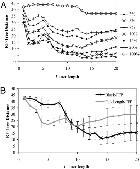
To test the limit of applicability the FFP method, we used a rat mitochondrial genome as a test sequence. The shuffle model (see Materials and Methods) was used to determine the best l for tree reconstruction. Fig. 3A indicates that trees predicted from short l-mers are unreliable and poorly reconstruct the reference tree. The performance of FFP was tested under widely varying base substitution rates. There is a clear dependence between tree distance and substitution rate. For low mutation rates, longer words perform better than features at or near l_Hmax = 7. However, trees constructed with the 10% substitution rate show that there is an optimal l-mer range (l = 10–14), and that longer l-mers (l > 14) less accurately predict the reference tree. In general, the more conserved the sequences, the higher the l that may be safely used.

Fig. 3.

Validation of the optimal feature length range by simulation. (A) Tree reconstruction, using FFP comparison of a divergent sequence population. Ten populations of 25 sequences each with a known lineage (the reference tree) were generated with the shuffle model. The substitution rate was varied in 7 trials. UPGMA tree reconstructions were compared with the reference tree, using the Robinson–Foulds (RF) measure. The significance of the peak near l = 4–5 is not known. (B) Tree reconstruction of different length sequences, full-length-FFP vs. block-FFP comparison. 10 trees of 25 sequences were generated using the excision model. The error bars indicate the standard deviation of the 10 trees. The block-FFP method outperforms the full-length-FFP comparison for l ≥ 11. The block length, m = 16,000 is the length of the smallest genome.

Block-FFP Allows for Comparisons of Widely Different Length Genomes.

As mentioned earlier, the value of l_Hmax increases by 1 for every 4-fold genome length increase (Eq. 10). For comparison of genomes with much greater length differences, we propose to divide (for any pairwise comparison) the larger genome into blocks, which are of equivalent length to the smaller genome. This standardizes the comparison over a single sequence length, and the blocks of the larger genome have similar l-mer vocabulary profiles as the smaller genome, thus the same l_Hmax. A reasonable decision criteria for choosing block comparisons is to evaluate whether there is a relative shift in l_Hmax between compared genomes.

Block-FFP Out-Performs Other Methods for Comparing Different Length Genomes.

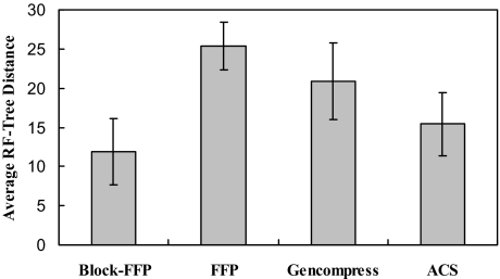
The excision model (see Materials and Methods) population was used to test the effectiveness of block-FFP for standardizing genome comparisons (Fig. 3B). In these tests, genomes differ in length by as much as 8-fold. For l = 1–10 both the blocked and full-length FFP methods are similarly poor in reconstructive ability. In the full-length method the l-mer frequencies for the entire sequences were compared, rather than equal length blocks. However, for l = 11–20 blocked comparisons produce significantly better reference tree reconstructions. Furthermore, the block-FFP method out-performs the ability of the ACS and Gencompress methods (Fig. 4) for comparing genomes with large length differences.

Fig. 4.

Block-FFP vs. other methods: large genome length differences. The methods used are: Block-FFP, blocked comparison, using Eq. 11, and m = 16,000, l = 14; FFP, full-length-FFP comparisons, using Eq. 3 and l = 14; gencompress, normalized complexity distance; ACS, average common substring. Error is the standard deviation.

Example: Intronic Genome Comparison.

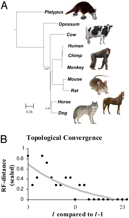
We have tested the applicability of the FFP method for mining phylogenetic information hidden in the intronic regions of whole genomes. All of the known or predicted intron regions were extracted from the deep-coverage (>10×) mammalian genomes and concatenated introns to form an ‘intronic genome.’ Features of lengths 1 to 20 were used to reconstruct trees. As expected from the intronic genome sizes (l_Hmax ≈ 14 for Opossum − the largest) the topologies begin to converge at l = 12 and are fully converged (i.e., the topology of l was equal to l + 1, and all subsequent lengths) at l = 16 (Fig. 6B). Trees from l = 16 to 24 have identical topologies, which confirms the location of the optimal resolution range. The FFP-based topology (Fig. 6A with l = 18) of the “intronic genome” closely reflects the accepted evolutionary history, which has been observed by others, using coding-sequence-based alignment techniques (8). All internal nodes for l > 16 have high jackknife support values (>0.95). This is a particularly interesting result, because it indicates that the intron region contains a similar level of phylogenic signal as do coding exon sequences.

Fig. 6.

FFP comparison of intronic genomes. (A) Concatenated intronic regions of mammals were compared using FFP and RY coding. The tree was constructed with neighbor joining, low complexity, high frequency filtering and l = 18. Nodes indicated have <1.0 jackknife support. Scale indicates Jensen–Shannon divergence length. (B) Topological convergence. A neighbor joining tree was constructed from words of length l = 1–24. The topology of each tree reconstructed from words of length l is compared with trees from l-1. All trees converge to the same topology above l = 16.

Fig. 5.

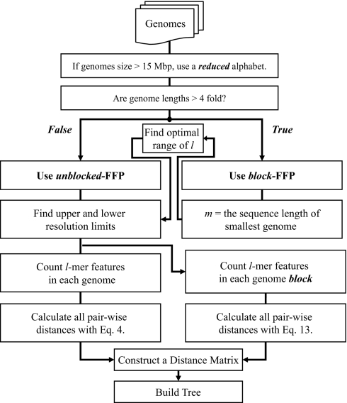
Flow chart of the optimal FFP method.

Discussion

Our method works well over a large range in genome size, if the optimum resolution range is chosen considering several key points that we summarize here.

• The FFP method is particularly useful for comparing whole genomes or genomic regions that have low homology or do not share highly conserved common genes. Large ensembles of introns such as our ‘intronic genomes’, fall into this category, and can be effectively compared using our method.

• The optimum resolution range for a set of genomes can be identified from the overlapping region of the ranges defined by l_Hmax and l_CREmin for each individual genome. From our experience, both with these simulations and with real genomes, only l-mers of lengths greater than the lower boundary of the optimal resolution range should be used for comparison. In the simulated trees, the genome alteration rate also affects the reconstructive ability of different l values. However, even with high alteration rates, the optimum resolution still lies within a predictable range. We found minimal improvement by using especially long l beyond the upper boundary of the optimal range. More importantly, the inclusion of much longer l, beyond the upper bound for more divergent genomes can significantly worsen the predicted tree topology when the compared FFPs of whole genomes are highly divergent, as are the cases with viral or mammalian genomes. This is probably because the features with l > l_Hmax are mostly populated by those that occur only once among all genomes compared.

• The values of l_Hmax and l_CREmin for a given genome are largely dependant on the genome length. Thus, the significance of length differences among compared genomes should be carefully considered. Length differences only become significant when >4-fold when nucleotide sequences are considered, or 20-fold in the case of protein sequences. In these cases block-FFP should be considered. Length differences of lesser magnitude are unlikely to necessitate block-FFP.

This method should prove useful for group assignment of new genomes of low homology, for comparing metagenomes, incomplete and fragmentary genomes, and for mining nongenic regions of whole genomes.

Materials and Methods

The FFP alignment-free method consists of 3 major steps: (i) testing whether the lengths of the shortest and the longest genomes differ by more than 4-fold, (ii) determining the optimal resolution range for genomes compared and (iii) comparing FFPs, using the Jensen–Shannon (JS) Divergence. For whole-genome sequences, our method was validated by evaluating its ability to regenerate the topology of a reference tree. For comparing phylogenies, we compared UPGMA (9) trees produced from JS divergence information to the reference tree, using the phylip package (10). Later examples use the Neighbor Joining method (11). The advantage of using this simulated data is that the topology of the reference tree is known with absolute certainty. This method of validation is similar to a study by Hohl et al. (12). To compare FFP tree topologies to the reference tree, we used the symmetric tree distance or Robinson–Foulds distance (13), as implemented in the treedist program of phylip. This distance is equal to the minimum number of operations, consisting of merging or splitting nodes, necessary to transform one tree into the other. For our purposes the results based on RF distance were almost identical to those based on another distance metric, the maximum agreement subtree (14). The details of the key processes in the FFP method are described below:

Feature Frequency Profiles (FFP).

To count the frequencies of each feature in the genome, a sliding window of length l is run through the sequence from position 1 to n − l + 1. Large genomes, which consist of multiple chromosomes, are represented by a collection of assembled chromosomes and others are just a collection of unassembled contigs. When counting, l-mers continue over the whole genome, but the sliding window is not allowed to span over sequencing gaps. The counts are tabulated in the vector C_l for all possible features of length l,

where K, the number of all possible features, is 4^l and 4 is the alphabet size. The raw frequency counts are normalized to form a probability distribution vector or FFP,

giving the relative abundance of each l-mer. This normalization removes small genome length differences as a factor in the comparison, however, for larger differences, see Block-FFP.

Genome Comparison with Jensen–Shannon Divergence.

The distance between 2 probability vectors P_l and Q_l is calculated using the Jensen–Shannon (JS) Divergence,

where M_i = (P_i + Q_i)/2 and KL is the Kullback-Leibler divergence,

The JS divergence is a convenient divergence measure for our purpose because it is symmetric and bounded between 0 and 1. Note, that the JS divergence is not strictly a metric distance as it does not always satisfy triangle inequality. See Lin (15) for a further description.

Lower Limit of Resolution: Vocabulary Features and l_Hmax.

Reliable resolutions always fall into a particular range of an l-mer vocabulary feature profile, H. Vocabulary features are those features occurring more than once in a genome. The profile, H, is constructed by counting the number of vocabulary features for each l. The location of the peak in the distribution, i.e., the l with the largest vocabulary, is related to the sequence length, n. The l with maximum H, l_Hmax is empirically determined but may be closely approximated by,

where 4 is the alphabet size. Fig. 2 shows a fit of eq. 5 to genome sequence data. We have observed empirically and through our validation tests that reliable tree topologies are typically obtained with l-mer resolutions where l>l_Hmax whereas lengths below l_Hmax yield unreliable trees.

Upper Limit of Resolution: Cumulative Relative Entropy (CRE).

The upper limit of resolution can be empirically determined by a criterion that the tree topology for feature length l is equal to that of l + 1, i.e., tree topologies converge. This convergence criterion can be used to find the upper limit for large genomes (such as the mammalian intron genomes) or in cases where not computationally prohibitive, the upper limit can also be derived by using the concept of cumulative relative entropy. Briefly, we can estimate the FFP for length, l, from the FFPs of l-1 and l-2, using an l-2 Markov chain model. The expected frequency, f̂_l, of an l-mer given the prior knowledge of the FFP probability distribution of l-1 and l-2 is,

where fa₁a₂ … a_l is the frequency of a l-mer formed from the letters a₁a₂ … a_l. An expected FFP, F̂_l, can be found from F_l-1 and F_l-2. Further, F̂_l and F_l-1 can be used to find F̂_l+1, and thus all F̂_l+k up to infinite k can be found by iteratively applying Eq. 6 to find the next longest expected FFP.

To measure how close the expected frequency is to the observed frequency for the entire probability distribution, we compute the relative entropy (eq 4):

We define cumulative relative entropy (CRE) at l as the sum of relative entropy from l to infinity (but in practice one can stop when KL ≈ 0):

The CRE represents the accuracy of predicting FFPs for all lengths greater than or equal to l, given the prior distributions F_l-1 and F_l-2. If a given sequence has zero CRE at feature length l, then the FFPs F_l-1 and F_l-2 have all of the information necessary to form longer features. When CRE approaches zero, this value of l delineates the upper limit for use in genome comparison (see Fig. 1C). We designate this point as l_CREmin.

Constructing the Simulated Phylogenic Ancestry.

The tests presented here were specifically designed to test the limit of applicability for the FFP method. Thus, high rates of substitution and rearrangement are used to push the divergence to the point where sequence alignment is no longer useful for constructing phylogenies. The models below are not meant to realistically describe the mutational processes occurring across short time spans. The models are based on an accelerated and exaggerated mode of genomic rearrangement so that significant rearrangement and divergence will occur within 20 generations of computer simulation. For computational expediency a short mitochondrial sequence is chosen as a root ancestor test sequence. Two child genomes are copied from this initial parent with an underlying genome alteration model.

We used 2 models: (i) shuffle and (ii) excision. The shuffle model involves 2 components: (i) rearrangement, a random excision and reinsertion of a sequence fragment that occurs once per duplication and (ii) mutation, a random base substitution that occurs at a fixed percentage rate. The Rattus norvegicus mitochondrion was used as the ancestor sequence and the excised fragment size can be up to 0.1n in length (where n is the length of the genome sequence). After a set of sequences is evolved, the result is a set of equal length sequences with a known lineage.

Likewise, the excision model consists of 2 elements: (i) a random excision without replacement, of a sequence fragment that occurs once per duplication and (ii) mutation, random base substitution that occurs at 10% of base positions. The root ancestor in this case is generated by randomly concatenating 25 mitochondrial sequences. The excision is the same length as above. In contrast to the shuffle model, we obtain a set of divergent sequences with varying lengths. We selected sets of sequences with as much as an 8-fold difference in length from the smallest to largest descendant genome. These sets were used to validate the effectiveness of block-FFP comparisons under extreme conditions.

A synthetic lineage with a known tree is created using one of the above genome alteration models. However, for simplicity, we did not include any selection process in effect during the simulation. Each child is set to have a 1 in 4 chance of going extinct and the parent generation at each level dies. Children are produced up to the 20th generation. The ancestral history of the children at the leaf nodes forms the reference tree topology. These reference trees were used to validate our method.

Filtered Feature Sets and the Reduced Purine-Pyrimidine Alphabet.

The use of all possible l-mers for especially long genomes or especially long l has computer memory allocation limitations, so feature filtering may be necessary. One effective form of l-mer filtering is to assume that some words are degenerate because sequence evolution is indeed tolerant of many kinds of sequence substitutions. For nucleotide sequences, the bases A and G (both purine bases), and C and T (both pyrimidines) can form 2 equivalent classes R and Y. This reduced alphabet is especially useful for comparing large genomes, because it substantially reduces memory allocation requirements. Also, the R-Y alphabet has been shown to improve phylogenies by removing the distorting effects of species specific bias in base composition and bias in the third codon position (8, 16). A further reduction can be accomplished by establishing equivalency between the reverse complement and its forward sequence. In validation tests, no filtering was applied and the full 4 letter alphabet was used.

Removal of High Frequency and Low Complexity Features.

The genomes of higher order Eukaryotes contain a large fraction of sequence that is repetitive or of low complexity, most often in nongenic or intergenic regions. The complexity of a feature, K_f, is determined by comparing its size in bytes, before and after lossless compression.

The compression is implemented using the gzip utility (gzip −9). For an example of complexity values, the most and least complex features for l = 18 have K_f of 16 and 5 respectively. Gencompress (21), a method developed for compression of DNA sequences, was also tried, but gave approximately equal complexities for all features of a given length because it is optimized to compress whole-genome sequences, not features. The complexity of l-mers for a given l is normally distributed, and one can choose only the most complex features, which are generally of low frequency.

Also, high frequency features should be disregarded because they are usually not sensitive to distinguishing different genomes, and these features tend to dominate the Jensen–Shannon distance score. No complexity or high frequency filtering was applied to the validation tests of the short sequences.

Block-FFP/Full-Length-FFP Distance Comparison.

Full-length-FFP comparisons are implemented using pairwise JS distances (Eq. 3). This method is best used on approximately equal length sequences (<4-fold different). Genomes with large differences in length can be compared effectively, using the block-FFP method. Block comparisons are an absolute necessity when comparing genomes with large length differences. A reasonable decision criterion for choosing block-FFP is to evaluate whether there is a relative shift in l_Hmax between compared genomes. According to Eq. 5 this is a length difference of,

where the genome length, n_j, is greater than n_i and 4 is the base alphabet size. Note, for comparison of large chromosomes we have used a simplified 2-letter alphabet. The block method is similar to that described by Wu et al. (17). When sequences a and b are compared, each sequence is divided into m length blocks. For a set of genomes the block size should be the size of the smallest genome. If a genome is not evenly divisible by m then blocks overlap by n modulus m bases. Sequence a and b have A and B numbers of blocks, respectively. The block distance may be computed as,

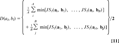where a_i and b_j represent the FFPs derived from the blocks of sequences a and b, and min is the minimum distance, among the set of distances. In this case JS_l is the distance between each block-to-block comparison. The block distance calculates the average JS distance of the best matches between all pairs of sequence blocks. Blocked FFPs are used when comparing genomes of diverse size.

Other Methods: Average Common Substring and Compression Based Distances.

We compared the FFP and block-FFP methods to 2 other alignment free methods. The average common substring (ACS) distances were calculated as described by Ulitsky et al. (18). ACS finds the average length of the longest substrings starting at every sequence position that are shared between 2 sequences. A normalized compression distance can be formed from the Kolmogorov complexity of a, K_a, which is defined as the length of the smallest program that will produce the output a (19, 20). K_a is approximated by finding the size of a after lossless compression, k_a. A sequence distance can be formed using the approximated k,

where k_a and k_b are the compressed sizes of sequence a and b, and k_ab and k_ba are the compressed sizes of the concatenated sequences. The software, Gencompress, is used as the lossless compression algorithm (21).

Text Comparison.

The books used in the text example were obtained from the Project Gutenberg database (www.gutenberg.org). E-text numbers used: 11, 12, 16, 17, 36, 55, 150, 158, 161, 164, 518, 730, 766, 1301, 1376, 1656, 1728, 1932, 2199, 2412, 2800, 4213, 5146, 8438, 10900, and 18857. Each text was preprocessed by removing file headers, footers, title, chapter, author information and several high frequency stop words: “and,” “the,” “a,” and “an.” All nonalphabetic characters and spaces were deleted. Vocabulary feature and CRE profiles were constructed, and the lower and upper limits were respectively, l_Hmax = 6 and l_CREmin = 15. Fig. 1 was constructed with Eq. 3 and l = 9.

Mammalian Intronic Genome Comparison.

To investigate the evolutionary information contained within intron sequences, all annotated and predicted introns were extracted from the complete reference genomes of Human (Homo sapiens), Chimpanzee (Pan troglodytes), Rhesus Monkey (Macaca mulatta), Mouse (Mus musculus), Rat (Rattus norvegicus), Dog (Canis lupus familiaris), Horse (Equus caballus), Cow (Bos taurus), Opossum (Monodelphis domesticus), and Platypus (Ornithorhynchus anatinus). These genomes have the deepest sequencing coverage (>10×). Intron sequences were extracted from the genbank assembly records found at National Center for Biotechnology Information (ftp://ftp.ncbi.nlm.nih.gov/genomes), using the base pair positions specified by each genbank CDS field. All introns from a species were concatenated together in 1 intron genome file with an x character separating each intron. The separator prevents extracted features from spanning 2 introns. It is worth noting that the GenBank annotations are known to be incomplete, so our genome partitions will necessarily misallocate a number of un-annotated or poorly predicted introns. The relative sizes of all of the intronic genomes are approximately similar (within 4-fold), ranging from 391 Mbps in platypus to 947 Mbps in Opossum. The reduced RY coding scheme was used in this case. Low complexity filtering was applied to the mammalian intronic genomes by removing all features less complex than μ-σ in complexity (where μ and σ are the mean and standard deviation of the feature complexities in the feature set). High frequency features were removed by only choosing those features with feature counts less than μ + σ (where μ and σ represent the mean and deviation of feature counts for all genomes in the set). The time limiting step in the FFP method is feature counting. The longest intronic genome, the Opposum, took ≈5 min to count and assemble the complete FFP profile (l = 18), using a 2.1 GHz CPU. Neighbor joining trees were constructed for all lengths l (Fig. 6A, l = 18 shown) and tree topologies were compared with the RF distance measure (Fig. 6B). To establish support for the topology at each length l we used a jackknife form of resampling, where we sampled 10% of the total features after complexity filtering (without replacement) for a given l. Support values in Fig. 6A were obtained from 10,000 replicates.

References

- 1.Wildman DE, et al. Genomics, biogeography, and the diversification of placental mammals. Proc Natl Acad Sci USA. 2007;104:14395–14400. doi: 10.1073/pnas.0704342104. [DOI] [PMC free article] [PubMed] [Google Scholar]
- 2.Huynen MA, Bork P. Measuring genome evolution. Proc Natl Acad Sci USA. 1998;95:5849–5856. doi: 10.1073/pnas.95.11.5849. [DOI] [PMC free article] [PubMed] [Google Scholar]
- 3.Venter JC, et al. The sequence of the human genome. Science. 2001;291:1305–1350. [Google Scholar]
- 4.Berney E, et al. Identification and analysis of functional elements in 1% of the human genome by the ENCODE pilot project. Nature. 2007;447:799–816. doi: 10.1038/nature05874. [DOI] [PMC free article] [PubMed] [Google Scholar]
- 5.Deerwester S, et al. Indexing by latent semantic analysis. J Am Soc Inform Sci. 1988;41:391–407. [Google Scholar]
- 6.Blaisdell BE. A measure of the similarity of sets of sequences not requiring sequence alignment. Proc Natl Acad Sci USA. 1986;83:5155–5159. doi: 10.1073/pnas.83.14.5155. [DOI] [PMC free article] [PubMed] [Google Scholar]
- 7.Vinga S, Almeida J. Alignment-free sequence comparison: A review. Bioinformatics. 2003;19:513–523. doi: 10.1093/bioinformatics/btg005. [DOI] [PubMed] [Google Scholar]
- 8.Prasad AB, Allard MW. Confirming the phylogeny of mammals by the use of large comparative sequence data sets. Mol Biol Evol. 2008;25:1795–1808. doi: 10.1093/molbev/msn104. [DOI] [PMC free article] [PubMed] [Google Scholar]
- 9.Sneath PHA, Sokal RR. Numerical Taxonomy. San Francisco: W.H. Freeman; 1973. pp. 230–234. [Google Scholar]
- 10.Felsenstein J. PHYLIP—Phylogeny Inference Package (Version 3.2) Cladistics. 1989;5:164–166. [Google Scholar]
- 11.Saitou N, Nei M. The neighbor-joining method: A new method for reconstructing phylogenetic trees. Mol Biol Evol. 1987;4:406–425. doi: 10.1093/oxfordjournals.molbev.a040454. [DOI] [PubMed] [Google Scholar]
- 12.Hohl M, et al. Pattern-based phylogenetic distance estimation and tree reconstruction. Evol Bioinf Online. 2004;2:357–373. [PMC free article] [PubMed] [Google Scholar]
- 13.Robinson DR, Foulds LR. Comparison of phylogenetic trees. Math Biosci. 1981;53:131–147. [Google Scholar]
- 14.Steel M, Warnow T. Kaikoura tree theorems: Computing the maximum agreement subtree. Inform Process Lett. 1993;48:77–82. [Google Scholar]
- 15.Lin J. Divergence measures based on the Shannon entropy. IEEE T Inform Theory. 1991;37:145–151. [Google Scholar]
- 16.Phillips MJ, et al. Genome-scale phylogeny and the detection of systematic biases. Mol Biol Evol. 2004;21:1455–1458. doi: 10.1093/molbev/msh137. [DOI] [PubMed] [Google Scholar]
- 17.Wu TJ, et al. Optimal word sizes for dissimilarity measures and estimation of the degree of dissimilarity between DNA sequences. Bioinformatics. 2005;21:4125–4132. doi: 10.1093/bioinformatics/bti658. [DOI] [PubMed] [Google Scholar]
- 18.Ulitsky I, et al. The average common substring approach to phylogenomic reconstruction. J Comp Biol. 2006;13:336–350. doi: 10.1089/cmb.2006.13.336. [DOI] [PubMed] [Google Scholar]
- 19.Li M, et al. An information-based sequence distance and its application to whole mitochondrial genome phylogeny. Bioinformatics. 2000;17:149–154. doi: 10.1093/bioinformatics/17.2.149. [DOI] [PubMed] [Google Scholar]
- 20.Mantaci S, et al. Distance measures for biological sequences: Some recent approaches. Int J Approx Reason. 2008;47:109–124. [Google Scholar]
- 21.Chen X, et al. A compression algorithm for DNA sequences based on approximate matching. Proceedings of the Fourth Annual International Conference on Computational Molecular Biology (RECOMB); Tokyo, Japan. New York: Association for Computing Machinery; 2000. p. 107. [Google Scholar]