

Abstract
Quantitative magnetization transfer imaging (qMTI) methods are able to estimate fundamental sample parameters, such as the relative size of the solid-like macromolecular proton pool and the spin exchange rate between this pool and the directly measured free water protons. One such method is selective inversion recovery (SIR), in which the free water protons are selectively inverted and the signal is fit to a biexponential function of the inversion time (TI). SIR uses only low-power pulses and requires no separate RF (B1) or static field (B0) field maps, and the analysis is largely independent of the macromolecular pool lineshape. These are all advantages over steady-state off-resonance saturation qMTI methods. However, up to now, SIR has been implemented only with repetition times TR ≫ T1. This paper describes a modification of SIR with smaller TR values and a greater signal-to-noise ratio (SNR) efficiency.
Keywords: MT, qMT, qMTI, quantitative myelin
qMTI estimates inherent magnetization transfer (MT) sample properties. Unlike the more widely implemented qualitative technique based on MT ratios (MTRs), which acquires simple ratio images with and without off-resonant RF saturation pulses, qMTI is a quantitative technique that estimates several MT parameters independently of relaxation rates and the details of the pulse sequence timings and powers. As such, qMTI offers the possibility of achieving greater specificity and more accurate comparisons among scanners and individuals. Such benefits have recently generated considerable interest in various applications (1–6), such as the quantification of myelin.
The development of qMTI acquisition techniques is still an active area, with methods falling into one of two general categories: steady-state and transient. Steady-state methods (5–9) are pulsed variations of Henkelman et al.’s (10) off-resonance saturation technique, while the transient methods (11–15) are pulsed variations of Wolff and Balaban’s (16) and Eng et al.’s (17) approach to steady state in the presence of RF irradiation, or Edzes and Samulski’s (18,19) approach to steady state in the absence of RF irradiation. The present method falls into the latter category and is most closely related to the method of Gochberg and Gore (12), except that it uses arbitrary TRs.
THEORY
The selective-inversion-recovery fast-spin-echo (SIR-FSE) imaging pulse sequence is diagrammed in Fig. 1a. The essential insight is that at the end of each repetition, both the macromolecular and free water pools have zero z-magnetization. The free water protons have zero z-magnetization due to the 90° pulse (which rotates the z-magnetization into the transverse plane), followed by the series of closely spaced refocusing 180° pulses (which prevent any effective T1 recovery by inverting the z-magnetization before there is substantial regrowth). The macromolecular protons are not affected by the low-power 90° pulse. However, they are pulled toward the nulled free water z-magnetization by the MT effect on a time scale of 1/ R1+ ∼40 ms (in the brain). If the z-magnetization of the free water protons is held at zero for a time ≫ 40 ms, the macromolecular protons will be effectively nulled. As shown below, under such conditions the analysis is identical to the long-TR case except that the calculated value of the macromolecular z-magnetization after the initial 180° pulse is multiplied by a factor of 1 — exp(-R1- td), where R1– is the slow recovery rate (often equated with the observed R1 value) and td is defined in Fig. 1a.
FIG. 1.

a: SIR with an FSE readout. Each acquisition is made through a different line of k-space. td is the delay from the last 180° pulse until the next repetition. Multiple images are acquired and fit to a biexponential function of ti. b: The simulated evolution of the normalized z-magnetization of the free (dashed) and macromolecular (solid) proton pools. Note the roughly exponential decay of Mm(t)/Mm∞ during the FSE evolution with a time constant of 1/kmf. After the RF pulse train, both proton pools recover together with the longer time constant 1/R1–. The parameter values used for the simulation were R1f = 1 Hz, R2f = 25 Hz, R1m = 1 Hz, R2m = 100 kHz, kfm = 3 Hz, kmf = 30 Hz, pulse width = 1.5 ms, ti= 50 ms, echo spacing = 10 ms, and eight echoes. The blips of Mf(t)/Mf∞ during the FSE evolution are due to the rotation during the RF pulses and are not important for our results.
This result can be derived by considering the recovery of the magnetization when there are no RF pulses (12,18–20):
| [1] |
where
| [2] |
| [3] |
where R1- and R1+ are the slow and fast recovery rates, respectively, with corresponding amplitudes bf– and bf+. The subscripts f and m refer to the free solvent and macromolecular (immobile) proton pools, respectively. Mf(t) and Mm(t) are the longitudinal magnetizations at time t, whose equilibrium values are Mf∞ and Mm∞. R1f and R1m are the longitudinal relaxation rates of the mobile and macromolecular protons when there is no MT between them. kfm is the MT rate from the free to the macromolecular pool, kmf is the rate in the reverse direction, and kfm/kmf is equal to the pool size ratio (pm/pf).
The typical analysis assumes a kmf that is much larger than any other rate, giving
| [4] |
and
| [5] |
This assumption allows one to determine kmf and pm/pf by fitting for R1+, , , and Mf(0)/Mf∞ and numerically simulating the saturation effect of the RF inversion pulse to determine Mm(0)/M∞ (assuming a rough estimate of T2m, a pulse duration that is much shorter than 1/R1m), and a TR ≫ ). That is,
| [6] |
where Sm is the simulated saturation effect of the RF pulse (0.83 ± 0.07 for a 1-ms hard inversion pulse on a solid pool with a Gaussian lineshape and a T2 between 10 μs and 20 μs, calculated as in Ref. 13). This determination of Sm is the only time when lineshape assumptions are relevant, and in contrast to the case of off-resonant saturation, such assumptions only have a small effect on the determined MT parameter values.
In the current work, no restriction on the TR is required. Instead, we assume zero z-magnetization after the last 180° pulse in the FSE train. The biexponential recovery during the time td is then (to first order in 1/kmf):
| [7] |
giving
| [8] |
Likewise,
| [9] |
While Mf(0)/Mf∞ is still directly measured (thereby making the use of Eq. [9] unnecessary), for the short-TR case, Eq. [8] is used instead of Eq. [6] to estimate the pool size ratio via Eq. [5]. That is, in summary, the measured signal (as a function of the inversion time (TI), t) is fit to Eq. [1] to determine R1+, R1-, and Mf∞. Numerical simulations give Sm. The rate kmf is calculated using Eq. [4], and the pool size ratio pm/pf is calculated using Eqs. [1], [5], and [8]:
| [10] |
If we ignore the uncertainties in the numerically determined Sm, propagation of errors gives a pm/pf signal-to-noise ratio (SNR) that is proportional to (1 — exp(-R1– td)). Therefore the SNR in a given measurement time is
| [11] |
Figure 2 plots Eq. [11] as a function of td. Note that lowering td from 10 s (as required when near-complete recovery is demanded) to ∼2.5 s not only increases the speed of the measurement but also increases the SNR efficiency by roughly 50%.
FIG. 2.
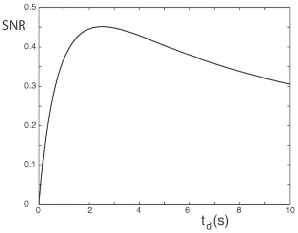
SNR (in arbitrary units) for an SIR-FSE imaging experiment in a given measurement time vs. td according to Eq. [10]. The parameters are R1– = 0.65 Hz, ti,average = 565 ms, and FSE pulse train = 100 ms. The maximum SNR efficiency is at td = 2.5 s.
Note that this analysis requires that the predelay td is held constant as the inversion time ti is varied. If instead the TR is held constant, as in the modified fast IR sequence (21), the analysis is complicated by a third component with a recovery rate R1+ — R1-.
MATERIALS AND METHODS
To confirm that the macromolecular z-magnetization is zero at the end of the FSE pulse train, we simulated the evolution using six coupled differential equations (10). We also implemented SIR-FSE imaging at 9.4T with an FOV of 45 × 45 × 3 mm and a resolution of 96 × 96 processed to 128 × 128, 16 echos, echo spacing = 5ms, td = 3.5 s, one dummy scan, and ti = 25 values (21 points logarithmically spaced between 3.5 ms and 150 ms, and 300 ms, 1 s, 2 s, and 10 s). The total acquisition time was 21 min.We applied this method to 10% cross-linked bovine serum albumin (BSA) to test the validity of the method, and to in vivo ferret brain to demonstrate the sequence and analysis in a more typical system of interest. The ferret was anesthetized using an IM injection of Telasol (22 mg/kg) and maintained on isofluorane/oxygen gas mixture at 1.5% with continuous monitoring and maintenance of respiratory rate and CO2. The Vanderbilt Institutional Animal Care and Use Committee approved all of the animal procedures. Least-square fitting of the data was performed using Matlab’s built-in Nelder-Mead simplex method.
RESULTS
Numerical Simulations
The central premise of our analysis of the short-TR SIR-FSE qMTI method is that the z-magnetization of both proton pools is approximately zero at the end of the FSE readout period. Figure 1b plots the results of simulations and demonstrates that the z-magnetization of the free pool is nulled during the FSE readout, and the z-magnetization of the macromolecular proton pool decays roughly exponentially to zero at a rate of kmf. Figure 3 plots the zmagnetization remaining after the FSE readout as a function of the MT rate kmf, and demonstrates that the zmagnetization of both pools are effectively nulled as long as kmf is not too small.
FIG. 3.
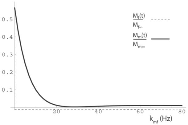
The simulated normalized z-magnetization of the free (dashed) and macromolecular (solid) proton pools at the end of the FSE pulse train as a function of the fast MT rate kmf(at t = 0.127 s in Fig. 1). The other parameters are the same as in Fig. 1, but with kfm = 0.1 kmf. Note that the z-magnetization magnitude of both pools is less than 1.5% of their equilibrium values for kmf > 19 Hz.
Table 1 gives the results of fitting simulated data using reasonable values for the MT and relaxation parameters of white matter, gray matter, and muscle. The key result is that any nonzero z-magnetization after the FSE readout has a negligible effect, but taking the approximations inherent in Eqs. [4] and [10] causes systematic errors of 8–19% in kmf and 5–12% in pm/pf.
Table 1.
| kmf WM | pm/pf WM | kmf GM | pm/pf GM | kmf Mus. | pm/pf Mus. | |
|---|---|---|---|---|---|---|
| Input parameters | 15 | 0.155 | 28 | 0.059 | 46 | 0.108 |
| Parameters determined using data created using Bloch equations |
17.85 | 0.1364 | 30.15 | 0.0556 | 51.47 | 0.0972 |
| Parameters determined using data created by nulling z- magnetization |
17.85 | 0.1367 | 30.15 | 0.0558 | 51.47 | 0.0974 |
The data is created by either integrating the coupled Bloch equations (the more realistic method) or by setting the z-magnetization of both pools to zero at the end of the FSE pulse train. Other parameters are td = 2s, R1m = 0.5 Hz, R2m = 100000 Hz, andR1f = 0.66 Hz, R2f = 25 Hz for white matter (WM), R1f = 0.52 Hz, R2f = 22 Hz for gray matter (GM), and R1f = 0.49 Hz, R2f = 33 Hz for muscle (M). Sequence parameters are as in Fig. 1. Note that deviations from zero z-magnetization after the FSE pulse train have only a minor effect on pm/pf and no effect on kmf. The difference between the fitted parameters and the input parameters is due nearly entirely to taking only a first order approximation in 1/kmf in Eqs. [4] and [10].
Measurements
Figure 4 plots the results of applying reduced-TR SIR-FSE imaging to 10% cross-linked BSA. Note the key result that the pool size ratio calculated using Eq. [10] is independent of the delay between repetitions (though the uncertainty is not, as expected).
FIG. 4.
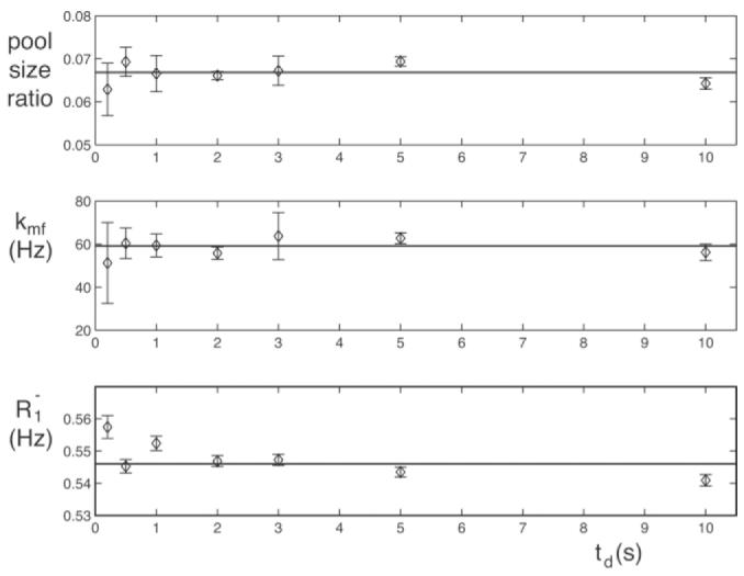
Sample parameters of 10% cross-linked BSA as determined by SIR-FSE imaging vs. td. The pool size ratio is calculated from Eq. [10], kmf comes from Eq. [4], and R1– is the fitted slow recovery rate. Plotted values are the mean ± SD of 25 central pixels. The solid line is the weighted mean at all td values. Note that the results are independent of td, except perhaps for a slight trend in R1–, which is likely a result of sample heating during the measurement.
Figure 5 illustrates in vivo SIR-FSE imaging in a ferret in vivo. Table 2 gives the results for the white matter, gray matter, and muscle regions illustrated in Fig. 6.
FIG. 5.

Fast repetition SIR-FSE qMTI of a ferret. kmf is the MT rate from the macromolecular pool to the free water pool.
Table 2.
| White matter | Cortical gray matter |
Subcortical gray matter |
Muscle | |
|---|---|---|---|---|
| kmf (Hz) | 14.9 ± 1.4 | 30 ± 3 | 25 ± 3 | 46 ± 3 |
| pm/pf | 0.155 ± 0.006 | 0.057 ± 0.004 | 0.063 ± 0.003 | 0.108 ± 0.003 |
Parameters are the mean ± standard deviation (SD) of the values of the selected pixels.
FIG. 6.

Region map of white matter (red), gray matter (green and blue), and muscle (purple). The underlying image is a SIR with ti = 300 ms. Table 2 lists the corresponding MT parameters.
DISCUSSION
SIR-FSE imaging with reduced TR provides an efficient means of performing qMTI and compares favorably with pulsed saturation techniques (such as those of Sled et al. (3)). Specifically, pulsed saturation qMTI requires nontrivial pulse programming, complicated data fitting, assumptions concerning the macromolecular lineshape, and separate T1,RF (B1), and static field (B0) maps. SIR-FSE imaging is simpler to program, involves a simpler data analysis, makes only small assumptions concerning the lineshape (though it does make stronger, though reasonable, assumptions concerning the macromolecular transverse relaxation rate and kmf), and requires only low-power RF pulses. This use of only low-power RF pulses may be especially important. Since pulsed saturation manipulates the wide-bandwidth macromolecular pool, it will always be constrained by the amplifier power and SAR limits of clinical MRI systems. By directly manipulating only the free water pool, SIR avoids these power issues and therefore may ultimately prove to be better suited for performing clinical qMTI. However, a significant shortcoming of SIR-FSE is that the current analysis does not allow for multislice imaging (where the refocusing pulses will cause MT effects on other slices) and the systematic parameter biases illustrated in Table 1. Also, pulsed saturation has two strengths: it has been extensively tested in in vivo studies, and it can be used to quantify the macromolecular transverse relaxation rate. The acquisition parameters of the two sequences have not been optimized, and no careful comparisons of the two methods in terms of achievable accuracy and precision have been performed.
By comparing our results in Table 2 with those acquired via pulsed saturation by Sled et al. (3,4) (and ignoring the small number of data points, the differences in field strength, and differences between human and ferret brains), one can see a rough agreement for the pool size ratios but a significant difference in the MT rate kmf(which corresponds to kf/F in the pulsed saturation results). In white matter in particular, Sled et al. obtained values roughly 100% larger than ours. This result is not surprising, given the reported difficulty of using pulsed saturation to determine kf (9). It also suggests that pulsed saturation and SIR may provide complementary information for determining MT parameters. In any case, a full determination of the relative strengths of these two approaches is beyond the scope of the current work.
ACKNOWLEDGMENTS
We thank Adrienne Dula and Mark Does for assistance in the data acquisition.
Grant sponsor: National Institutes of Health; EB001452; EB000214; EB001744; Grant sponsor: NCRR; Grant number: 1S10 RR17799.
REFERENCES
- 1.Levesque I, Sled JG, Narayanan S, Santos AC, Brass SD, Francis SJ, Arnold DL, Pike GB. The role of edema and demyelination in chronic T1 black holes: a quantitative magnetization transfer study. J Magn Reson Imaging. 2005;21:103–110. doi: 10.1002/jmri.20231. [DOI] [PubMed] [Google Scholar]
- 2.Narayanan S, Francis SJ, Sled JG, Santos AC, Antel S, Levesque I, Brass S, Lapierre Y, Sappey-Marinier D, Pike GB, Arnold DL. Axonal injury in the cerebral normal-appearing white matter of patients with multiple sclerosis is related to concurrent demyelination in lesions but not to concurrent demyelination in normal-appearing white matter. Neuroimage. 2006;29:637–642. doi: 10.1016/j.neuroimage.2005.07.017. [DOI] [PubMed] [Google Scholar]
- 3.Sled JG, Levesque I, Santos AC, Francis SJ, Narayanan S, Brass SD, Arnold DL, Pike GB. Regional variations in normal brain shown by quantitative magnetization transfer imaging. Magn Reson Med. 2004;51:299–303. doi: 10.1002/mrm.10701. [DOI] [PubMed] [Google Scholar]
- 4.Sled JG, Pike GB. Quantitative imaging of magnetization transfer exchange and relaxation properties in vivo using MRI. Magn Reson Med. 2001;46:923–931. doi: 10.1002/mrm.1278. [DOI] [PubMed] [Google Scholar]
- 5.Tozer D, Ramani A, Barker GJ, Davies GR, Miller DH, Tofts PS. Quantitative magnetization transfer mapping of bound protons in multiple sclerosis. Magn Reson Med. 2003;50:83–91. doi: 10.1002/mrm.10514. [DOI] [PubMed] [Google Scholar]
- 6.Yarnykh VL. Pulsed Z-spectroscopic imaging of cross-relaxation parameters in tissues for human MRI: theory and clinical applications. Magn Reson Med. 2002;47:929–939. doi: 10.1002/mrm.10120. [DOI] [PubMed] [Google Scholar]
- 7.Lee RR, Dagher AP. Low power method for estimating the magnetization transfer bound-pool macromolecular fraction. J Magn Reson Imaging. 1997;7:913–917. doi: 10.1002/jmri.1880070521. [DOI] [PubMed] [Google Scholar]
- 8.Ramani A, Dalton C, Miller DH, Tofts PS, Barker GJ. Precise estimate of fundamental in-vivo MT parameters in human brain in clinically feasible times. Magn Reson Imaging. 2002;20:721–731. doi: 10.1016/s0730-725x(02)00598-2. [DOI] [PubMed] [Google Scholar]
- 9.Sled JG, Pike GB. Quantitative interpretation of magnetization transfer in spoiled gradient echo MRI sequences. J Magn Reson. 2000;145:24–36. doi: 10.1006/jmre.2000.2059. [DOI] [PubMed] [Google Scholar]
- 10.Henkelman RM, Huang X, Xiang Q, Stanisz GJ, Swanson SD, Bronskill MJ. Quantitative interpretation of magnetization transfer. Magn Reson Med. 1993;29:759–766. doi: 10.1002/mrm.1910290607. [DOI] [PubMed] [Google Scholar]
- 11.Chai J-W, Chen C, Chen JH, Lee S-K, Yeung HN. Estimation of in vivo proton intrinsic and cross-relaxation rates in human brain. Magn Reson Med. 1996;36:147–152. doi: 10.1002/mrm.1910360123. [DOI] [PubMed] [Google Scholar]
- 12.Gochberg DF, Gore JC. Quantitative imaging of magnetization transfer using an inversion recovery sequence. Magn Reson Med. 2003;49:501–505. doi: 10.1002/mrm.10386. [DOI] [PubMed] [Google Scholar]
- 13.Gochberg DF, Kennan RP, Robson MD, Gore JC. Quantitative imaging of magnetization transfer using multiple selective pulses. Magn Reson Med. 1999;41:1065–1072. doi: 10.1002/(sici)1522-2594(199905)41:5<1065::aid-mrm27>3.0.co;2-9. [DOI] [PubMed] [Google Scholar]
- 14.Ropele S, Seifert T, Enzinger C, Fazekas F. Method for quantitative imaging of the macromolecular 1H fraction in tissues. Magn Reson Med. 2003;49:864–871. doi: 10.1002/mrm.10427. [DOI] [PubMed] [Google Scholar]
- 15.Tyler DJ, Gowland PA. Rapid quantitation of magnetization transfer using pulsed off-resonance irradiation and echo planar imaging. Magn Reson Med. 2005;53:103–109. doi: 10.1002/mrm.20323. [DOI] [PubMed] [Google Scholar]
- 16.Wolff SD, Balaban RS. Magnetization transfer contrast (MTC) and tissue water proton relaxation in vivo. Magn Reson Med. 1989;10:135–144. doi: 10.1002/mrm.1910100113. [DOI] [PubMed] [Google Scholar]
- 17.Eng J, Ceckler TL, Balaban RS. Quantitative 1H magnetization transfer imaging in vivo. Magn Reson Med. 1991;17:304–314. doi: 10.1002/mrm.1910170203. [DOI] [PubMed] [Google Scholar]
- 18.Edzes HT, Samulski ET. Cross relaxation and spin diffusion in the proton NMR of hydrated collagen. Nature. 1977;265:521–523. doi: 10.1038/265521a0. [DOI] [PubMed] [Google Scholar]
- 19.Edzes HT, Samulski ET. The measurement of cross-relaxation effects in the proton NMR spin-lattice relaxation of water in biological systems: hydrated collagen and muscle. J Magn Reson. 1978;31:207–229. [Google Scholar]
- 20.Gochberg DF, Kennan RP, Gore JC. Quantitative studies of magnetization transfer by selective excitation and T1 recovery. Magn Reson Med. 1997;38:224–231. doi: 10.1002/mrm.1910380210. [DOI] [PubMed] [Google Scholar]
- 21.Gupta RK, Ferretti JA, Becker ED, Weiss GH. A modified fast inversion-recovery technique for spin-lattice relaxation measurements. J Magn Reson. 1980;38:447–452. [Google Scholar]