An EM Approach to MAP Solution of Segmenting Tissue Mixtures

Abstract

This work presents an iterative expectation-maximization (EM) approach to the maximum a posteriori (MAP) solution of segmenting tissue mixtures inside each image voxel. Each tissue type is assumed to follow a normal distribution across the field-of-view (FOV). Furthermore, all tissue types are assumed to be independent from each other. Under these assumptions, the summation of all tissue mixtures inside each voxel leads to the image density mean value at that voxel. The summation of all the tissue mixtures’ unobservable random processes leads to the observed image density at that voxel, and the observed image density value also follows a normal distribution (image data are observed to follow a normal distribution in many applications). By modeling the underlying tissue distributions as a Markov random field across the FOV, the conditional expectation of the posteriori distribution of the tissue mixtures inside each voxel is determined, given the observed image data and the current-iteration estimation of the tissue mixtures. Estimation of the tissue mixtures at next iteration is computed by maximizing the conditional expectation. The iterative EM approach to a MAP solution is achieved by a finite number of iterations and reasonable initial estimate. This MAP-EM framework provides a theoretical solution to the partial volume effect, which has been a major cause of quantitative imprecision in medical image processing. Numerical analysis demonstrated its potential to estimate tissue mixtures accurately and efficiently.

I. Introduction

IMAGE segmentation plays an important role in quantitative analysis of medical imaging data for various clinical applications. Traditional image segmentation algorithms cluster all image voxels into several groups and assign a unique label to each group. Each label indicates a specific tissue type for those voxels inside the corresponding group.

This label-based hard segmentation is only applicable to the extreme case where only a single tissue type is present in a voxel and the observed image density at that voxel reflects the characteristics of the particular tissue type. Due to the limited spatial resolution of imaging device and the complex shape of tissue interfaces, not all voxels in each labeled group contain the same tissue type, especially for those voxels near tissue interfaces which are most likely to contain more than one tissue type. The presence of a mixture of different tissue types in a voxel is referred to as partial volume effect (PVE). Assigning one single tissue label to each voxel with the presence of PVE causes a noticeable error in the traditional hard image segmentation and compromises volumetric analysis in clinical applications, e.g., in evaluation of multiple scloresis with congnitive impairment [1]. Improvement has been observed by soft image segmentation, which models for example the probability or likelihood of an observed datum belonging to a tissue label as a classic finite-mixture density distribution [1-4]. These soft segmentation algorithms [1-4] can reduce the PVE to some degree. However, since they still assign a discrete tissue label to each voxel (where the PVE is modeled indirectly via the classic finite-mixture likelihood cost fucntion of the image data), their improvement was shown to be limited [1-4]. This is expected by their indirect modeling of the PVE. Another class of soft image segmentation utilizes the fuzzy C-mean cost function to indicate the membership of voxels in each group, where the likelihood of a voxel belonging to its group is measured by the Euclidean distance [5, 6]. This class of soft segmentation algorithms faces the same limitation due to the same reason of indirect modeling of the PVE.

Directly modeling different tissue types inside each voxel for PV image segmentation is desired and has been a challenging task due to insufficient measurements to determine the percentages or fractions of different tissue types in each voxel [7-11]. Because of the challenge, most previous work focused on the mixture of two tissue types in a voxel [7-11]. Recently, Leemput et al. [12] presented a PV image segmentation algorithm which determines different tissue components in each voxel by firstly down-sampling that voxel and then labeling the down-sampled sub-voxels using hard segmentation. Finally, the different tissue components in the voxel are estimated via the relative amount of each label or class in the sub-divided image array of that voxel. Theoretically, this discrete PV image segmentation would approach to an accurate solution for any number of tissue types in a voxel when the down-sampling is repeated infinite times, resulting in an infinite number of down-sampled subvoxels to be labeled. However, a high down-sampling rate is time-consuming and inpracticable. In this paper, we present an alternative approach, which determines the percentages of different tissue types inside each voxel in a continuous space as those previous work [7-11] but without the limitation of only two tissue types in a voxel and also avoiding the discrete labels of hard segmentation [12], and investigate its performance by numerical simulations.

II. Methods

A. Statistical Model of Image Data

Let the acquired image Y be represented by a column vector in the form of {Y_i,i = 1,...,I}, where I denotes the total number of voxels in the image. Each Y_i is an observation of an individual random variable with mean ${\stackrel{‒}{Y}}_i$ and variance ${\sigma }_i^2$ at voxel i, i.e.,

$$Y_i={\stackrel{‒}{Y}}_i+n_i,$$ (1)

where n_i represents the noise associated with observation Y_i. If noise n_i is assumed as statistically mutually independent among the I voxels, then given the mean and variance distributions $\left\{{\stackrel{‒}{Y}}_i\right\}$ and $\left\{{\sigma }_i^2\right\}$ respectively, the conditional probability distribution of the acquired image Y can be described by

$$p(\mathbf{Y}\mid \left\{{\stackrel{‒}{Y}}_i\right\},\left\{{\sigma }_i^2\right\})=\prod _{i=1}^{I}p(Y_i\mid {\stackrel{‒}{Y}}_i,{\sigma }_i^2),$$ (2)

In medical imaging applications, Y reflects the spatial distribution of K tissue types inside the body. Near the interface of different tissue types, there are more than one and probably K tissue types inside each voxel i. Ignorance of the substructures within each voxel will result in the well-known PVE. Modeling the PVE is given below

B. Statistical Model of Tissue Mixtures

Let the contribution of tissue type k in voxel i to the observation of Y_i at that voxel be denoted by {X_ik,i=1,...,I;k=1,...,K }. It is obvious that X_ik is also an individual random variable with mean ${\stackrel{‒}{X}}_{ik}$ and variance ${\sigma }_{ik}^2$, i.e.,

$$X_{ik}={\stackrel{‒}{X}}_{ik}+n_{ik},$$ (3)

where n_ik represents the noise associated with the generally unobservable variable X_ik. If noise n_ik is assumed as statistically mutually independent among the I voxels and the K tissue types, then given the distributions $\left\{{\stackrel{‒}{X}}_{ik}\right\}$ and $\left\{{\sigma }_{ik}^2\right\}$ respectively, we have

$$p(\mathbf{X}\mid \left\{{\stackrel{‒}{X}}_{ik}\right\},\left\{{\sigma }_{ik}^2\right\})=\prod _{i=1}^I\prod _{k=1}^{K}p(X_{ik}\mid {\stackrel{‒}{X}}_{ik},{\sigma }_{ik}^2),$$ (4)

where X = {X_ik,i=1,...I;k=1,...K} represents a random vector of size I · K .

As a result from equations (1) to (4), we have the following relationship between the acquired image data {Y_i} and the unobservable tissue variables {X_ik},

$$Y_i=\sum _{k=1}^K{X}_{ik},$$ (5)

and their related items,

$${\stackrel{‒}{Y}}_i=\sum _{k=1}^K{\stackrel{‒}{X}}_{ik},n_i=\sum _{k=1}^K{n}_{ik},{\sigma }_i^2=\sum _{k=1}^K{\sigma }_{ik}^2,$$ (6)

More specifically, let Z_ik be the contribution percentage or fraction from tissue type k in voxel i to observation Y_i with conditions of

$$\sum _{k=1}^K{Z}_{ik}=1\text{and}0\le Z_{ik}\le 1,$$ (7)

Furthermore let μ_k and ν_k be the mean and variance respectively of tissue type k fully filling in voxel i and define [12]

$$X_{ik}=Z_{ik}{\mu }_k\text{and}{\sigma }_{ik}^2=Z_{ik}{\nu }_k,$$ (8)

then we have the following relationships

$${\stackrel{‒}{Y}}_i=\sum _{k=1}^K{Z}_{ik}{\mu }_k\text{and}{\sigma }_i^2=\sum _{k=1}^K{Z}_{ik}{\nu }_k,$$ (9)

The goal of image segmentation with consideration of the PVE is to estimate the K tissue mixtures, specifically the percentages of different tissue types {Z_ik, k=1,...,K} in each voxel i, under the condition that each tissue type k can be statistically characterized by the conditional probability distribution p(.|.) of (4) via the tissue model parameters {μ_k,ν_k}. A specific conditional probability distribution is, as an example, described below

C. Normal Statistics Model

Without loss of generality, we assume that the unobservable random variable X_ik for each tissue type k follows a normal distribution. By the relationship of (5), the acquired datum Y_i also follows a normal distribution. This normal statistics model for Y_i is valid in most applications of computed tomography (CT) and magnetic resonance imaging (MRI) [13-15]. Under this statistics model, equation (2) becomes

$$p(\mathbf{Y}\mid \left\{{\mu }_k\right\},\left\{{\nu }_k\right\},\left\{Z_{ik}\right\})=\prod _{i=1}^I\frac{1}{\sqrt{2\pi \sum _{k=1}^K{Z}_{ik}{\nu }_k}}\exp \left\{-\frac{{(Y_i-\sum _{k=1}^K{Z}_{ik}{\mu }_k)}^2}{2\sum _{k=1}^K{Z}_{ik}{\nu }_k}\right\}$$ (10)

and equation (4) becomes

$$p(\mathbf{X}\mid \left\{{\mu }_k\right\},\left\{{\nu }_k\right\},\left\{Z_{ik}\right\})=\prod _{i,k=1}^{I,K}\frac{1}{\sqrt{2\pi Z_{ik}}{\nu }_{ik}}\exp \left\{-\frac{{(X_{ik}-Z_{ik}{\mu }_k)}^2}{2Z_{ik}{\mu }_k}\right\},$$ (11)

Estimating the tissue percentage parameters {Z_ik} and the tissue model parameters {μ_k,ν_k} could be performed by maximizing the conditional probability distribution (10) with respect to each corresponding parameter of {Z_ik,μ_k,ν_k}. This would result in a set of nonlinear equations. Solving these non-linear equations can be very challenging even if it is numerically tractable [16]. Given the many-to-one mapping of (5) and the description of the unobservable variables of (11), the expectation maximization (EM) algorithm [17] would be an alternative and effective solution for this parameter estimation problem

D. An EM Approach to Parameter Estimation Problem

In the EM framework [17], the observation at each voxel i or Y_i is considered as an incomplete random variable, while the underlying contributions of each tissue type k, {X_ik,k=1,...,K}, are considered as complete random variables which reflect the complete tissue mixture information in each voxel. The probability distribution relationship between the incomplete data {Y_i} and the complete data {X_ik} is depicted by the following integral equation under the condition of (5)

$$P(Y_i\mid \left\{Z_{ik}\right\},\left\{{\mu }_k\right\},\left\{{\nu }_k\right\})={\int }_{\{Y_i=\sum _{k=1}^K{X}_{ik}\}}P(X_{ik}\mid \left\{Z_{ik}\right\},\left\{{\mu }_k\right\},\left\{{\nu }_k\right\})dX,$$ (12)

where the integral is understood as the summation over all possible configurations of {X_ik,k=1,...,K}, given Y_i. The EM algorithm [17] then seeks the solution of maximizing the expectation of conditional probability distribution (11) of the complete data. Alternatively, the M-step of the EM algorithm tries to maximize the expectation of the complete-data log likelihood utilizing the posterior distribution of the latent variables computed in the E-step, given the observations {Y_i}

The conditional probability distribution (11) is basically a likelihood function given the tissue parameters. A maximum likelihood (ML) solution is usually not acceptable due to the presence of image noise. To overcome this drawback of ML approach, an a priori constraint is routinely imposed to ensure the continuity of the underlying tissue distribution and possible rapid change at the interface of different tissue structures within the body for a penalized ML (pML) or maximum a posteriori (MAP) solution

E. Prior Model for Tissue Mixture Regularization

The underlying tissue distribution is reflected by the tissue percentage distribution, or distribution of {Z_ik}, across the field-of-view (FOV). Previous studies in hard segmentation of brain MR images [4, 18] have evidenced the usefulness of Markov random field (MRF) in modeling the distribution of the label images, where each label image reflects a tissue type distribution across the FOV. It is assumed that a voxel surrounded by non-brain tissues has a very small probability to contain brain tissues. This assumption can be implemented by imposing both spatial and anatomical constraints. In this study, the concept of discrete tissue label has been evolved to {Z_ik} in continuous space and, therefore, it would be straightforward to extend the MRF model to the distribution of the tissue percentage {Z_ik}. By a Gibbs functional in the well-established MRF framework [19], an a priori penalty on the tissue mixture parameter distribution {Z_ik} for each tissue type k has the following general form of

$$p(Z_{ik}\mid \left\{Z_{ik{\epsilon }_i}\right\})=C^{-1}\times \exp [-\frac{1}{2}\beta U(Z_{ik}-Z_{ik{\epsilon }_i}),$$ (13)

where {Z_ikεi} indicate the surrounding voxels of Z_ik in the neighboring system ε_i, C is a normalization constant and β is an adjustable parameter controlling the degree of the penalty. The energy function U(.) can be written as a quadratic form of

$$U\left(Z_{ik}\right)=\sum _{r\in {\epsilon }_i}{w}_{ir}\cdot {(Z_{ik}-Z_{rk})}^2,$$ (14)

to ensure the continuity of the {Z_ik} distribution across the FOV, where index r indicates the neighbors ε_i and w_ir is a weighing factor for different orders of the neighbors. A sophisticated choice of w_ir could allow a rapid change of {Z_ik} across the FOV [19].

F. An MAP-EM Algorithm for Tissue Mixture Segmentation

Given equations (11)-(14), an EM approach to the MAP solution of estimating the tissue mixture percentages {Z_ik} and the tissue model parameters {μ_k,ν_k} is presented below

(1) Initialization

As the very first step of the EM algorithm, several parameters including {Z_ik} and {μ_k,ν_k} need to be initialized, denoted by $\left\{Z_{ik}^{\left(0\right)}\right\}$ and $\{{\mu }_k^{\left(0\right)},{\nu }_k^{\left(0\right)}\}$. This step is somewhat specific to applications and may need some a priori knowledge about the concerned application [20]. For example, the number of tissue types K in the body may be known as a priori information or estimated from the image data using information criteria [2]. Given K, the initialization of model parameters $\{{\mu }_k^{\left(0\right)},{\nu }_k^{\left(0\right)}\}$ may be as follows as an example. Each voxel is firstly assigned to one of K class labels by comparing its density to empirically-determined K thresholds, and then those voxels belonging to the same class label are grouped together to determine the corresponding mean and variance $\{{\mu }_k^{\left(0\right)},{\nu }_k^{\left(0\right)}\}$ respectively. Initialization of $\left\{Z_{ik}^{\left(0\right)}\right\}$ can be much more complicated and may need more a priori information about the concerned application [20]. Assume a second-order neighborhood would be sufficient to catch the image density transition from one tissue to another one, the initialization of mixture percentages $\left\{Z_{ik}^{\left(0\right)}\right\}$ may be as follows as an example. Given the K labeled groups, the value of $Z_{ik}^{\left(0\right)}$ for class k in voxel i is determined as the relative amount of class k occuring in the second-order neighborhood of voxel i.

(2) E-step

This step computes the conditional expectation of the complete-data likelihood p(X | ϴ) of (11), penalized by the MRF-modeled tissue component distribution p(Z) of (13), given the acquired data {Y_i} and the current parameter estimation ${ϴ}^{\left(n\right)}=\{{\mu }_k^{\left(n\right)},{\nu }_k^{\left(n\right)},Z_{ik}^{\left(n\right)}\}$. The conditional expectation is expressed as

$$\begin{array}{cc}\hfill & Q(ϴ\mid {ϴ}^{\left(n\right)})={\mathrm{E}}_{\mathrm{Y}={\Sigma }_k{X}_{ik}}\lfloor \ln (p(\mathbf{X}\mid ϴ)\cdot p\left(\mathbf{Z}\right))\mid \mathbf{Y},{ϴ}^{\left(n\right)}\rfloor \hfill \\ \hfill & =E_{Y={\Sigma }_k{X}_{ik}}\left[-\frac{1}{2}\sum _i\sum _k\left\{\ln \left(2\pi Z_{ik}{v}_k\right)+\frac{1}{Z_{ik}{v}_k}[X_{ik}^2-2Z_{ik}{v}_k{X}_{ik}+Z_{ik}^2{v}_k^2]+\beta U\left(Z_{ik}\right)\right\}{Y}_i,{ϴ}^{\left(n\right)}\right]\hfill \\ \hfill & =-\frac{1}{2}\sum _i\sum _k\left\{\ln \left(2\pi Z_{ik}{\nu }_k\right)+\frac{1}{Z_{ik}{\nu }_k}[E_{Y={\Sigma }_k{X}_{ik}}(X_{ik}^2\mid Y_i,{ϴ}^{\left(n\right)})-2Z_{ik}{\nu }_k{E}_{Y={\Sigma }_k{X}_{ik}}(X_{ik}\mid Y_i,{ϴ}^{\left(n\right)})+Z_{ik}^2{\nu }_{ik}^2]+\beta U\left(Z_{ik}\right)\right\},\hfill \end{array}$$ (15)

To complete the E-step of the EM algorithm, we must find the preceding conditional expectations. Following the deduction of conditional expectation, we have

$$\begin{array}{cc}\hfill X_{ik}^{\left(n\right)}& =E_{Y={\Sigma }_k{X}_{ik}}[X_{ik}\mid Y_i,{ϴ}^{\left(n\right)}]\hfill \\ \hfill & =Z_{ik}^{\left(n\right)}{\mu }_k^{\left(n\right)}+\frac{\left(Z_{ik}^{\left(n\right)}{\nu }_k^{\left(n\right)}\right)}{\sum _{j=1}^K{Z}_{ij}^{\left(n\right)}{\nu }_j^{\left(n\right)}}(Y_i-\sum _{j=1}^K{Z}_{ij}^{\left(n\right)}{\mu }_j^{\left(n\right)}),\hfill \end{array}$$ (16)

$$\begin{array}{cc}\hfill {\left(X_{ik}^2\right)}^{\left(n\right)}& =E_{Y={\Sigma }_k{X}_{ik}}[X_{ik}^2\mid Y_i,{ϴ}^{\left(n\right)}]\hfill \\ \hfill =& {\left(X_{ik}^{\left(n\right)}\right)}^2+\left(Z_{ik}^{\left(n\right)}{\nu }_k^{\left(n\right)}\right)\frac{\sum _{j\ne k}^K{Z}_{ij}^{\left(n\right)}{\nu }_j^{\left(n\right)}}{\sum _{j=1}^K{Z}_{ij}^{\left(n\right)}{\nu }_j^{\left(n\right)}},\hfill \end{array}$$ (17)

where ${\left(X_{ik}^{\left(n\right)}\right)}^2$ is the square of the n-th iterated estimate of $X_{ik}^{\left(n\right)}$.

(3) M-step

This step maximizes the conditional expectation of (15) for the (n+1)-th iterated estimate of the tissue model parameters and mixture percentages by simply setting the partial derivatives of Q(ϴ | ϴ⁽ⁿ⁾) with respect to μ_k,ν_k and Z_ik respectively to zero.

For the mean parameter μ_k, we have

$$\frac{\partial Q}{\partial {\mu }_k}{\mid }_{\mu ={\mu }^{(n+1)}}=0\Rightarrow {\mu }_k^{(n+1)}=\frac{\sum _i{X}_{ik}^{\left(n\right)}}{\sum _i{Z}_{ik}^{\left(n\right)}},$$ (18)

For the variance parameterν_k, we have

$${\nu }_k^{(n+1)}=\frac{1}{I}\sum _i\frac{\left(X_{ik}^2\right){}^{\left(n\right)}-2X_{ik}^{\left(n\right)}{Z}_{ik}^{\left(n\right)}{\mu }_k^{\left(n\right)}+{\left(Z_{ik}^{\left(n\right)}{\mu }_k^{\left(n\right)}\right)}^2}{Z_{ik}^{\left(n\right)}},$$ (19)

For the mixture percentage Z_ik, the conditions of (7) shall be considered when taking the partial derivative of Q(ϴ|ϴ⁽ⁿ⁾) with respect to Z_ik. There is not a simple formula similar to (18) or (19) for {Z_ik}. Below we only present the equations for solution $\left\{Z_{ik}^{(n+1)}\right\}$ with different K values. Their related mathematical derivations will be given in Appendix. For K=1, we have $Z_{i1}^{(n+1)}=Z_{i1}^{\left(n\right)}=1$ from (7), and Q(ϴ | ϴ⁽ⁿ⁾) becomes a constant relative to Z_i1. For K=2, let Z_i1=ξ, we have Z_i2=1-ξ from (7), and Q(ϴ|ϴ⁽ⁿ⁾) becomes a function of ξ. By setting the partial derivative of Q(ϴ | ϴ⁽ⁿ⁾) with respect to ξ to zero, we have the following fifth-order equation to estimate $\xi =Z_{i1}^{(n+1)}$

$$a{\xi }^5+b{\xi }^4+c{\xi }^3+d{\xi }^2+e{\xi }^1+f=0,$$ (20)

where a, b, c, d, e and f are constants in the equation and have been determined by the estimated results in the n-th iteration [21]. For K=3, let Z_i1=ξ₁ and Z_i2=ξ₂, we have Z_i3=1-ξ₁-ξ₂ from (7), and Q(ϴ | ϴ⁽ⁿ⁾) becomes a function of both ξ₁ and ξ₂. By setting the partial derivative of Q(ϴ|ϴ⁽ⁿ⁾) with respect to ξ₁ and ξ₂ respectively to zero, we have two fifth-order equations to estimate $Z_{i1}^{(n+1)}$ and $Z_{i2}^{(n+1)}$ (see Appendix for more details). The number of fifth-order equations increases to three for K=4, four for K=5, and up to K-1 for K tissue types. It is clearly seen that the mathematical complexity increases dramatically as K goes beyond two.

The numerical complexity can be dramatically reduced if the conditional expectation (15) can be approximated as a quadratic form. This approximation can be achieved by allowing the terms of ${\sigma }_{ik}^2=Z_{ik}{\nu }_k$ in (15) to be estimated from the current-iterated results, i.e., ${\sigma }_{ik}^2=Z_{ik}^{\left(n\right)}{\nu }_k^{\left(n\right)}$, and by re-normalizing the penalized likelihood function with an adaptive factor C⁽ⁿ⁾ in (13). By this quadratic approximation, the solution for K=2 is given by the following closed-form formula [22]

$$\begin{array}{c}{Z}_{i1}^{(n+1)}=\frac{A}{B}\hfill \\ A=X_{i1}^{\left(n\right)}{\left({\sigma }_{i2}^2\right)}^{\left(n\right)}{\mu }_1^{\left(n\right)}+{\left({\mu }_2^{\left(n\right)}\right)}^2{\left({\sigma }_{i1}^2\right)}^{\left(n\right)}-X_{i2}^{\left(n\right)}{\left({\sigma }_{i1}^2\right)}^{\left(n\right)}{\mu }_2^{\left(n\right)}+2\beta {\left({\sigma }_{i1}^2\right)}^{\left(n\right)}{\left({\sigma }_{i2}^2\right)}^{\left(n\right)}\sum _r{w}_{ir}{Z}_{r1}^{\left(n\right)}\hfill \\ B={\left({\mu }_1^{\left(n\right)}\right)}^2{\left({\sigma }_{i2}^2\right)}^{\left(n\right)}+{\left({\mu }_2^{\left(n\right)}\right)}^2{\left({\sigma }_{i1}^2\right)}^{\left(n\right)}+2\beta {\left({\sigma }_{i1}^2\right)}^{\left(n\right)}{\left({\sigma }_{i2}^2\right)}^{\left(n\right)}\sum _r{w}_{ir}\hfill \end{array}$$ (21)

and $Z_{i2}^{(n+1)}=1-Z_{i1}^{(n+1)}$, where $X_{ik}^{\left(n\right)}$, (μ_k)⁽ⁿ⁾ and ${\left({\sigma }_{ik}^2\right)}^{\left(n\right)}$ have been given above. The solution for K=3 is determined by two linear equations, instead of two fifth-order equations (see Appendix for more details). The number of linear equations increases to three for K=4, four for K=5, and up to K-1 for K tissue types. Solving the linear equations is much less complex than solving the fifth-order equations

The presented MAP-EM framework above is based on the relationship (5) between the observed datum Y_i and the unobservable tissue contributions {X_ik} inside each voxel i. This relationship is different from the model of $Y_i={\sum }_{k=1}^K{Z}_{ik}{X}_k$ used in the previous work, e.g., [7]. In the model of $Y_i={\sum }_{k=1}^K{Z}_{ik}{X}_k$, X_k reflects the random variable of tissue type k fully occupying a voxel, and Z_ikX_k represents the fractioned random variable in voxel i and may not reflect the random variable from a fraction of tissue type k, Z_ikμ_k, in voxel i. For more general cases of signal-dependent noise, the random variable from the mean or signal Z_ikμ_k shall be X_ik, and the relationship between the unobservable mixture contributions and the observable datum Y_i shall be (5). If two tissue types occupy one half of a voxel, respectively, then the total variance shall go to ν_k if the two tissue types are the same tissue type k. This is the case by the relationship (5). Because of the difference between (5) and $Y_i={\sum }_{k=1}^K{Z}_{ik}{X}_k$, we adapt the definitions of (8) [12] and the resulted expressions for the data mean and variance of (9) are then different from those in [7]. The derived MAP-EM algorithm (18)-(21) computes the tissue mixture percentages and the tissue model parameters in a continuous space and does not assume any voxel size -- a noticeable difference from the down-sampling based segmentation algorithm in [12].

In the following, we report numerical performance of solving the fifth-order equations, e.g., (20), and the linear equations, e.g., (21), for the tissue mixture percentages {Z_ik} in terms of accuracy and computing time.

III. Numerical phantom simulation

A. Simulation Results for K=2

A.1. Data Simulations

For K=2 case in which each voxel contains no more than two tissue types, a two-tissue phantom image of 256×256 array size was generated as follows (the simulation is limited to two dimensions for simplicity). Tissue type 1 had a mean value of μ₁=100 units and variance of ν₁=100 units. Its percentage distribution {Z_i1} across the FOV is shown in Figure 1(a). Each pixel in the upper (white) region was fully filled with tissue type 1 (Z_i1=1). The percentage decreased vertically down to zero across the (grey) strip of ten-pixel width in the middle. Each pixel had zero percentage of tissue type 1 (Z_i1=0) below the strip (i.e., the black region). A noise image {X_i1} of tissue type 1 was simulated with Gaussian noise, where the image density X_i1 at pixel i was given by a Gaussian noise generator [23] with mean of ${\stackrel{‒}{X}}_{i1}=Z_{i1}{\mu }_1$ and variance of ${\sigma }_{i1}^2=Z_{i1}{\nu }_1$. Tissue type 2 had a mean value of μ₂=500 units and variance of ν₂=300 units. Its percentage distribution {Z_i2} across the FOV is shown in Figure 1(b). A noise image {X_i2} of tissue type 2 was simulated with Gaussian noise by the same procedure as simulating the noise image of tissue type 1 above. Adding these two noise images together results in the observable noise image {Y_i}, which is shown in Figure 1(c).

Fig. 1.

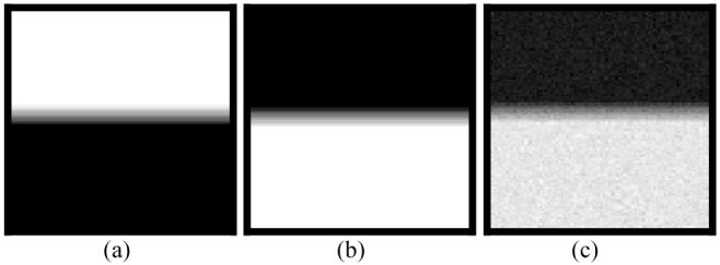
Simulation of a phantom image of two density levels with PVE. Picture (a) represents the distribution of {Z_i1} for tissue type 1. Pixels in the upper (white) region are fully filled with tissue type 1, while pixels in the lower (black) region have zero percentage of tissue type 1. Picture (b) reflects the distribution of {Z_i2} for tissue type 2. Pixels in the upper (black) region have zero percentage of tissue type 2, while pixels in the lower (white) region are fully filled by tissue type 2. The PVE occurs between the white and black regions of ten-pixel width in the middle. Picture (c) shows the two-tissue phantom image with Gaussian noise.

A.2. Implementation of Equations (20) and (21)

The MAP-EM algorithm of (18)-(19) with quadratic approximation of (21) was implemented by directly programming these three equations using C++ language. When implementing the algorithm with the mathematically exact formula of (20), we employed the QR program (C++ code) in [23] to solve the fifth-order equation while equations (18) and (19) were directly programmed using C++ language as described above. These source codes were complied in a Visual C++ environment on a HP XW8000 PC platform (2.4 GHz CPU and 2.0 GB RAM). The complied programs with equation (20) (or theoretically exact implementation) and equation (21) (or quadratic approximated implementation) each ran up to 60 iterations to ensure that a stable solution is achieved. In our experiments below, a stable solution was observed after ten iterations.

A.3. Convergence Comparison between Equations (20) and (21)

The convergence performance of the MAP-EM algorithm using equations (20) and (21) respectively was studied by the measure of the relative error

$$\epsilon \left(Z_{ik}\right)=\frac{\sum _{i=1}^{I_R}\mid Z_{ik}^{\left(n\right)}-Z_{ik}^{\left(\text{truth}\right)}\mid }{I_R},$$ (22)

where I_R indicates the number of those pixels inside the PV horizontal strip in Figure 1. Figure 2 shows, as an example, the result when the initial $\left\{Z_{ik}^{\left(0\right)}\right\}$ had 50% deviation from the ground truth. Similar results were observed for other initial errors from 10% up to 90% on $\left\{Z_{ik}^{\left(0\right)}\right\}$. A stable solution after ten iterations was observed. The computing time for the iterative process was documented and plotted in Figure 3. The QR program for the solution of (20) costs approximately 25% more computing time than the computation of (21) after 30 iterations.

Fig. 2.

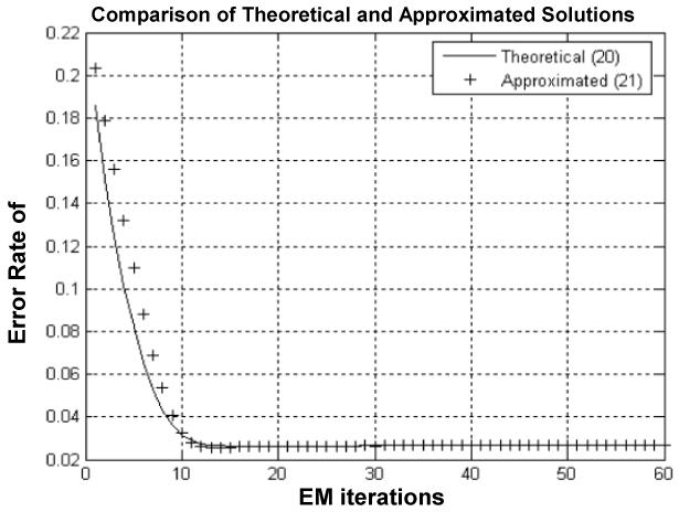
Comparison of iterated tissue mixture percentages against iteration number using the theoretical solution (20) (solid line) and the approximated solution (21) (crosses), where β =0.5 was used. A similar convergence rate was observed for both Z_i1 and Z_i2 because of the condition (7), i.e., Z_i2 = 1-Z_i1 .

Fig. 3.

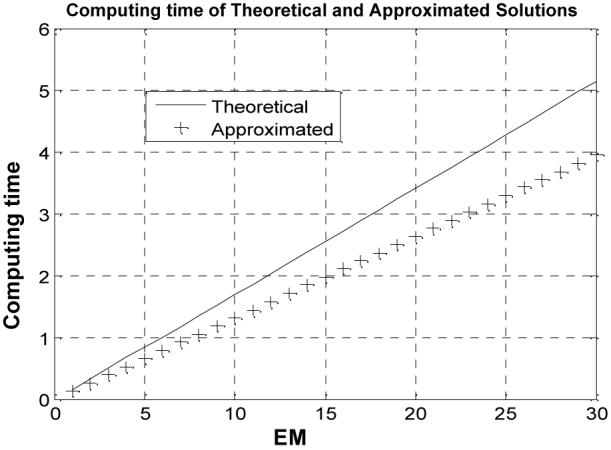
Comparison of computing time (seconds) against iteration number between the theoretical solution (20) (solid line) and the approximated solution (21) (crosses), where β =0.5 was used

A.4. Estimation of Tissue Model Parameters {μ_k ,ν_k}

We first studied the accuracy of estimators (18) and (19) with known {Z_ik}. By setting the initial model parameters $\{{\mu }_k^{\left(0\right)},{\nu }_k^{\left(0\right)}\}$ with 99.9% error from the ground truth of {μ₁=100, ν₁=100, μ₂=500, ν₂=300} and fixing the mixture percentages $\left\{Z_{ik}^{\left(n\right)}\right\}$ as the ground truth of Figure 1(a) and Figure 1(b) at all iterations, we obtained the iterated results after thirty iterations $\{{\mu }_k^{\left(30\right)},{\nu }_k^{\left(30\right)}\}$ as shown in Table 1, where the model parameters of the phantom image were computed over those pixels inside the white and black regions in Figure 1(c) excluding the PVE (i.e., ignoring the grey strip in the middle). These results indicate that the phantom image with Gaussian noise is accurately simulated, and the estimation of the model parameters is robust regardless of 99.9% initial error.

TABLE 1.

Iterated tissue model parameters by the MAP-EM algorithm with comparison to that of the phantom image. β was set to zero to ignore the effect of the penalty

	μ 1	μ 2	ν 1	ν 2
Result from the phantom image	100.08	500.04	99.60	296.62
Iterated result with fixed Zik	100.07	500.02	99.47	297.35

We then repeated the above experiment by updating the mixture percentages $\left\{Z_{ik}^{(n+1)}\right\}$ with equation (20) and (21) respectively from the initial of $\left\{Z_{ik}^{\left(0\right)}\right\}$ being the ground truth. The iterated results after thirty iterations are shown in Table 2. The % error reflects the difference of the iterated result from the corresponding ground truth. The updates by equations (20) and (21) generated similar results. There is some difference in the estimate of ν₁ due to a smaller mean and larger variance for tissue type 1 in the phantom image, as compared to that of tissue type 2. This difference was observed in all the experiments performed in this study.

TABLE 2.

Comparison of iterated tissue model parameters using the theoretical solution (20) and the approximated solution (21). β was set to zero to ignore the effect of the penalty

	ERR(μ1)	ERR(μ2)	ERR(ν1)	ERR(ν2)
Theoretical (20)	0.05%	0.00%	1.41%	2.18%
Approximated (21)	0.05%	0.00%	0.89%	2.24%

A.5. Performance Comparison between Equations (20) and (21)

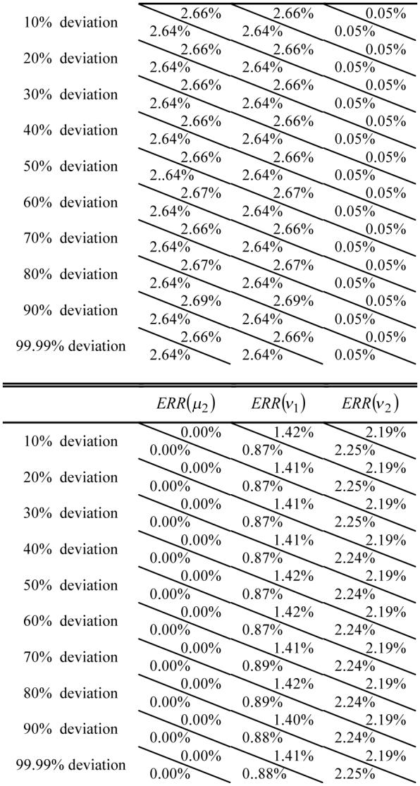
To show the robustness of the MAP-EM segmentation algorithm for different initial estimates on the mixture percentages, we repeated the above experiment by allowing the initial $\left\{Z_{ik}^{\left(0\right)}\right\}$ with various % deviations from 10% up to 99.9%. The % deviations were generated by sampling each $Z_{ik}^{\left(0\right)}$ using the Gaussian noise generator [23] with a given % standard deviation from its ground truth Z_ik in Figure 1. The iterated results after thirty iterations are shown in Table 3. The value in the upper right corner of each cell was from the theoretically exact solution (20), while the value in the lower left corner of each cell was from the quadratic approximated solution (21). The percentage error of estimating the tissue mixture percentages {Z_ik} in the table was computed from those pixels in the PV horizontal strip in Figure 1. Because of the penalty, the percentages {Z_ik} in the white and black regions of Figure 1 were accurately estimated. Both implementations with exact solution (20) and approximated solution (21) generated similar results. Some difference in estimating the variance of tissue type 1 {ν₁} was observed and explained before.

TABLE 3.

Comparison of iterated tissue model parameters and tissue mixture percentages using the theoretical solution (20) (upper corner in each cell) and the approximated solution (21) (lower corner in each cell), whereb β =0.5 was used

B. Further Simulation Studies for K=3

A three-tissue phantom image of 256×256 array size was generated following the same procedure as described in Section III.A.1 above for Figure 1. Tissue type 1 had a mean value of μ₁=230 units and variance of ν₁=180 units. Its percentage distribution {Z_i1} across the FOV is shown in Figure 4(a). A PV strip of 10 pixel unit width is present vertically and horizontally, respectively, between the white (Z_i1=1) and black (Z_i1=0) regions. A noise image {X_i1} of tissue type 1 was simulated with Gaussian noise, where the image density X_i1 at pixel i was given by a Gaussian noise generator [23] with mean of ${\stackrel{‒}{X}}_{i1}=Z_{i1}{\mu }_1$ and variance of ${\sigma }_{i1}^2=Z_{i1}{\nu }_1$. Tissue type 2 had a mean value of μ₂=500 units and variance of ν₂=300 units. Its percentage distribution {Z_i2} across the FOV is shown in Figure 4(b). A noise image {X_i2} of tissue type 2 was simulated with Gaussian noise by the same procedure as simulating the noise image of tissue type 1 above. Tissue type 3 had a mean value of μ₂=800 units and variance of ν₂=500 units. Its percentage distribution {Z_i3} across the FOV is shown in Figure 4(c). A vertical PV strip of 10 pixel unit width is present between the black (Z_i3=0) region on the left and the white (Z_i3=1) region on the right. A noise image {X_i3} of tissue type 3 was simulated with Gaussian noise by the same procedure as simulating the noise image of tissue type 1 above. Adding these three noise images together results in the observable noise image {Y_i}, which is shown in Figure 4(d).

Fig. 4.

Simulation of a phantom image of three density levels with PVE. Picture (a) represents the distribution of {Z_i1} for tissue type 1. Picture (b) reflects the distribution of {Z_i2} for tissue type 2. Picture (c) shows the distribution of {Z_i3} for tissue type 3. The PVE occurs between the white and black regions of ten-pixel width in the three pictures. Picture (d) shows the three-tissue phantom image with Gaussian noise, where the center square area of ten-pixel width contains three tissue types and the horizontal and vertical strips of ten-pixel width contains two tissue types.

The update of the tissue model parameters {μ_k ,ν_k} was performed by equations (18) and (19) with 99.9% initial error, i.e., the same as the initial estimation in K=2. Various initial errors from 10% to 99.9% were selected for the tissue mixture percentages $\left\{Z_{ik}^{\left(0\right)}\right\}$ relative to the ground truth in the pictures of Figure 4. The initial tissue percentages were updated by both the theoretical solution of (A.7)-(A.8) and the quadratic approximation (A.9)-(A.10). Since the QR program in [23] is valid only for a single equation of (20), not a set of more than one equation of high orders, we adapted the Newton’s gradient program [23] to solve the set of two fifth-order equations (A.7)-(A.8). The linear equations (A.9)-(A.10) were coded directly by C++ language. Both the Newton’s program and C++ code of (A.9)-(A.10) were complied and executed by the same computer as described in Section III.A.2 above. The results after 30 iterations are shown in Table 4 for 50% initial error. The percentage error of estimating the tissue mixture percentages {Z_ik} in the table was computed from those pixels, which contain three tissue types, in the PV square area in the center of Figure 4(d). Both the theoretical solution and the quadratic approximation generated similar estimates of the tissue model parameters and the tissue mixture percentages, the same observation as seen in the study for K=2.

TABLE 4.

Comparison of iterated tissue model parameters and tissue mixture percentages using the theoretical solution (A.7)-(A.8) and the approximated solution (A.9)-(A.10)

	{Zi1}	{Zi2}	{Zi3}	μ 1	μ 2	μ 3	ν 1	ν 2	ν 3
Theoretical	1.30%	3.16%	1.96%	0.03%	0.01%	0.02%	0.15%	1.53%	0.96%
Approximated	1.33%	3.04%	1.86%	0.03%	0.01%	0.02%	0.16%	1.52%	0.95%

The convergence performance of the MAP-EM algorithm using the theoretical solution (A.7)-(A.8) and the quadratic approximation (A.9)-(A.10) respectively is compared in Figure 5. Equation (22) was used, here I_R now indicates the number of those pixels inside the PV square region of three tissue types in the center of Figure 4(d). A stable solution after 40 iterations was observed. A faster convergence for a tissue type of smaller mean and variance was noted. A larger number of iteration is needed for pixels containing more tissue types. The computing time for the iterative process was documented and plotted in Figure 6. The Newton’s gradient program for solving the fifth-order equations (A.7)-(A.8) has the same efficiency in computation compared to directly solving the linear equations (A.9)-(A.10).

Fig. 5.

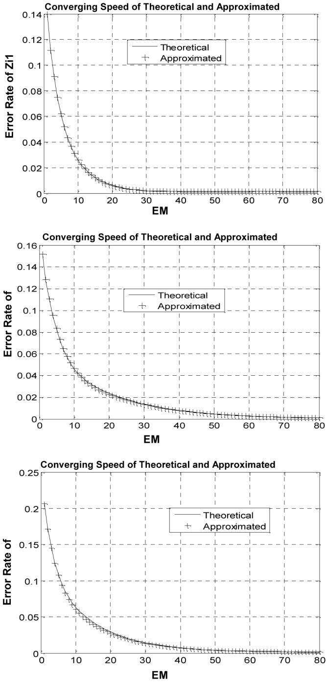
Comparison of iterated tissue mixture percentages against iteration number using the theoretical solution (solid line) and the approximated solution (crosses). Top one reflects the error rate of Z_i1, middle one reflects the error rate of Z_i2 , and bottom one shows the error rate of Z_i3

Fig. 6.

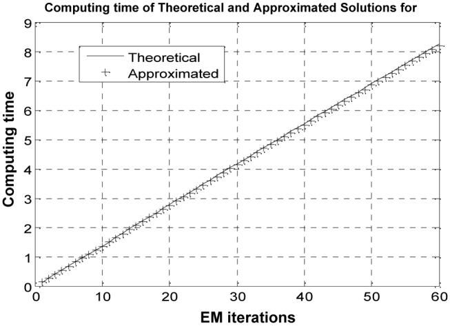
Comparison of computing time (seconds) against iteration number between the theoretical solution (solid line) and the approximated solution (crosses)

IV. Digital brain MRI phantom study

A. Brain MRI Phantom Simulation

A more realistic MRI brain digital phantom was simulated via the anatomical model available at the BrainWeb:http://www.bic.mni.mcgill.ca/brainweb/, which consists of a set of three-dimensional (3D) “fuzzy” tissue membership volumes, one for each tissue type (e.g., cerebrospinal fluid (CSF), grey matter, white matter, etc). Since the voxel values in these volumes reflect the proportions of the tissues present in the voxels in the range of [0, 1], it is straightforward to obtain the tissue mixture distribution {Z_ik} for each tissue type k for the PV model of (5)-(9). For the purpose of this study, a noise-free 3D image volume was firstly simulated using the T1 sequence of the MRI simulator provided at the BrainWeb, where only those voxels labeled as CSF, grey matter and white matter were extracted because of their dominating contribution to the phantom. Then the statistical mean associated with each of the three tissue types, denoted by {μ₁, μ₂, μ₃}, was computed by referring to {Z_ik}. For each voxel i to be simulated, three independent Gaussian random variables of mean Z_ikμ_k and variance Z_ikν_k corresponding to the three tissue types were generated individually and summed together, where {ν₁ ,ν₂ ,ν₃} were user-defined tissue variances, reflecting different noise levels. Based on the above arguments, a digital MRI brain phantom of size 181×217×181, consisting of three tissue types, CSF, grey matter and white matter, was simulated and its 82^nd slice is shown in Figure 7(a). The associated parameter sets of means and variances are listed in Table 5.

Fig. 7.

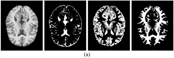
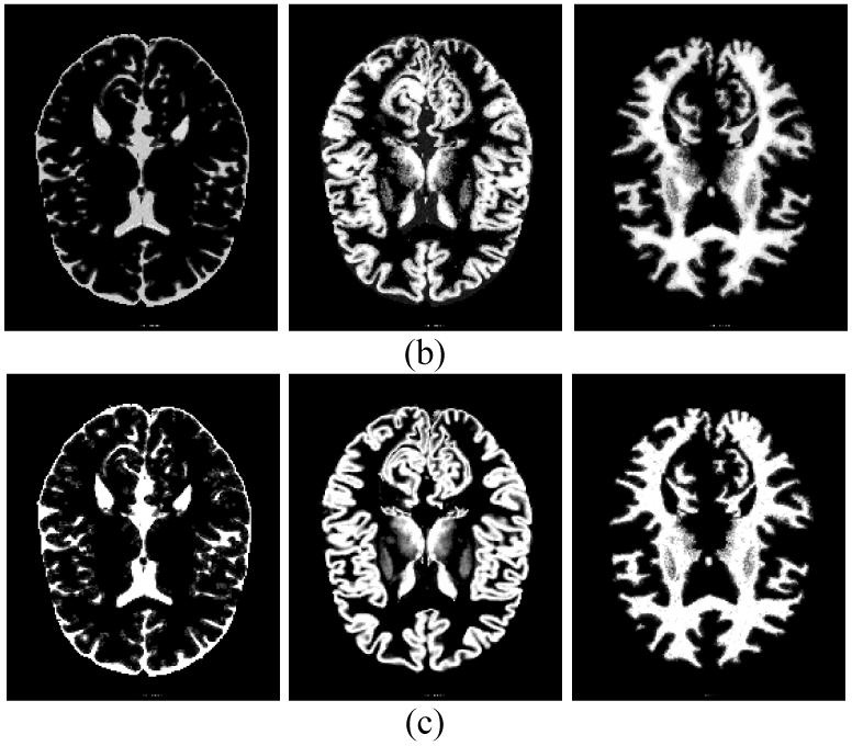
Simulated MRI brain phantom: (a) from left to right, they are noise phantom image at the 82^nd slice, ground truth of {Z_i1} for CSF, ground truth {Z_i2} for grey matter, and ground truth {Z_i3} for white matter respectively, (b) estimated {Z_ik} by the theoretical MAP-EM solution, and (c) estimated {Z_ik} by the approximated MAP-EM solution.

TABLE 5.

Ground truth of the simulated brain MRI phantom

Phantom dimension	181×217×181
CSF statistics	μ1 = 47 , ν1 = 5
Grey matter statistics	μ2 = 111 , ν2 = 20
White matter statistics	μ3 = 149 , ν3 = 30

B. Estimation of Tissue Model Parameters, Given Ground Truth as Initial

In this section, the ground truth of {μ_k ,ν_k} for CSF, grey matter and white matter, as well as {Z_ik} for each voxel were given as initial values of $\{Z_{ik}^{\left(0\right)},{\mu }_k^{\left(0\right)},{\nu }_k^{\left(0\right)}\}$ and the MAP-EM algorithm was run up to 100 iterations to ensure a stable estimation is achieved. For comparison purpose, both theoretical and approximated solutions as outlined by equations (20) and (21) were implemented and the results are tabulated Table 6. Both solutions have a similar performance in parameter estimation.

TABLE 6.

Parameter estimation by both theoretical and approximated MAP-EM solutions, given the ground truth as initials

	Theoretical	Approximated
Error rate of {Zi1}	0.93%	1.48%
Error rate of {Zi2 }	2.27%	2.17%
Error rate of {Zi3 }	3.13%	3.56%
Mean of CSF	46	46
Mean of grey matter	110	111
Mean of white matter	148	149
Variance of CSF	4	6
Variance of grey matter	14	19
Variance of white matter	22	27

C. Estimation of Tissue Model Parameters, Given Deviated Initials

Different from Section IV.B above where $\{Z_{ik}^{\left(0\right)},{\mu }_k^{\left(0\right)},{\nu }_k^{\left(0\right)}\}$ were initialized as the ground truth values, a more practical initialization strategy was taken in this section. Though the resulting $\{Z_{ik}^{\left(0\right)},{\mu }_k^{\left(0\right)},{\nu }_k^{\left(0\right)}\}$ would have certain deviations from their true values, this initialization strategy is considered to be more realistic, and can be summarized into the following steps.

1. According to the histogram of the synthetic MRI brain phantom, each voxel i was pre-assigned a discrete label from {1, 2, 3}, representing CSF, grey matter and white matter respectively via a thresholding operation, denoted by L_i, L_i ∈ {1, 2, 3}.

2. Based on {L_i}, $\{{\mu }_k^{\left(0\right)},{\nu }_k^{\left(0\right)}\}$ were calculated by grouping voxels which belong to the same labeled class. Although $\{{\mu }_k^{\left(0\right)},{\nu }_k^{\left(0\right)}\}$ obtained in this way could not exactly reflect the true statistical properties, especially for $\left\{{\nu }_k^{\left(0\right)}\right\}$, they could be refined after sufficient EM iterations steered by {Z_ik} which is the most impacting factor.

3. The final and crucial step is to initialize $\left\{Z_{ik}^{\left(0\right)}\right\}$. For each voxel i, the number of contributing tissue types {N_i} alternatively determined via its 6-connected neighbors in 3D image domain. Figure 8 illustrates such initialization process in the case of 2D image space where “C”, “G” and “W” represent CSF, grey matter and white matter respectively.

Once {N_i} have been determined for each voxel, $\left\{Z_{ik}^{\left(0\right)}\right\}$ were accordingly initialized in such a way that if N_i = 2, i.e., voxel i contains a mixture of CSF and grey matter for example, then $Z_{i1}^{\left(0\right)}=0.5$, $Z_{i2}^{\left(0\right)}=0.5$ and $Z_{i3}^{\left(0\right)}=0$. For the case of N_i = 3, then $Z_{i1}^{\left(0\right)}=0.33$, $Z_{i2}^{\left(0\right)}=0.33$, and $Z_{i3}^{\left(0\right)}=0.34$.

Fig. 8.

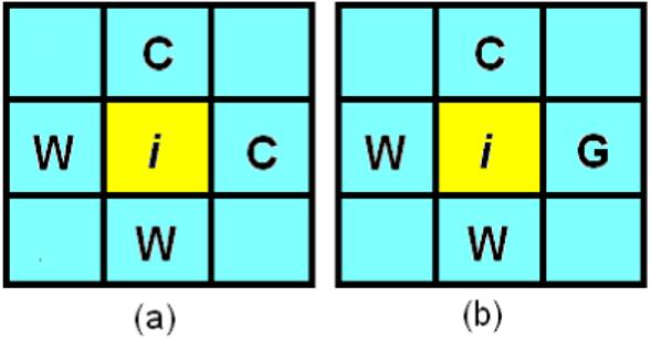
Two-dimensional illustration of how to determine the number of contributing tissue types inside each pixel, (a) pixel i is mixed by two tissue types: CSF and white matter; and (b) pixel i is mixed by three tissue types: CSF, white matter and grey matter.

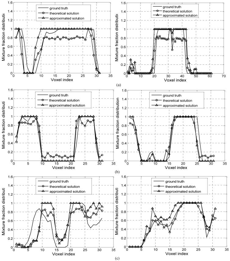
The estimated model parameters {μ_k ,ν_k} and tissue mixture components {Z_ik} after 100 EM iterations by the MAP-EM algorithm with both theoretical and approximated solutions are summarized in Table 7, and the distribution maps of {Z_ik} in the 82^nd slice corresponding to each tissue type are shown in Figure 7(b-c) respectively. For visual judgment, the profiles of CSF, grey matter and white matter along both vertical and horizontal directions by sampling a one-pixel-wide stripe on Figure 7(b-c) are shown in Figure 9(a-c).

TABLE 7.

Parameter estimation by both theoretical and approximated MAP-EM solutions using the new initialization strategy

	Theoretical	Approximated
Error rate of {Zi1}	6.79%	4.68%
Error rate of {Zi2 }	9.60%	7.12%
Error rate of {Zi3 }	9.67%	9.97%
Mean of CSF	31	40
Mean of grey matter	109	112
Mean of white matter	151	149
Variance of CSF	13	6
Variance of grey matter	28	13
Variance of white matter	26	28

Fig. 9.

Profiles of CSF (a), grey matter (b) and white matter (c) along vertical (left) and horizontal (right) directions drawn from Figure 7(b-c) for visual evaluation.

Both solutions showed some different performances in parameter estimation for mixed cases of K=2 and K=3 across the FOV when the initials $\{Z_{ik}^{\left(0\right)},{\mu }_k^{\left(0\right)},{\nu }_k^{\left(0\right)}\}$ were estimated from the acquired image data. In light of the numerical simulation studies above where the cases of K=2 and K=3 are known across the FOV, the different performances of the two solutions for mixed cases of K=2 and K=3 across the FOV are likely due to the determination of the number of tissue types in a voxel from the current iteration for the next iteration. The theoretical solution uses the QR program for voxels containing two tissue types (K=2) and the Newton’s gradient program for voxels containing three tissue types (K=3). The approximated solution applies the same strategy for the set of linear equations (A.9)-(A.10) for any K value. The following investigations will provide more insights on the difference.

D. Computational Analysis

In this section, the theoretical and approximated solutions were compared from two aspects: (1) converging speed and (2) computing time.

D.1. Converging Speed

The model parameters {μ_k ,ν_k} are usually converging to a stable estimate in less iterations than the mixture percentages {Z_ik} do. So we report the converging speed of {Z_ik} as iteration number goes up. Curves describing how the error rate of {Z_ik} varies along the EM iterations for each tissue type k are shown in Figure 10. Since the constraint of Z_i1 + Z_i2 + Z_i3 =1 leads to two degrees of freedom and, therefore, only the changes of {Z_ik} associated with CSF and grey matter were plotted. The theoretical solution converged to a stable estimate in less iteration number and had a slightly larger relative error defined by (22), compared to the approximated solution.

Fig. 10.

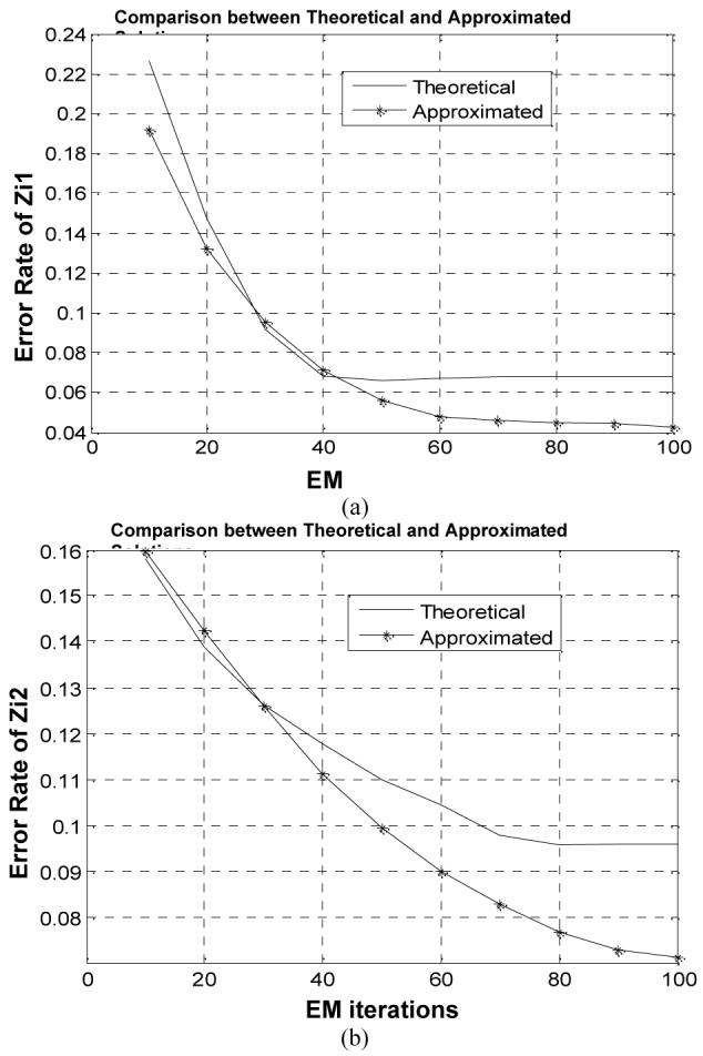
Error rate of {z_ik} decreases as the EM iteration number increases. (a) plot shows the changes of {z_ik} associated with CSF by the theoretical and approximated MAP-EM solutions, and (b) plot shows the changes of {Z_ik} associated with grey matter (GM) by the theoretical and approximated MAP-EM solutions.

D.2. Computing Time

The computing time of the theoretical and approximated MAP-EM solutions for segmenting the 3D MRI brain phantom image of 181×217×181 array size is shown in Figure 11 in unit of seconds as the iteration goes up. The computing time of the theoretical MAP-EM solution is almost five times more than that of the approximated solution for an equivalent EM iteration.

Fig. 11.

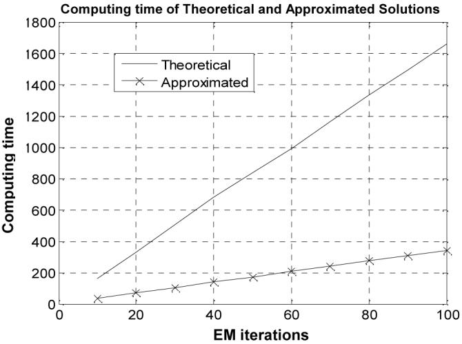
Comparison of computing time (seconds) against iteration number between the theoretical solution and the approximated solution for the MRI brain phantom study.

Comparing Figure 3 and Figure 6 to Figure 11 in terms of computing time for segmenting the corresponding 2D numerical and 3D MRI brain phantoms respectively, it can be seen that the number of voxels containing two tissue types is much larger than the number of voxels containing three tissue types in the 3D MRI brain image. This is because that the theoretical solution consumes more computing time for K=2 than the approximated solution at an equivalent iteration. In clinical applications, we expect to have more voxels containing two tissue types than voxels containing three or more tissue types and, therefore, the approximated solution may have an advantage over the theoretical solution in computing efficiency. By the results of Table 7 and Figure 9, both the approximated solution and the theoretical solution have a similar performance in estimating model parameters and mixture percentages of the three tissue types in the 3D MRI brain image.

V. discussion and Conclusion

In the mathematical derivation of the MAP-EM algorithm, we assumed K to be the total number of different tissue types inside the body. The tissue model parameters {μ_k ,ν_k} of these K tissue types were estimated using all the image data {Y_i} by (18) and (19). In the implementation of (20) and (21) for estimation of the tissue mixture percentages {Z_ik}, only datum Y_i and its neighbors were used. Then the number of tissue types in each voxel varied across the FOV. In other words, the total number of tissue types K inside the body can be much greater than two, while the estimators (20) and (21) remain valid if a voxel contains no more than two tissue types. Similarly, estimators of (A.7)-(A.8) and (A.9)-(A.10) in Appendix are still valid if a voxel contains no more than three tissue types, despite the total number of tissue types in the body is far beyond three. This was demonstrated by clinical studies in segmenting patient abdominal CT images for virtual colonoscopy application [20].

Estimator (20) is mathematically exact. It is a fifth-order equation and would generate five possible values for each Z_i1 when the QR program in [23] is used. In most cases, the constraint of 0 ≤ Z_i1 ≤ 1 eliminated the other four possible values. Sometimes we encountered a choice of one from two possible values for Z_i1 in the range of [0, 1]. In these cases, we chose the one which was closer to the previously iterated value. In contrast, equation (21) determines a value for each Z_i1 in the range of [0, 1]. However, because the quadratic approximation is made at the n-th iteration, then the estimator (21) for {Z_i1} at the (n+1)th iteration is somehow bounded to the result at the n-th iteration, causing a slower initial convergence compared to the theoretical solution (20) (see Figure 2 and Figure 10). For K>2, the QR program is no longer applicable. When the Newton gradient program in [23] was used, a same convergence speed was obtained as that of the quadratic approximation (see Figure 5). This is because of the Newton gradient program searches the solution from the n-th iterated result, a similar bound to the n-th iteration as that in the quadratic approximation. For digital implementation of both theoretical solution and quadratic approximation, we modified the condition 0 ≤ Z_i1 ≤ 1 to be 0.01 ≤ Z_i1 ≤ 0.99 to avoid Z_ik being zero (or avoid numerical instability when Z_ik is in the denominator).

Both estimators of the theoretical solution and the quadratic approximation generated similar results for the tissue mixture percentages {Z_ik}, leading to a similar estimate of the tissue model parameters {μ_k ,ν_k} by equations (18) and (19). The computational efficiency was also similar for both estimators when the Newton’s gradient program was used to solve the set of fifth-order equations for the theoretical solution. There is no noticeable benefit to solve a set of fifth-order equations for the tissue mixture percentages (e.g., equations (A.7) and (A.8) in Appendix), as compared to solving a set of linear equations by the quadratic approximation (e.g., equations (A.9) and (A.10) in Appendix), unless a more accurate program, similar to or better than the QR program, is available to solve the fifth-order equations. Therefore, the quadratic approximation may be a choice for practical applications at present time.

Further validation of the algorithm by clinical studies is needed and is currently under investigation for CT colonoscopy application [20], where several practical issues regarding the MAP-EM implementation (e.g., initialization procedure, neighboring system optimization for increase or decrease of the number of tissue types at a concerned voxel, iteration speedup, recovery of submerged polyps inside tagged colonic materials, etc.) were studied. The whole implementation pipeline including post-segmentation strategies for removal of tagged colonic materials and extraction of mucosa layer from the MAP-EM segmentation was comprehensively evaluated by 52 patient CTC studies, which were downloaded from the website of the Virtual Colonoscopy Screening Resource Center, by two well-trained and experienced radiologists.

Appendix

This section provides the derivation for solution of {$\left\{Z_{ik}^{(n+1)}\right\}$} by setting the partial derivative of Q(ϴ | ϴ⁽ⁿ⁾) with respect to Z_ik to zero under the conditions (7). Equation (15) can be rewritten as

$$Q(ϴ\mid {ϴ}^{\left(n\right)})=-\frac{1}{2}\sum _{i=1}^I\sum _{k=1}^K{Q}_{i,k}\left(Z_{ik}\right),$$ (A.1)

where the energy function on the neighborhood of voxel i in the conditional expectation term Q_i,k (Z_ik ) at the n-th iteration is understood as

$$U\left(Z_{ik}\right)=\sum _{r\in {\epsilon }_i}{w}_{ir}{(Z_{ik}-Z_{rk}^{\left(n\right)})}^2,$$ (A.2)

For K=1, Z_i1 =1 from the conditions (7), and Q(ϴ | ϴ⁽ⁿ⁾) is independent from Z_i1 and, therefore, the partial derivative of Q(ϴ | ϴ⁽ⁿ⁾) with respect to Z_i1 is zero for all voxels. This is expected. In this case, the mean and variance estimates by (18) and (19) become

$${\mu }_1=\frac{1}{I}\sum _{i=1}^I{Y}_i,{\nu }_1=\frac{1}{I}\sum _{i=1}^I{(Y_i-{\mu }_1)}^2,$$ (A.3)

These estimates are also expected for an image consisting of a single tissue type. For K=2, we have

$$Q(ϴ\mid {ϴ}^{\left(n\right)})=-\frac{1}{2}\sum _{i=1}^I\{Q_{i,1}\left(Z_{i1}\right)+Q_{i,2}(1-Z_{i1})\},$$ (A.4)

By setting the partial derivative of Q(ϴ | ϴ⁽ⁿ⁾) with respect to Z_i1 to zero, we had obtained equation (20). By the quadratic approximation mentioned before, equation (A.4) becomes

$$Q(ϴ\mid {ϴ}^{\left(n\right)})=-\frac{1}{2}\sum _{i,k}\left\{\ln \left(2\pi \right)+\ln \left({\sigma }_{ik}^{\left(n\right)}\right)+\frac{1}{{\sigma }_{ik}^{\left(n\right)}}[{\left(X_{ik}^2\right)}^{\left(n\right)}-2X_{ik}^{\left(n\right)}{Z}_{ik}{\mu }_k+Z_{ik}^2{\mu }_k^2]+\beta U\left(Z_{ik}\right)\right\},$$ (A.5)

By setting the partial derivative of Q(ϴ | ϴ⁽ⁿ⁾) with respect to Z_i1 to zero, we had obtained equation (21). For a special case of $Y_i={\mu }_1^{\left(n\right)}$ or $Y_i={\mu }_2^{\left(n\right)}$ and ignoring the penalty term, equation (21) converges to a stable solution of $Z_{ik}^{(n+1)}=Z_{ik}^{\left(n\right)}$. For k=3, we have

$$Q(ϴ\mid {ϴ}^{\left(n\right)})=-\frac{1}{2}\sum _{i=1}^I\{Q_{i,1}\left(Z_{i1}\right)+Q_{i,2}\left(Z_{i2}\right)+Q_{i,3}(1-Z_{i1}-Z_{i2})\},$$ (A.6)

By setting the partial derivative of Q(ϴ | ϴ⁽ⁿ⁾) with respect to Z_i1 and Z_i2 respectively to zero, we can obtain two fifth-order equations for the solutions of $Z_{i1}^{(n+1)}$ and $Z_{i2}^{(n+1)}$,

$$\begin{array}{cc}\hfill & a_1{\xi }_1^5+b_1{\xi }_1^4+c_1{\xi }_1^3+d_1{\xi }_1^2+e_1{\xi }_1^1+f_1{\xi }_1^4{\xi }_2^1+g_1{\xi }_1^3{\xi }_2^2\hfill \\ \hfill & +h_1{\xi }_1^3{\xi }_2^1+o_1{\xi }_1^2{\xi }_2^3+p_1{\xi }_1^2{\xi }_2^2+q_1{\xi }_1^2{\xi }_2^1+r_1{\xi }_1^1{\xi }_2^2\hfill \\ \hfill & +s_1{\xi }_1^1{\xi }_2^1+t_1{\xi }_2^2+t_1{\xi }_2^1+{\eta }_1=0\hfill \end{array}$$ (A.7)

$$\begin{array}{cc}\hfill & a_2{\xi }_2^5+b_2{\xi }_2^4+c_2{\xi }_2^3+d_2{\xi }_2^2+e_2{\xi }_2^1+f_2{\xi }_2^4{\xi }_1^1+g_2{\xi }_2^3{\xi }_1^2\hfill \\ \hfill & +h_2{\xi }_2^3{\xi }_1^1+o_2{\xi }_2^2{\xi }_1^3+p_2{\xi }_2^2{\xi }_1^2+q_2{\xi }_2^2{\xi }_1^1+r_2{\xi }_2^1{\xi }_1^2\hfill \\ \hfill & +s_2{\xi }_2^1{\xi }_1^1+t_2{\xi }_1^2+{\tau }_2{\xi }_1^1+{\eta }_2=0\hfill \end{array}$$ (A.8)

where ${\xi }_1=Z_{i1}^{(n+1)}$, ${\xi }_2=Z_{i2}^{(n+1)}$, and all the coefficients have been determined by the results at the n-th iteration. By the quadratic approximation (A.5) and setting the partial derivative of Q(ϴ | ϴ⁽ⁿ⁾) with respect to Z_i1 and Z_i2 respectively to zero, we have two linear equations of

$$A_1{Z}_{i1}^{(n+1)}+B_1{Z}_{i2}^{(n+1)}+C_1=0,$$ (A.9)

$$A_2{Z}_{i1}^{(n+1)}+B_2{Z}_{i2}^{(n+1)}+C_2=0,$$ (A.10)

where the coefficients A_i, B_i, and C_i have been determined by the results at the n-th iteration.

For K=4, we can derive three fifth-order equations, similar to (A.7)-(A.8), to estimate Z_i1, Z_i2 and Z_i3 with Z_i4 = 1 - Z_i1 - Z_i2 - Z_i3. By the quadratic approximation, we can derive three linear equations, similar to (A.9)-(A.10), to estimate Z_i1, Z_i2 and Z_i3 with Z_i4 = 1 - Z_i1 - Z_i2 - Z_i3. In general cases of K tissue types, we can derive theoretically K-1 equations under conditions (7) to estimate the K tissue mixture percentages in each voxel. In practice, there are very few cases where K goes beyond 4.

References

- [1].Li L, Lu H, Li X, Huang W, Tudorica A, Christodoulou C, Krupp L, Liang Z. MRI volumetric analysis of multiple sclerosis: Methodology and validation. IEEE Transactions on Nuclear Science. 2003;50(5):1686–1692. [Google Scholar]
- [2].Liang Z, Jaszczak R, Coleman E. Parameter estimation of finite mixtures using the EM algorithm and information criteria with application to medical image processing. IEEE Transactions on Nuclear Science. 1992;39(4):1126–1133. [Google Scholar]
- [3].Sanjay-Gopal S, Hebert T. Bayesian pixel classification using spatially variant finite mixtures and the generalized EM algorithm. IEEE Transactions on Image Processing. 1998;7(7):1014–1028. doi: 10.1109/83.701161. [DOI] [PubMed] [Google Scholar]
- [4].Zhang Y, Brady M, Smith S. Segmentation of brain MR images through a hidden Markov random field model and the expectation-maximization algorithm. IEEE Transactions on Medical Imaging. 2001;20(1):45–57. doi: 10.1109/42.906424. [DOI] [PubMed] [Google Scholar]
- [5].Pham D, Prince J. Adaptive fuzzy segmentation of magnetic resonance images. IEEE Transactions on Medical Imaging. 1999;18(9):737–752. doi: 10.1109/42.802752. [DOI] [PubMed] [Google Scholar]
- [6].Li X, Li L, Lu H, Liang Z. A partial volume segmentation of brain magnetic resonance images based on maximum a posteriori probability. Medical Physics. 2005;32(7):2337–2345. doi: 10.1118/1.1944912. [DOI] [PMC free article] [PubMed] [Google Scholar]
- [7].Choi H, Haynor D, Kim Y. Partial volume tissue classification of multi-channel magnetic resonance images - A mixel model. IEEE Transactions on Medical Imaging. 1991;10(3):395–407. doi: 10.1109/42.97590. [DOI] [PubMed] [Google Scholar]
- [8].Santago P, Gage H. Quantification of MR brain images by mixture density and partial volume modeling. IEEE Transactions on Medical Imaging. 1993;12(3):566–574. doi: 10.1109/42.241885. [DOI] [PubMed] [Google Scholar]
- [9].Santago P, Gage H. Statistical models of partial volume effect. IEEE Transactions on Image Processing. 1995;4(11):1531–1539. doi: 10.1109/83.469934. [DOI] [PubMed] [Google Scholar]
- [10].Laidlaw D, Fleischer K, Barr A. Partial-volume Bayesian classification of material mixture in MR volume data using voxel histograms. IEEE Transactions on Medical Imaging. 1998;17(1):74–86. doi: 10.1109/42.668696. [DOI] [PubMed] [Google Scholar]
- [11].Blekas K, Likas A, Galatsanos N, Lagaris I. A spatially constrained mixture model for image segmentation. IEEE Transactions on Neural Networks. 2005;16(4):494–498. doi: 10.1109/TNN.2004.841773. [DOI] [PubMed] [Google Scholar]
- [12].Leemput K, Maes F, Vandermeulen D, Suetens P. A unifying framework for partial volume segmentation of brain MR images. IEEE Transactions on Medical Imaging. 2003;22(1):105–119. doi: 10.1109/TMI.2002.806587. [DOI] [PubMed] [Google Scholar]
- [13].Lei T, Sewchand W. Statistical approach to X-ray CT imaging and its applications in image analysis - Part I and II. IEEE Transactions on Medical Imaging. 1992;11(1):53–69. doi: 10.1109/42.126910. [DOI] [PubMed] [Google Scholar]
- [14].Fuderer M. The information content of MR images. IEEE Transactions on Medical Imaging. 1988;7(4):368–380. doi: 10.1109/42.14521. [DOI] [PubMed] [Google Scholar]
- [15].Macovski A. Noise in MRI. Magnetic Resonance in Medicine. 1996;36(4):494–497. doi: 10.1002/mrm.1910360327. [DOI] [PubMed] [Google Scholar]
- [16].Li X, Eremina D, Li L, Liang Z. Partial volume segmentation of medical images; Conference Record of IEEE Nuclear Science Society-Medical Imaging Conference; Portland, Oregon, USA. November 19-26, 2003; in CD-ROM. [Google Scholar]
- [17].Dempster A, Laird N, Rubin D. Maximum likelihood from incomplete data via the EM algorithm. Journal of the Royal Statistics Society. 1977;39(B):1–38. [Google Scholar]
- [18].Leemput K, Maes F, Vandermeulen D, Suetens P. Automated model-based tissue classification of MR images of the brain. IEEE Transactions on Medical Imaging. 1999;18(10):897–908. doi: 10.1109/42.811270. [DOI] [PubMed] [Google Scholar]
- [19].Geman S, Geman D. Stochastic relaxation, Gibbs distributions, and the Bayesian restoration of images. IEEE Transactions on Pattern Analysis and Machine Intellengence. 1984 Jun;PAMI-6:721–741. doi: 10.1109/tpami.1984.4767596. [DOI] [PubMed] [Google Scholar]
- [20].Wang S, Li L, Cohen H, Mankes S, Chen J, Liang Z. Technical Report of IRIS Lab, Department of Radiology. Stony Brook University; 2008. An EM approach to MAP solution of segmenting tissue mixtures: An application to CT-based virtual colonoscopy. [Google Scholar]
- [21].Liang Z, Li X, Eremina D, Li L. An EM framework for segmentation of tissue mixtures from medical images; International Conference of IEEE Engineering in Medicine and Biology; Cancun, Mexico. 2003.pp. 682–685. [Google Scholar]
- [22].Eremina D, Li X, Zhu W, Wang J, Liang Z. Investigation on an EM framework for partial volume image segmentation. Proceedings of SPIE Medical Imaging. 2006;6144:D1–D9. [Google Scholar]
- [23].Press W, Teukolsky S, Vetterling W, Flannnery B. Numerical Recipes in C: The art of scientific computing. The Second Edition Cambridge University Press; 1992. pp. 50–51. [Google Scholar]