Estimating mean lifetime

Abstract

The life expectancy implied by current age-specific mortality rates is calculated with life table methods that are among the oldest and most fundamental tools of demography. We demonstrate that these conventional estimates of period life expectancy are affected by an undesirable “tempo effect.” The tempo effect is positive when the mean age at death is rising and negative when the mean is declining. Estimates of the effect for females in three countries with high and rising life expectancy range from 1.6 yr in the U.S. and Sweden to 2.4 yr in France for the period 1980–1995.

When a group of persons is observed from birth to death, mean lifetime may be calculated simply and directly as mean age at death. This statistic is problematic, however, for studying trends in mean lifetime. Mean lifetime for Swedish females born in 1850, for example, reflects mortality conditions from the mid-19th to the mid-20th centuries, a period of historically unprecedented increases in human survival. The study of these changes requires a different approach.

Period life expectancy at birth calculated by life table methods has been the standard solution to this problem since the mid-19th century (1). This paper argues that it is an imperfect solution, because life expectancy at birth calculated in this way is distorted whenever it is changing.

Conventional life expectancy depends solely on the force of mortality function for time t. We propose an alternative measure that depends both on the force of mortality function and on the rate of change in the standardized mean age at death. Our alternative is based on the assumption that the observed force of mortality function at any given time has the same shape as the force of mortality function inherent in the standardized population age distribution at time t, which reflects the history of mortality in the population. We demonstrate that this assumption is realistic in contemporary societies with high life expectancy and also that the proposed measure is consistent with well-established measures used in other demographic contexts.

Methods

Cohort Mean Lifetime. The distribution of lifetimes for a group of persons born during any given time period (a “birth cohort”) may be described in three different ways. The survival function,

[1a]

gives the proportion of individuals who survive to exact age a. It is nonincreasing, with l(0) = 1.0 and l(ω) = 0 for some advanced age ω. The death density function,

[1b]

gives the distribution of deaths by age. The force of mortality function,

[1c]

gives the risk of dying at each age. These functions are formally equivalent in the sense that any two may be derived from the third. The force of mortality function μ(a) may be derived from d(a) or l(a) by using Eq. 1c, for example, and l(a) may be derived from μ(a) or d(a) by using

[1d]

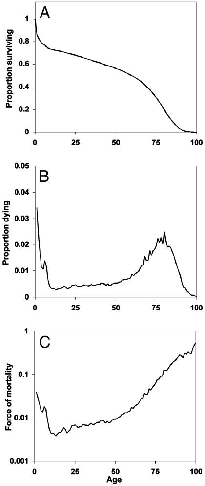
Fig. 1 plots l(a), d(a), and μ(a) for the cohort of females born in Sweden in 1850. The survival function declines to zero at around age 100 yr. The density function is broadly bimodal with peaks at age 0 and ≈80 yr. The force of mortality exhibits a U-shaped pattern with a minimum at about age 10. Note the use of the log scale to accommodate the large differences in magnitude at different ages. These patterns are broadly typical, although levels of mortality vary widely between populations and over time.

Fig. 1.

Mortality experience of the cohort of Swedish females born in 1850, as summarized by the survival function, l(a)(A), the death density function d(a) (B), and the force of mortality function μ(a) (C).

Mean lifetime for a birth cohort, M, may be calculated from l(a) as

[2a]

from d(a) as

[2b]

or from μ(a) as

[2c]

These formulas give identical results. For the 1850 cohort of Swedish females, for example, we calculate M = 48.1 yr from each.

Period Mean Lifetime. Let

[3a]

[3b]

[3c]

where the subscripts at right indicate time of birth. Thus l(a, t) denotes the proportion of persons born at time t - a who are surviving at time t; d(a, t) denotes the density of deaths for this cohort at age a and time t; and μ(a, t) denotes the corresponding force of mortality. Note that l(a, t) and d(a, t) differ from the survival and density functions for synthetic cohorts obtained from conventional period life tables, and that their calculation requires data on either past births and migrations or on past deaths.

We refer to l(a, t) as the standardized population age distribution at time t and to d(a, t) as the standardized age distribution of deaths at time t. The standardized population age distribution and age distribution of deaths are the same as their unstandardized counterparts in any population that experiences constant numbers of births over time.

By analogy with Eq. 2, mean lifetime at time t may be calculated as

[4a]

[4b]

[4c]

Each of these formulas has been used in demography to calculate period mean age for some demographic event. Mean age at first marriage is often calculated as a variant of M₁(t) that allows for persons not marrying. This is the singulate mean age at marriage introduced by Hajnal (2), with l(a, t) taken as the proportion of single persons at age a at time t (see, for example, ref. 3). Mean age at childbearing is generally calculated as M₂(t), with age-specific or age-order-specific birth rates substituted for d(a, t) (see, for example, ref. 4). Life expectancy at birth, denoted e₀(t), is conventionally calculated as M₃(t).

We refer to M₂(t) as the standardized mean age at death. The unstandardized mean age at death is unacceptable as a measure of mean lifetime, because it may be heavily distorted by the population age distribution. This objection does not apply to the standardized mean age at death, which might be a widely used measure of period mean lifetime if it were more easily calculated.

If l(a, t) is constant with respect to t, the three means defined by Eq. 4 are identical. When length of life changes, the three means diverge. The following sections develop relationships among them.

Results

Relation Between M₁ and M₂. To establish a simple relationship between M₁(t) and M₂(t), let

[5a,b]

The age schedules d_s(a, t) and μ_s(a, t) are inherent in the standardized population age distribution at time t. They may be interpreted as the age distribution of deaths and the force of mortality function in the stationary population whose age distribution is given by l(a, t), with l(0, t) = 1 for all t. This interpretation is, of course, valid only if the mortality history of the population is such that l(a, t) is a nonincreasing function of a (dl(a, t)/da ≤ 0).

Assume now that for t in the time interval [0, Δ], there exists a function p(t) independent of age, such that

[6a]

[6b]

and that the function p(t) is a real valued integrable function bounded below by 0. We refer to this as the proportionality assumption.

The proportionality assumption implies that the age schedules of μ(a, t) and d(a, t) are the same in shape (but not necessarily level) as the age schedules of μ_s(a, t) and d_s(a, t). As will be shown below, this assumption provides a good approximation for patterns of adult mortality in contemporary countries with high life expectancy.

From Eqs. 4a and 5a,

[7a]

and from Eqs. 4b and 6b,

[7b]

On cancellation of the proportionality factor p(t), Eq. 7b becomes Eq. 7a, thus proving that M₁(t) = M₂(t).

Other Implications of the Proportionality Assumption. It is shown in Appendix 1 that if the proportionality assumption holds, then

[8a]

Substituting this in Eq. 6 and noting that M₁(t) = M₂(t) yields

[8b]

[8c]

This shows that μ(a, t) and d(a, t) are functions of the rate of change in the standardized mean age at death M₂(t), because μ_s(a, t) and d_s(a, t) are determined by mortality conditions up to time t. When this mean age is rising, μ(a, t) < μ_s(a, t) and d(a, t) < d_s(a, t), but when it is declining, μ(a, t) > μ_s(a, t) and d(a, t) > d_s(a, t).

As shown in Appendix 2, the proportionality assumption also implies that the age schedule l(a, t) shifts uniformly to older (younger) ages as the mean age at death rises (falls). Uniform shifting between time 0 and time T means that there is a function F(t) = M₁(t) - M₁(0), giving the magnitude of the shift between time 0 and time t, such that, for all 0 ≤ t ≤ T,

[9]

and l(a, t) = 1 for a < F(t). Downward as well as upward shifts are possible, provided that l(a, t) = 1 for a less than some number > 0.

It follows from Eq. 5 that uniform shifts in l(a, t) imply uniform shifts in μ_s(a, t) and d_s(a, t) with the same shift function F(t), with μ_s(a, t) = d_s(a, t) = 0 when l(a, t) = 1. The proportionality assumption is therefore equivalent to the shifting assumption made by Bongaarts and Feeney (5).

Changes over time in the schedules μ(a, t) and d(a, t) are of two types. First, as the mean age at death rises or falls, μ(a, t) and d(a, t) shift to higher or lower ages with l(a, t), μ_s(a, t), and d_s(a, t). Second, μ(a, t) and d(a, t) are deflated or inflated relative to μ_s(a, t) and d_s(a, t) by the proportionality factor p(t).

Mortality Change in France, Sweden, and the U.S. We will now show that observed mortality patterns conform closely to the proportionality assumption (Eq. 6) if child and young adult mortality is ignored. All quantities in this section, in Figs. 2,3,4,5,6, and in Table 1 are calculated from observed values of μ(a, t) for ages >30, but μ(a, t) is set to zero for ages <30 years for all t. Our estimates of life expectancy at birth are therefore equal to 30 plus the life expectancy at age 30. For populations with high life expectancy, nearly all deaths (97–98%) occur at ages >30 yr, and actual life expectancy at birth is therefore close to 30 plus the life expectancy at age 30.

Fig. 2.

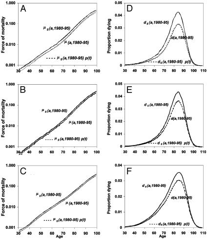
Average force of mortality for 1980–1995, observed as μ(a, t), estimated from l(a, t) as μ_s(a, t), and estimated as the product μ_s(a,1980–1995)p(t) for France (A), Sweden (B), and the U.S. (C). Also shown is the average death density function for 1980–1995, observed as d(a, t), estimated from l(a, t) as d_s(a, t), and estimated as the product d_s(a,1980–1995)p(t) for France (D), Sweden (E), and the U.S. (F).

Fig. 3.

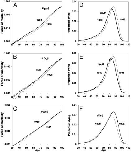
Observed period force of mortality μ(a, t) in 1980 and 1995 for France (A), Sweden (B), and the U.S. (C). Also shown is the observed period death density function d(a, t) in 1980 and 1995 for France (D), Sweden (E), and the U.S. (F).

Fig. 4.

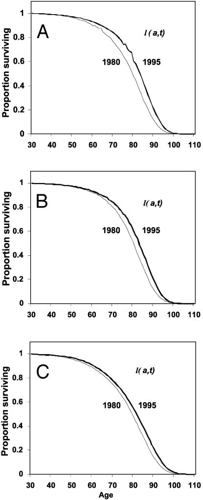
Observed period survival function l(a, t) in 1980 and 1995 for France (A), Sweden (B), and the U.S. (C).

Fig. 5.

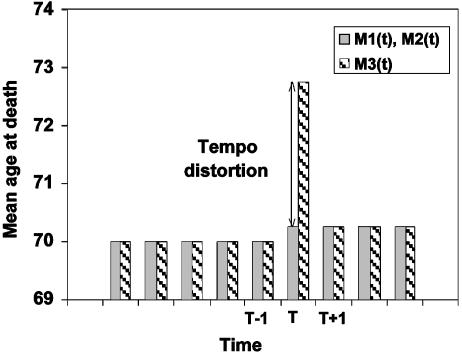
Hypothetical illustration of effect of increase in mean age at death by 0.25 yr (from 70.0 to 70.25) during year T on conventional life expectancy. Before and after T, M₁(t) = M₂(t) = M₃(t). During T, a tempo distortion of -25% in the number of deaths results in an upward distortion of ≈2.5 yr in M₃(t).

Fig. 6.

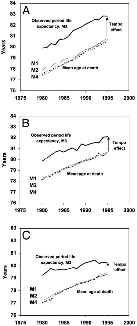
Trends from 1980 to 1995 for alternative estimates of mean age at death M₁, M₂, M₃, and M₄ for France (A), Sweden (B), and the U.S. (C). The difference M₃ - M₄ equals the tempo effect.

Table 1. Alternative estimates of the period mean age at death (assuming no mortality under age 30).

	Mean age at death, females, 1980—1995
	M1(t)	M2(t)	M3(t) (= e0(t))	M4(t)	Tempo effect M3(t)-M4(t)
France	79.0	79.2	81.4	79.0	2.4
Sweden	79.5	79.5	81.1	79.4	1.6
U.S.	78.3	78.3	79.9	78.3	1.6

Source: Death rates from University of California, Berkeley Mortality Data Base, available at www.demog.berkeley.edu/wilmoth/mortality.

Fig. 2 A–C shows the age schedules, μ(a, t), μ_s(a, t), and p(t)μ_s(a, t), all calculated as averages of annual values for 1980–1995, for France, Sweden, and the U.S. Fig. 2 D–F shows the age schedules d(a, t), d_s(a, t), and p(t)d_s(a, t) calculated in the same way with p(t) estimated with Eq. 8a. The near coincidence of μ(a, t) and p(t)μ_s(a, t) and of d(a, t) and p(t)d_s(a, t) shows that the proportionality assumption is a good approximation for all three countries. Note that the logarithmic scale used in Fig. 2 A–C means that perfect proportionality corresponds to constant differences between the plotted values of μ(a, t) and μ_s(a, t).

Fig. 3 A–C shows μ(a, t) for 1980 and 1995 for the same three countries. Fig. 3 D–F shows corresponding values for d(a, t). The pattern of change in these schedules is consistent with the pattern of shifting and inflation/deflation noted above.

Fig. 4 plots the age schedule l(a, t) for 1980 and 1995 for the three countries. The shape of l(a, t) changes very little, but there is a shift to higher ages as life expectancy rises. The magnitude of the shift was 3.4 yr for France, 2.4 yr for Sweden, and 2.1 yr for the U.S.

The first three columns of Table 1 present averages of annual estimates of M₁(t), M₂(t), and M₃(t) for the years 1980–1995. The values for M₁(t) and M₂(t) are nearly identical, as expected, but the M₃(t) values are substantially higher. The reason for the higher value of M₃(t) is discussed below.

Tempo Effects in Demographic Analysis. Tempo effects were first discovered and analyzed in the study of fertility. If women shift the ages at which they bear children upward without changing their completed fertility, annual numbers of births will be less than they would have been, because the same number of births will be spread out over a longer time period. Similarly, if women begin to have children at younger ages, annual numbers of births will be larger than they would have been, because the same number of births occurs over a shorter time period. These changes in annual number of births induced by changes in the timing of childbearing are tempo effects.

Fertility tempo effects have been extensively documented. The postwar “baby boom” in the U.S., for example, was due in part to a decline in the mean age at childbearing during the late 1940s and the 1950s (6–9).

Tempo effects complicate the study of levels and trends of fertility, because they produce changes in period fertility rates that depend on the rate at which the mean age at childbearing changes, independently of changes in completed fertility of cohorts. Ryder (10) introduced the term “timing distortion” to refer to tempo effects, because they are undesirable in most analyses of fertility levels and trends.

Tempo effects influence demographic processes other than fertility. A tempo effect can be defined in general as an inflation or deflation of the period incidence of a demographic event (births, marriages, and deaths) resulting from a rise or fall in the mean age at which the event occurs.

Tempo Effects in Mortality. A simple example will demonstrate how mortality tempo effects operate. Consider a stationary population with a life expectancy at birth of 70 yr. Suppose the exact age of death of each individual is predetermined until the invention of a “life extension” pill that adds 3 mo to the life of any person who consumes it.

If everyone in the population takes this pill on January 1 of year T, there will be no deaths during the first 3 mo of the year. The number of deaths in year T will fall by 25%, and the mean age at death will rise from 70 to 70.25 yr. Because the pill's effect is the same at all ages, the level of the force of mortality function is also reduced by 25%, and the age to which each value of the function is attached increases by 0.25 yr. This fall in values of the force of mortality function, together with the shift to older ages, causes life expectancy at birth as conventionally calculated to rise to ≈73 yr for year T.

In the next year, the number of deaths and the force of mortality function rise to the level observed before year T, but with values shifted forward to older ages by 0.25 yr. Life expectancy at birth as conventionally calculated, having risen from 70 yr prior to year T to ≈73 yr during year T, falls back to 70.25 yr (Fig. 5). We contend that this temporary rise in life expectancy at birth as conventionally calculated is a tempo distortion, because it is at variance with the known trend in the mean length of life. Distortion of this kind occurs whenever the standardized mean age at death changes.

Removing Tempo Effects. The tempo effect deflates (inflates) d(a, t) and μ(a, t) when the standardized mean age at death rises (falls). Formulas 8b,c show this deflation or inflation is estimated by the multiplicative factor 1 - ∂M₂(t)/∂t when the proportionality assumption holds. The tempo effect may therefore be removed by dividing d(a, t) and μ(a, t) by 1 - ∂M₂(t)/∂t. Because M₁(t) = M₂(t), division by 1 - ∂M₁(t)/∂t gives the same result. The latter approach is preferred, because it gives more stable results when applied to observed mortality rates. We define

[10a]

[10b]

and refer to the expressions on the left as the tempo-adjusted death density and force of mortality. It follows from Eq. 8 that μ^*(a, t) = μ_s(a, t) and d^*(a, t) = d_s(a, t) when the proportionality assumption holds.

To calculate life expectancy at birth corrected for the tempo effect, the defining formula 4c is used with μ^*(a, t) substituted for μ(a, t), giving

[11]

where M₄(t) denotes life expectancy at birth without the tempo effect. Removing the tempo effect from M₃(t) gives the same result as M₁(t) or M₂(t). The undistorted life expectancy at birth can be estimated as M₁(t), M₂(t), or M₄(t).

Table 1 shows average annual values of M₄(t) as well as M₁(t), M₂(t), and M₃(t) for females in France, Sweden, and the U.S. for the period 1980–1995. The corresponding annual trends are plotted in Fig. 6. These results confirm that M₁(t), M₂(t), and M₄(t) are nearly identical, but M₃(t), the life expectancy at birth calculated by conventional life table methods, is substantially higher than the other three means. The tempo effect, M₃(t) minus M₄(t), averages 2.4 yr for France and 1.6 yr for Sweden and the U.S.

This analysis of tempo effects is based on trends in adult mortality only. We ignore any tempo effects in mortality under age 30, because they are probably small and difficult to quantify. In the absence of tempo effects under age 30, the tempo effect in life expectancy at birth is only 2% or 3% smaller than the tempo effect above age 30 measured here. This is because the probability of survival from birth to age 30 is typically 0.98–0.97 in contemporary societies with high life expectancy.

Conclusion

Life expectancy at birth as conventionally calculated is distorted whenever it is changing. We have provided formulas to adjust for this distortion. The formulas are applicable to populations with high life expectancy. The adjustments for France, Sweden, and the U.S. in recent decades reduce conventionally calculated life expectancy at birth by 1.6 to 2.4 yr. These results confirm and extend those given in Bongaarts and Feeney (5).

The essential argument is as follows. Empirical observation indicates that the proportionality assumption is closely approximated when life expectancy at birth is high and child and young adult mortality are ignored. When the proportionality assumption holds, increases (decreases) in length of life are realized by a uniform translation of the standardized population age distribution and the force of mortality function inherent in this age distribution to higher (lower) ages. Neither the shape nor the level of the standardized age distribution or the inherent force of mortality function changes; only their location on the age scale changes.

The force of mortality function is likewise translated to higher (or lower) ages without any change in shape, but its level changes with the rate of change in the standardized mean age at death, as shown by Eq. 8b. When the standardized mean age at death rises (falls), the force of mortality function falls and shifts to the right (rises and shifts to the left). This fall (rise) in the force of mortality represents the tempo effect and produces an undesirable rise (fall) in life expectancy at birth as conventionally calculated. In our hypothetical example (Fig. 5), increasing the standardized mean age at death from 70 to 70.25 yr over 1 yr results in a temporary decline of 25% in the force of mortality function and a temporary rise of nearly 3 yr in conventionally calculated life expectancy at birth. The tempo effect in life expectancy in this case is ≈10 times the net change in mean lifetime.

In interpreting these findings, it is important to distinguish between current observed death rates and current mortality conditions (11). We do not question the conventional life table calculation of period life expectancy from observed age-specific death rates. We argue rather that tempo effects distort both the observed death rates and the corresponding life expectancy, so that their values give a misleading indication of current mortality conditions.

Our empirical focus has been on human survival, but life table methods are widely applied to survival data of all kinds. Examples include age at marriage (the interval between birth and marriage), birth interval analysis (intervals between successive births), length of schooling (interval between entering and leaving school), and postoperative survival (interval between operation and death). It is therefore likely that tempo effects are pertinent to many other kinds of statistical survival analyses.

Appendix 1

We have to prove that the proportionality assumption (Eq. 6) implies Eq. 8a of the text. Bennett and Horiuchi (12), Preston and Coale (13), and Arthur and Vaupel (14) show that

[A1]

where

[A2]

is the age-specific growth rate for age a at time t for the population whose age distribution at time is t given by l(a, t). Note that Eq. A1 may be written as

[A3]

which is an equation used in modeling cell population dynamics (15–18). Equating the expressions for μ(a, t) given by the proportionality assumption (Eq. 6a) and Eq. A1 and rearranging terms gives

[A4]

Substitution of Eqs. A2 and 5b in Eq. A4 yields

[A5]

From the definition (Eq. 4a) of M₁(t), then,

[A6]

Because the last integral on the right equals one, we have established formula 8a of the text.

Integrating the density function d(a, t) over age results in a period mortality measure that may be called the total mortality rate TMR(t). (This measure is equivalent to the total fertility rate widely used in the analysis of fertility levels and trends.)

[A7]

Substitution of Eq. 8a gives

[A8]

Appendix 2

We have to prove that the proportionality assumption implies uniformly shifting age distributions, i.e., Eq. 9, provided there is no mortality at younger ages. The first step is to find a characterization of uniformly shifting age distributions that applies to a point in time. The directional derivative provides such a characterization. The directional derivative of the function l(a, t) at the point (a, t) in the direction (b, u) is the rate of change at time t of the function l(a + bt, t + ut), which may be expressed as

[A9]

Now let f(a, t) be such that the directional derivative of l(a, t) at the point (a, t) in the direction (f(a, t),1) equals zero. Uniform translation corresponds to the condition that f(a, t) be constant with respect to age, f(a, t) ≡ f(t) for all t, and therefore to the condition

[A10]

If this identity holds, the directional derivative of l(a, t) at the point (a, t) in the direction (f(t), 1) is zero.

If the proportionality assumption holds, text formula 8b holds (as just shown in Appendix 1), and this together with Eq. A1 implies, equating the expressions for μ(a, t) and rearranging terms,

[A11]

Multiplying both sides by -l(a, t) gives

[A12]

which shows that the directional derivative of l(a, t) at (a, t) in the direction (f(t), t) equals 0 for all ages a, with f(t) = ∂M₁(t)/∂t.

To show that this implies uniform shifting of the age distribution, it is necessary only to note that f(t) is the rate of change of the contour line in the age-time plane defined by the points (x + t, t) for which l (x + t, t) = l (a, 0). The function F(t) of the uniform shifting formula (Eq. 9) therefore equals the integral of f(·) from 0 to t.

References

- 1.Preston, S. H., Heuveline, P. & Guillot, M. (2001) Demography: Measuring and Modeling Population Processes (Blackwell, Malden, MA).
- 2.Hajnal, J. (1953) Popul. Studies 7, 111-136. [Google Scholar]
- 3.United Nations (1990) Patterns of First Marriage (United Nations, New York).
- 4.Council of Europe (2001) Recent Demographic Developments in Europe 2001 (Council of Europe Publishing, Strasbourg, France).
- 5.Bongaarts, J. & Feeney, G. (2002) Popul. Dev. Rev. 28, 13-29. [Google Scholar]
- 6.Hajnal, J. (1947) Popul. Studies 1, 137-164. [Google Scholar]
- 7.Ryder, N. B. (1964) Demography 1, 74-82. [Google Scholar]
- 8.Ryder, N. B. (1980) in Demographic Patterns in Developed Societies, ed. R. W. Hiorns (Taylor & Francis, London), pp. 15-54.
- 9.Bongaarts, J. & Feeney, G. (1998) Popul. Dev. Rev. 24, 271-291. [Google Scholar]
- 10.Ryder, N. B. (1956) Milbank Mem. Fund Q. 34, 5-21. [PubMed] [Google Scholar]
- 11.Vaupel, J. W. (2002) Demog. Res. 7, 365-377. [Google Scholar]
- 12.Bennett, N. & Horiuchi, S. (1981) Popul. Index 47, 207-221. [Google Scholar]
- 13.Preston, S. H. & Coale, A. J. (1982) Popul. Index 48, 217-259. [PubMed] [Google Scholar]
- 14.Arthur, W. B. & Vaupel, J. W. (1984) Popul. Index 50, 214-226. [PubMed] [Google Scholar]
- 15.McKendrick, A. G. (1926) Proc. Edinburgh Math. Soc. 40, 98-130. [Google Scholar]
- 16.Von Foerster, H. (1959) in The Kinetics of Cellular Proliferation, ed. Stohlman, F. (Grune and Stratton, New York), pp. 382-407.
- 17.Trucco, E. (1965) Bull. Math. Biophys. 27, 285-304. [DOI] [PubMed] [Google Scholar]
- 18.Trucco, E. (1965) Bull. Math. Biophys. 27, 449-470. [DOI] [PubMed] [Google Scholar]