

Abstract
Interaural time difference (ITD) plays a central role in many auditory functions, most importantly in sound localization. The classic model for how ITD is computed was put forth by Jeffress (1948). One of the predictions of the Jeffress model is that the neurons that compute ITD should behave as cross-correlators. Whereas cross-correlation-like properties of the ITD-computing neurons have been reported, attempts to show that the shape of the ITD response function is determined by the spectral tuning of the neuron, a core prediction of cross-correlation, have been unsuccessful. Using reverse correlation analysis, we demonstrate in the barn owl that the relationship between the spectral tuning and the ITD response of the ITD-computing neurons is that predicted by cross-correlation. Moreover, we show that a model of coincidence detector responses derived from responses to binaurally uncorrelated noise is consistent with binaural interaction based on cross-correlation. These results are thus consistent with one of the key tenets of the Jeffress model. Our work sets forth both the methodology to answer whether cross-correlation describes coincidence detector responses and a demonstration that in the barn owl, the result is that expected by theory.
Keywords: barn owl, interaural time difference, cross-correlation, coincidence detection, sound localization, nucleus laminaris
Introduction
Both mammals and birds use interaural time difference (ITD) as a cue to determine the horizontal position of a sound source in space (Moiseff, 1989; Heffner and Heffner, 1992). The basic model to explain the computation of ITD uses a combination of coincidence detection and delay lines to produce neurons that fire maximally when the differences in arrival time of the sound at each ear and the neural conduction delays cancel each other exactly (Jeffress, 1948). Consistent with this, the axons that project to nucleus laminaris (NL) of the barn owl act as delay lines converging on neurons that act as coincidence detectors (Carr and Konishi, 1988, 1990). Even in mammals, where the exact method of encoding ITDs is under question (McAlpine et al., 2001; Joris and Yin, 2007), the neurons of the medial superior olive (MSO), the homolog to NL, behave as coincidence detectors (Goldberg and Brown, 1969; Yin and Chan, 1990). The coincidence detection model has been argued to be a special case of a more general cross-correlation algorithm (Licklider, 1959) that expresses the degree of similarity between two time-dependent signals as a function of relative delay. Experiments have verified that the neurons of NL and MSO do show cross-correlation-like behavior (Yin et al., 1987; Carr and Konishi, 1990; Yin and Chan, 1990). However, attempts to show that the shape of the ITD response function is exactly determined by the spectral tuning of the neuron, a core prediction of cross-correlation, have been unsuccessful (Yin et al., 1987; Batra and Yin, 2004). This becomes an important issue in light of recent results arguing that ITD selectivity is shaped by inhibition (Brand et al., 2002; Seidl and Grothe, 2005), which would represent a major revision to the basic Jeffress model. Therefore, the extent to which cross-correlation is a description of the behavior of NL and MSO neurons remains an open question, and with it, the completeness of the current coincidence detection model.
If NL neurons do behave as cross-correlators, then the cross-correlation theorem predicts a precise relationship between power spectra of the ITD response curve and the effective stimulus, in which the effective stimulus is the portion of the stimulus that passes the various cochlear and neural filters and succeeds in stimulating the neuron. Specifically, the cross-correlation theorem predicts equality of the power spectrum of the ITD response curve and the square of the power spectrum of the effective stimulus (see supplemental material, available at www.jneurosci.org). Additionally, we should be able to predict NL responses from a cross-correlation of the effective monaural inputs. In this study, we test the prediction of the cross-correlation theorem by comparing the power spectrum of the ITD response curve and the square of the power spectrum of the spike-triggered average (STA). We also use binaurally uncorrelated noise to estimate the effective monaural inputs and develop a model of NL spiking responses to test whether cross-correlation describes binaural interaction in NL neurons.
Materials and Methods
Surgery.
Owls were anesthetized by intramuscular injection of ketamine hydrochloride (20 mg/kg Ketaject; Phoenix Pharmaceuticals) and xylazine (2 mg/kg, Xyla-Ject; Phoenix Pharmaceuticals). An adequate level of anesthesia was maintained by additional injections of both when needed. All experiments were performed under anesthesia. During the first recording session, ear bars and a beak holder were used to position the owl's head with the beak rotated 70° in the sagittal plane. A head plate was implanted by removing the top layer of the skull and fixing the plate with dental cement. A stainless steel reference post was implanted posterior to the head plate and similarly fixed with dental cement. Once the head plate was implanted, the ear bars and beak holder were removed, and the head plate was used to hold the head in position from that point forward and in all following recording sessions. A craniotomy was made over the recording site. The craniotomy was packed with gelfoam and sealed with dental cement, and the scalp was sutured at the end of the session. After the surgery, analgesics (Ketoprofen, 10 mg/kg Ketofen; Merial) were administered. The protocol for this study followed the National Institutes of Health Guide for the Care and Use of Laboratory Animals and was approved by the Animal Care and Use Committee of the California Institute of Technology and the Animal Institute Committee of the Albert Einstein College of Medicine.
Electrophysiology.
We positioned the recording electrodes by known stereotaxic coordinates and by the response properties of the units, obtained using white noise and tones of manually set ITD and frequency as search stimuli. NL is easily identified by the large field potentials (called neurophonics) that vary in amplitude with ITD. We isolated and maintained NL single neurons by a “loose patch” method (Peña et al., 1996, 2001) in which the electrode served as a suction electrode, allowing us to obtain stable recordings lasting for >1 h. The loose patch recording technique was developed to overcome the traditional difficulty in obtaining stable and well isolated recordings of coincidence detector neurons in NL and in its mammalian equivalent, the MSO. During the recordings, the neurons showed a high degree of phase locking and stable tuning to ITD. Also, we have previously shown that NL neurons recorded by loose patch have tuning to ITD that is tolerant to a broad range of sound intensity (Peña et al., 1996) and precisely matches the values expected by conduction delays of afferent fibers published in previous studies (Carr and Konishi, 1990; Peña et al., 2001).
Neural signals were serially amplified by an Axoclamp-2A (Molecular Devices) and a custom-made AC amplifier (μA-200; Beckmann Electronics Shop, California Institute of Technology, Pasadena, CA). A spike discriminator (SD1; Tucker-Davis Technologies) converted neural impulses into transistor–transistor logic pulses for an event timer (ET1; Tucker-Davis Technologies), which recorded the timing of the pulses. A computer was used for stimulus synthesis and on-line data analysis.
Acoustic stimulation.
An earphone assembly consisting of a Knowles 1914 receiver, a Knowles 1743 damping device, and a Knowles 1939 microphone delivered sound stimuli. These components are encased in an aluminum cylinder that fits into the owl's ear canal. The gaps between the cylinder and the ear canal were filled with silicon impression material (Gold Velvet II; Earmold & Research Laboratory). At the beginning of each experimental session, the earphone assemblies were automatically calibrated. The computer was programmed to equalize sound pressure level and phase for all frequencies within the frequency range relevant to the experiment.
Tonal and broadband stimuli 100 ms in duration with 5 ms rise/fall times were presented once per second. We used PA4 digital attenuators (Tucker-Davis Technologies) to vary stimulus sound levels.
Data collection.
Long-range ITD curves were obtained by scanning ITD in 10–30 μs steps from ±1500 to ±2500 μs with broadband signals (1–12,000 kHz) each repeated 5–10 times. For the purposes of testing the cross-correlation hypothesis, reverse correlation data (see below) can theoretically be obtained at any ITD. To maximize firing rate, and hence minimize the time required to collect data, we chose an ITD at the peak of the rate-ITD function. In the cat MSO, the characteristic delay (CD) (Rose et al., 1966) is known to fall at or near peaks of the rate-ITD function (Yin and Chan, 1990), and the lack of phase-locked inhibition in the avian NL (Yang et al., 1999) suggests the same should be true in the owl. Therefore, for the sake of consistency between neurons, we used tonal ITD-rate functions to estimate a frequency-independent ITD, as described by Peña et al. (2001). This method will reliably produce the CD when the CD falls at a peak (Yin and Kuwada, 1983), and we refer to this ITD as the estimated CD.
Isointensity frequency tuning curves (FTCs) were obtained for sound levels 20–30 dB above threshold with randomized sequences of stimulus frequencies in steps of 100 Hz at the CD of the neuron.
Data for reverse correlation were obtained by presenting 100 ms band-limited Gaussian white noise (0.5–12,000 kHz) signals at the estimated CD of each neuron, randomly interleaved with stimuli at a different ITD; stimuli were presented with an interstimulus interval of 500 ms, and we attempted to collect between 400 and 800 trials for each ITD condition. For each stimulus presentation, the signal was synthesized de novo to avoid correlation artifacts. The sound intensities used for isointensity FTCs, long-range ITD curves, and reverse correlation were the same. To control for the possibility that the spectrum of the STA depends on the ITD of the stimulus used in the reverse correlation, we also collected reverse correlation data using ITDs other than the estimated CD, covering both other peaks of the rate-ITD function and values intermediate between peaks and troughs.
Analysis.
FTCs were characterized by their width (W50). W50 is the range of frequencies over which the discharge rate of the cell was equal to 50% of the difference between the maximal discharge rate and the spontaneous level.
The window of the reverse correlation (i.e., the amount of stimulus preceding each spike that was considered in the analysis) was 15 ms; visual examination indicated that none of the neurons in our population had a response function with a temporal extent that exceeded that limit. To ensure that segments of the interstimulus interval and the rise period of the stimulus were not included in the reverse correlation analysis (or, in other words, to guarantee that the reverse correlation was done on a signal with stationary statistics), spikes that occurred in the 20 ms immediately after stimulus onset were excluded; this exclusion was also sufficient to guarantee that the onset transient was excluded and that the neuron had reached a stable firing rate, and we encountered no neurons that had onset-only responses. After this exclusion, a large number of spikes remained for consideration (average number of spikes used in the reverse correlation analysis per neuron was 4158 ± 1818).
We tested the prediction of the cross-correlation theorem by comparing the power spectral density (PSD) of the ITD response curve and the square of the PSD of the STA (see supplemental material, available at www.jneurosci.org). The power was measured on a decibel scale, and therefore we compared the widths of the PSDs using the 10 dB bandwidth of the ITD response curve and the 5 dB bandwidth of the STA, to take into account the squaring of the latter predicted by the cross-correlation theorem. We compared the locations of the peaks in the PSDs using the center frequencies of the 10 dB bandwidth for the ITD response and the 5 dB bandwidth for the STA. PSD was estimated with the MATLAB implementation of Thomson's multitaper method. The reverse correlation was done with a 15 ms window at a sampling rate of 48,077 Hz, whereas the ITD curve was sampled with 30 μs resolution over a range of no more than 4.8 ms. To remove the effects caused by the differences in sampling rate and temporal extent, the reverse correlation data were down-sampled to the sampling rate of the ITD curve, and then a time window matching that of the ITD curve was chosen about the maximum absolute value of the STA.
Model of coincidence detector responses.
We used a linear–nonlinear Poisson model to describe the responses of coincidence detector neurons in NL (Chichilnisky, 2001). The instantaneous spiking probability conditioned on the left and right auditory input signals is given by the following:
where sL(t) and sR(t) are monaural input signals, sL and SR denote the monaural inputs at all time points up to and including t kL(t) and kR(t) are monaural filters, the asterisk represents convolution, and f is a static input–output function that transforms the pair of filtered input signals into the instantaneous spiking probability. Spikes are produced using an inhomogeneous Poisson process.
We estimated the monaural filters and the input–output nonlinearity for six neurons using responses to binaurally uncorrelated stimuli. The monaural filters kL(t) and kR(t) were estimated by the STAs of the left and right input signals, respectively. We estimated the input–output nonlinearity as f(s1, s2) = P(spike | s1, s2), where the input signals s1(t) = kL * sL(t) and s2(t) = kR * sR(t) are computed by convolving the left and right stimuli with their associated monaural filters. Using Bayes' rule, we write the input–output nonlinearity f(s1, s2) = P(spike | s1, s2) as f(s1, s2) = αP(s1, s2 | spike)/P(S1, S2). We estimated the prior P(s1, s2) by a Gaussian kernel density estimate, using values of s1 and s2 computed from an ensemble of randomly selected stimulus segments. Similarly, we estimated the likelihood P(s1, s2 | spike) by a Gaussian kernel density estimate using values of s1 and s2 computed from the ensemble of spike-triggered stimuli. Kernel widths were adjusted for each neuron so that the estimated spiking probability appeared smooth. We found that the NL data are consistent with a linear-quadratic model (see Results). Therefore, model simulations were performed where the instantaneous spiking probability is given by a quadratic function:
 |
where a, b, and c are constants that are selected from finite ranges to give the minimum mean square difference between the model ITD curve and the experimentally measured ITD curve.
Results
We used a sample of 77 NL neurons recorded in 12 adult barn owls (Tyto alba) of both sexes, bred in captivity. Seventeen of these units were used in the reverse correlation analysis.
The effective input to NL neurons
We used reverse correlation to determine the stimulus features to which NL neurons are sensitive (de Boer and de Jongh, 1978). The loose-patch technique (see Materials and Methods) (Peña et al., 1996, 2001) allowed us to obtain the quality and stability of recording (Fig. 1a) necessary to apply reverse correlation analysis (de Boer and de Jongh, 1978; Christianson and Peña, 2007). The ITD-dependent response of NL neurons is different in the case of a tone versus a broadband noise signal (Fig. 1b). In particular, the decaying amplitude of the ITD response curve for broadband noise indicates that the neuron is being driven by a range of frequencies; we refer to this range and the driving power of the frequencies within that range as the effective input. We estimated the PSD of the effective input by computing the PSD of the STA response to broadband noise (Fig. 2a), because the STA is an estimate of the linear impulse response of the neuron and therefore the best linear filter that approximates the spectrotemporal tuning of the neuron.
Figure 1.

ITD response curves. a, Laminaris neuron recorded with loose patch. When the firing rate is plotted as a function of ITD in response to broadband stimuli and the range of ITDs is limited to those that might be encountered under normal listening conditions, the resulting curve can show multiple peaks of similar amplitude, similar to a cosine. Two example traces show the response to favorable and unfavorable ITDs indicated by the arrows. The poststimulus time histogram (PSTH) and interspike interval histogram (ISIH) are shown on the right. b, Example of a long-range ITD curve for another laminaris neuron. When the range of ITDs presented is expanded, a more complex structure becomes evident. Whereas the response is periodic for tonal stimulation (thin line), the amplitude of the peaks decays in response to a broadband sound as a result of the bandpass filtering of signals in the cochlea (bold line). For the physiological range (Phys. Range; inset), the responses to tones and broadband signals are practically indistinguishable.
Figure 2.
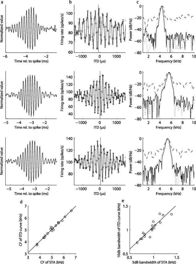
STA and ITD tuning. Relationship between power spectra of the ITD response and the STA. a, b, All neurons had a coherent STA response to noise (a) and ITD response curve (b). c, The doubled PSD of the STA (solid line) corresponds to the power spectra of the ITD curve (dashed line). By adjusting the sampling resolution, the doubled PSD of the STA (dashed line) better matches the PSD of the ITD curve. The top panels show the STA (a), ITD response curve (b), and the PSD (c) for three laminaris neurons. The vertical line in b indicates the estimated CD of the neuron (see Materials and Methods). rel., Relative. d, The center frequency (CF) of the PSD of the STA is highly correlated with the CF of the PSD of the ITD curve (n = 17). The solid line is the regression line. The 5 dB bandwidth of the PSD of the STA, with sampling rate compensation, is shown plotted against the 10 dB bandwidth of the ITD curve in e (n = 17). The solid line is the regression line.
Spectral tuning of input and output
We tested the prediction of the cross-correlation theorem that the power spectrum of the ITD response curve is equal to the square of the power spectrum of the effective stimulus. The center frequencies of the PSD of the ITD response curve and the square of the PSD of the STA were highly correlated (regression, 0.99x + 115 Hz; n = 17; r2 = 0.98) (Fig. 2d). We compared bandwidths using the 10 dB bandwidth of the ITD response curve and the 5 dB bandwidth of the STA (Fig. 2a,b) (see Materials and Methods). The correlation was good, with a linear regression near unity, as predicted by theory (regression, 0.98x + 320 Hz; n = 17; r2 = 0.84). A large offset between the two is explained by the fact that the ITD response curve was sampled at much lower resolution than the reverse correlation data. When the reverse correlation data were down-sampled to account for this (Fig. 2c), the offset dropped dramatically (regression, 0.94x + 131 Hz; n = 17; r2 = 0.86) (Fig. 2e).
To test whether errors in our estimation of the CD could bias the results, we obtained STAs at different ITDs for a subset of these neurons (n = 15). There was no significant difference in center frequencies (Fig. 3a) and bandwidths (Fig. 3b) between STAs measured using different ITDs (sign test not significant; p > 0.8). Neither did we find a dependence between the difference of bandwidths and the phase difference between the ITDs (linear regression not significantly different than zero; p > 0.3; r2 = 0.06). This is consistent with previous results showing that the spectrotemporal tuning in the owl's inferior colliculus does not appear to depend on sound direction (Keller and Takahashi, 2000).
Figure 3.

Power spectra of STAs at different ITDs. We obtained STAs at different ITDs for a subset of the neurons (n = 15). The center frequencies (a) and 5 dB bandwidths (b) of PSDs of STAs collected using the estimated CD and ITDs off the estimated CD are correlated. The solid lines are identity lines. CF, Center frequency.
We also compared the PSD of ITD curves of 77 neurons with the isointensity FTC, which is a plot of mean spike rate as a function of frequency (Fig. 4a). Correlation between bandwidths was observed as in the comparison of the PSD of the ITD curve and the PSD of the STA, although weaker, and squaring the FTC, as per the cross-correlation theorem (see supplemental material, available at www.jneurosci.org), did not improve the correlation (Fig. 4b). Because the FTC is known to be a poor estimate of the effective spectral response of the neuron (Spezio and Takahashi, 2003), this lower degree of correlation is to be expected.
Figure 4.

Comparison of power spectra of the ITD response with iso-intensity FTCs. a, Examples of the PSD of the ITD curve (dashed line) and the FTC (black line) for three laminaris neurons. Although the PSD of the ITD curve and the FTC cover the approximately the same frequency range, the FTC is asymmetric and more sharply peaked. b, The 10 dB bandwidth of the PSD and the width of the FTC at half-height are poorly correlated, with the regression line (solid) intersecting the unity line (dashed) within the data set (n = 77). max., Maximum.
Testing the coincidence detector model
Our finding that NL responses satisfy a prediction of the cross-correlation theorem is consistent with the view that coincidence detector neurons in NL act as cross-correlators. In contrast, Batra and Yin (2004) argued that MSO coincidence detector neurons were more likely to be driven by coincidences resulting from synchronicity in the monaural afferents than predicted by an ideal cross-correlator. We therefore constructed a model of NL spiking responses in an attempt to infer the type of signal processing performed by NL neurons.
NL spikes were simulated using a linear–nonlinear Poisson model. For a given pair of monaural input signals, the instantaneous spiking probability is computed by linearly filtering each monaural input signal with a unique filter and passing the pair of linearly filtered monaural input signals through a static input–output nonlinearity (Eq. 1). Spikes are produced using an inhomogeneous Poisson process.
We estimated the monaural filters and the input–output nonlinearity for six neurons from responses to binaurally uncorrelated stimuli. By estimating the model properties using binaurally uncorrelated stimuli, rather than with monaural stimulation, we avoid any possible confound arising from leaving the unstimulated side in an undefined state. The coincidence detector model predicts that the resulting spike train contains spikes that can be grouped into one of three categories: those resulting from coincidences between spikes from the left-side monaural input population, those elicited by coincidences in the right-side monaural input population, and those arising from coincidences between the two channels. In an STA of the left-side stimulus, only the first category of spikes will contribute in a consistent manner; all other spikes are uncorrelated with the left-side stimulus by construction and will be eliminated by the averaging process. The STAs of the left and right input signals were used as the monaural filters in the model (Fig. 5a).
Figure 5.
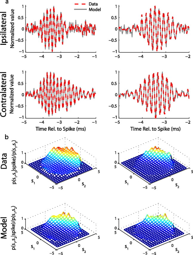
NL model components and recovery from model responses. a, Monaural STAs from collected responses (red dashed line) and model responses (gray line) to binaurally uncorrelated noise stimuli for two laminaris neurons. Rel., Relative. b, Estimates of the instantaneous probability of spiking given the monaural input signals for measured (Data) and model spikes (Model). Each plot is limited to ±4 SDs of the prior (see Materials and Methods). The model uses a quadratic input–output nonlinearity to map input signals to the spiking probability.
We estimated the input–output nonlinearity as f(s1, s2) = P(spike | s1, s2), where the input signals s1(t) = kL * sL(t) and s2(t) = kR * sR(t) are computed by convolving the left and right stimuli with their associated monaural filters. The signals s1 and s2 represent the fluctuations about the mean of the collective inputs from left and right afferent cochlear nucleus magnocellularis (NM) neurons, respectively. For all neurons, the highest probability of spiking occurred when both s1 and s2 are positive, corresponding to inputs at the preferred monaural phases and, therefore, coincident inputs. The dependence of spiking probability on s1 and s2 was an expansive nonlinear function (Fig. 5b), such that coincident inputs at the preferred monaural phases produce a higher spiking probability than the sum of the spiking probabilities when one signal is at the preferred phase and the other is 90° away from the preferred phase. We found that the structure of the instantaneous spiking probability is captured by modeling the input–output nonlinearity by a quadratic function (Eq. 2). The quadratic function is an expansive nonlinear function that includes a constant bias that is added to the sum of s1 and s2 before squaring. The DC bias reflects the high level of baseline firing in NM neurons and has the effect of producing a high spiking probability when both inputs are at the preferred phases and a low spiking probability when both inputs are away from the preferred phases. We first tested the quadratic model by recovering the monaural STAs and empirical spiking probability from model responses to novel stimuli. Both the monaural STAs (Fig. 5a) and the empirical spiking probability derived from the model spikes (Fig. 5b) had the same shapes as those computed from the NL data.
We examined ITD curves and phase locking of model neurons in response to novel stimuli. The shapes of the model and collected ITD curves were similar, including the location of the peaks in the ITD curve, the rate of decay at extreme ITDs, and the balance of binaural and monaural contributions to the shape of the tuning curve (Fig. 6). The mean difference between the ITD at the peak in the ITD curve nearest to 0 μs of experimental and model ITD curves over six neurons was 20 ± 15.5 μs, which is less than the ITD step size (30 μs). The experimentally measured and model-generated ITD tuning curves both display an ITD-independent component, as seen in the bias of the ITD curve (Fig. 6). The model ITD curves capture not only the ITD sensitivity about the mean, but also the relative strength of the ITD-independent component. The mean-squared correlation coefficient of the model-generated and the experimentally measured ITD tuning curves computed over an ITD range of ±1200 μs was 0.69 ± 0.11 (n = 6). Over the physiological range of ±250 μs (Keller et al., 1998; Poganiatz et al., 2001), the mean-squared correlation coefficient of the model-generated and the experimentally measured ITD tuning curves was 0.84 ± 0.05 (n = 6). Although ITD tuning was maintained in model responses as interaural level difference (ILD) varied, the model failed to produce the correct balance of monaural and binaural responses when ILD differed greatly from zero (data not shown). For example, monaural responses were well below the trough of the ITD tuning curve, which is in contrast to experimental observations (Viete et al., 1997).
Figure 6.

NL model responses to ITD. ITD curves for experimentally collected responses (black line) and model responses (gray line) for the two laminaris neurons shown in Figure 4. Error bars represent the SD. The vertical line indicates the estimated CD of the neuron.
Consistent with the cross-correlation model, the interaural difference between the average monaural phases of model responses to tones accurately predicted the CD of the neuron (Fig. 7d,h). The mean difference between the CD of the neuron and the prediction from the interaural difference in mean monaural phases of model neurons was 16.8 ± 9.9 μs (n = 6). The addition of a DC component to the filtered input signals before applying the squaring input–output nonlinearity (Eq. 2) removes a complication that is typically associated with modeling coincidence detector responses by a multiplicative operation. A strong argument against the use of a multiplicative mechanism to model coincidence detection can be found in the fact that the spikes of NL neurons are locked to the phase of the auditory stimulus (which explains the coherent STA in Fig. 2). Direct multiplication of the monaural input signals creates responses to binaural stimuli at multiple phases. However, by adding a DC bias to the monaural inputs before passing the input through a squaring nonlinearity, the NL model produced monaural and binaural phase histograms with single peaks (Fig. 7a–c,e–g).
Figure 7.

Phase locking by model NL neurons. a–c, e–g, Period histograms of model spiking responses for left (a, e), right (b, f), and binaurally (c, g) presented tones at the best frequency of the neuron for the two laminaris neurons shown in Figures 4 and 5. d, h, Experimentally measured ITD curve (solid line) along with the estimated CD of the neuron (vertical black line) and the predicted best ITD computed from the difference between the monaural mean phases (vertical dashed gray line).
Discussion
These results suggest that at the locus of computation of ITD in the barn owl the behavior of the coincidence detectors can be characterized as the cross-correlation between the stimuli presented to the two ears, up to a scaling factor and an offset. Consistent with the theory presented here, Yin et al. (1986) showed a correspondence between the sync-rate curve (the FTC weighted by a synchronization coefficient, which is the vector strength weighted by the firing rate) and the Fourier transform of the ITD curve. A direct comparison is difficult because Yin et al. (1986) did their work in the inferior colliculus, which receives inputs from and does not itself feature coincidence detector neurons (Shackleton et al., 2000), and spectral tuning was measured differently. However, it appears that their results are a close match for the FTC data presented here. Given that their sync-rate curve shares many of the limitations in estimating the effective frequency tuning using the FTC, it is possible that the relationship between spectral and ITD tuning also holds for the neurons they examined.
We show that the responses of coincidence detector neurons in NL are consistent with a linear-quadratic model. The model assumes that the filtered monaural input signals are reconstructed in the membrane potential and combined additively without distinguishing between left and right input spikes. ITD sensitivity arises because of the quadratic input–output property of the neuron. The existence of a quadratic mapping between membrane potentials and spikes in laminaris neurons may be simply attributable to noise in the subthreshold response (Hansel and van Vreeswijk, 2002; Miller and Troyer, 2002). Whereas the nature of the input–output properties of laminaris neurons remains an open question, such a power-law relationship between membrane potentials and spikes is evident in the owl's inferior colliculus (Peña and Konishi, 2002). The presence of a quadratic nonlinearity in the model was derived from the NL data and produces a response that is equal to the sum of the ideal cross-correlation of the filtered input signals, monaural terms, and a constant term as seen in the time average of the instantaneous spiking probability:
As shown in the simulations, the relationship between the ITD-dependent and -independent contributions to the response is as seen in the data. This is consistent with the observation of Batra and Yin (2004) that the neurons of MSO were more likely to be driven by coincidences because of synchronicity in the monaural afferents than predicted by an ideal cross-correlator. Although the model reproduces the observed ITD sensitivity of NL neurons for stimuli with zero ILD, the model fails to accurately describe the balance between monaural and binaural responses as the ILD deviates greatly from zero. The balancing of interaural intensity, thought to be accomplished via the superior olive (Viete et al., 1997), addresses this concern and may be included in a more detailed model as a gain control mechanism.
For perfect cross-correlation to take place in coincidence detector neurons, a representation of the effective monaural input must emerge in the membrane potential of coincidence detector neurons. The large number of NM axons connecting to each NL cell (Carr and Boudreau, 1993), coupled with the high spontaneous rate of NM neurons (Köppl, 1997), is consistent with a mechanism of convergence able to recreate an unrectified copy of the sound in NL neurons using only excitatory phase-locked inputs. The shape of the instantaneous spiking probability estimated from the NL data suggests that an unrectified representation of the effective monaural stimulus is reconstructed in the membrane potential. For each neuron, the spiking probability when one input is fixed at a high positive value is reduced as the contralateral effective input signal is decreased (Fig. 5b). The decrease in spiking probability continues as the input signal becomes negative, suggesting that the signal is not rectified. The reconstruction of the effective stimulus in the membrane potential has been predicted by models of the owl's NL as a sound-analog synaptic input being formed by phase-locked spikes of NM axons (Ashida et al., 2007).
Previous work has established that the coincidence detector neurons of the MSO (Yin and Chan, 1990) show behavior consistent with cross-correlation. However, it has also been shown that inhibition plays a critical role in determining the tuning to ITD (Brand et al., 2002). Although this inhibition seems to determine the location of the peak, it is not clear whether or not it distorts the overall shape of the rate-ITD function to an extent that would alter the linearity in the spectral domain between the input and the output of MSO neurons and therefore create deviations from the cross-correlation model. There is, at this point, no evidence that the barn owl uses inhibition to alter the shape of the rate-ITD functions of NL neurons; indeed, all evidence to date would seem to be consistent with the model of Jeffress (1948) (Carr and Konishi, 1990; Peña et al., 2001). By confirming that the ITD response of NL neurons is consistent with the cross-correlation theorem, we not only validate one of the key tenets of the Jeffress model but have set forth a methodology for examining this issue in other models in which the question remains open.
Footnotes
This work was supported by National Institutes of Health Grants DC00134 (M. Konishi) and DC007690 (J.L.P.). We thank M. Konishi for invaluable support and R. Lyon, P. Joris, P. Perona, and O. Schwartz for feedback.
References
- Ashida G, Abe K, Funabiki K, Konishi M. Passive soma facilitates submillisecond coincidence detection in the owl's auditory system. J Neurophysiol. 2007;97:2267–2282. doi: 10.1152/jn.00399.2006. [DOI] [PubMed] [Google Scholar]
- Batra R, Yin TCT. Cross correlation by neurons of the medial superior olive: a reexamination. JARO. 2004;5:238–252. doi: 10.1007/s10162-004-4027-4. [DOI] [PMC free article] [PubMed] [Google Scholar]
- Brand A, Behrend O, Marquardt T, McAlpine D, Grothe B. Precise inhibition is essential for microsecond interaural time difference coding. Nature. 2002;417:543–547. doi: 10.1038/417543a. [DOI] [PubMed] [Google Scholar]
- Carr CE, Boudreau RE. Organization of the nucleus magnocellularis and the nucleus laminaris in the barn owl: encoding and measuring interaural time differences. J Comp Neurol. 1993;334:337–355. doi: 10.1002/cne.903340302. [DOI] [PubMed] [Google Scholar]
- Carr CE, Konishi M. Axonal delay lines for time measurement in the owl's brainstem. Proc Natl Acad Sci U S A. 1988;85:8311–8315. doi: 10.1073/pnas.85.21.8311. [DOI] [PMC free article] [PubMed] [Google Scholar]
- Carr CE, Konishi M. A circuit for detection of interaural time differences in the brain stem of the barn owl. J Neurosci. 1990;10:3227–3246. doi: 10.1523/JNEUROSCI.10-10-03227.1990. [DOI] [PMC free article] [PubMed] [Google Scholar]
- Chichilnisky EJ. A simple white noise analysis of neural light responses. Network. 2001;12:199–213. [PubMed] [Google Scholar]
- Christianson GB, Peña JL. Preservation of spectrotemporal tuning between the nucleus laminaris and the inferior colliculus of the barn owl. J Neurophysiol. 2007;97:3544–3553. doi: 10.1152/jn.01162.2006. [DOI] [PMC free article] [PubMed] [Google Scholar]
- de Boer E, de Jongh HR. On cochlear encoding: potentialities and limitations of the reverse-correlation technique. J Acoust Soc Am. 1978;63:115–135. doi: 10.1121/1.381704. [DOI] [PubMed] [Google Scholar]
- Goldberg JM, Brown PB. Response of binaural neurons of dog superior olivary complex to dichotic tonal stimuli: some physiological mechanisms for sound localization. J Neurophysiol. 1969;32:613–636. doi: 10.1152/jn.1969.32.4.613. [DOI] [PubMed] [Google Scholar]
- Hansel D, van Vreeswijk C. How noise contributes to contrast invariance of orientation tuning in cat visual cortex. J Neurosci. 2002;22:5118–5128. doi: 10.1523/JNEUROSCI.22-12-05118.2002. [DOI] [PMC free article] [PubMed] [Google Scholar]
- Heffner RS, Heffner EH. Evolution of sound localization in mammals. In: Webster DB, Fay RR, Popper AN, editors. The evolutionary biology of hearing. New York: Springer; 1992. pp. 691–715. [Google Scholar]
- Jeffress LA. A place theory of sound localization. J Comp Physiol Psychol. 1948;41:35–39. doi: 10.1037/h0061495. [DOI] [PubMed] [Google Scholar]
- Joris P, Yin TCT. A matter of time: internal delays in binaural processing. Trends Neurosci. 2007;30:70–78. doi: 10.1016/j.tins.2006.12.004. [DOI] [PubMed] [Google Scholar]
- Keller CH, Takahashi TT. Representation of temporal features of complex sounds by the discharge patterns of neurons in the owl's inferior colliculus. J Neurophysiol. 2000;84:2638–2650. doi: 10.1152/jn.2000.84.5.2638. [DOI] [PubMed] [Google Scholar]
- Keller CH, Hartung K, Takahashi TT. Head-related transfer functions of the barn owl: measurement and neural responses. Hear Res. 1998;118:13–34. doi: 10.1016/s0378-5955(98)00014-8. [DOI] [PubMed] [Google Scholar]
- Köppl C. Frequency tuning and spontaneous activity in the auditory nerve and cochlear nucleus magnocellularis in the barn owl Tyto alba. J Neurophysiol. 1997;77:364–377. doi: 10.1152/jn.1997.77.1.364. [DOI] [PubMed] [Google Scholar]
- Licklider JCR. Three auditory theories. In: Koch S, editor. Psychology: a study of a science. New York: McGraw-Hill; 1959. pp. 41–144. [Google Scholar]
- McAlpine D, Jiang D, Palmer AR. A neural code for low-frequency sound localization in mammals. Nat Neurosci. 2001;4:396–401. doi: 10.1038/86049. [DOI] [PubMed] [Google Scholar]
- Miller KD, Troyer TW. Neural noise can explain expansive, power-law nonlinearities in neural response function. J Neurophysiol. 2002;87:653–659. doi: 10.1152/jn.00425.2001. [DOI] [PubMed] [Google Scholar]
- Moiseff A. Bi-coordinate sound localization by the barn owl. J Comp Physiol A Neuroethol Sens Neural Behav Physiol. 1989;164:637–644. doi: 10.1007/BF00614506. [DOI] [PubMed] [Google Scholar]
- Peña JL, Konishi M. From postsynaptic potentials to spikes in the genesis of auditory spatial receptive fields. J Neurosci. 2002;22:5652–5658. doi: 10.1523/JNEUROSCI.22-13-05652.2002. [DOI] [PMC free article] [PubMed] [Google Scholar]
- Peña JL, Viete S, Albeck Y, Konishi M. Tolerance to sound intensity of binaural coincidence detection in the nucleus laminaris of the owl. J Neurosci. 1996;16:7046–7054. doi: 10.1523/JNEUROSCI.16-21-07046.1996. [DOI] [PMC free article] [PubMed] [Google Scholar]
- Peña JL, Viete S, Funabiki K, Saberi K, Konishi M. Cochlear and neural delays for coincidence detection in owls. J Neurosci. 2001;21:9455–9459. doi: 10.1523/JNEUROSCI.21-23-09455.2001. [DOI] [PMC free article] [PubMed] [Google Scholar]
- Poganiatz I, Nelken I, Wagner H. Sound-localization experiments with barn owls in virtual space: influence of interaural time difference on head-turning behavior. J Assoc Res Otolaryngol. 2001;2:1–21. doi: 10.1007/s101620010039. [DOI] [PMC free article] [PubMed] [Google Scholar]
- Rose JE, Gross NB, Geisler CD, Hind JE. Some neural mechanisms in the inferior colliculus of the cat which may be relevant to localization of a sound source. J Neurophysiol. 1966;29:288–314. doi: 10.1152/jn.1966.29.2.288. [DOI] [PubMed] [Google Scholar]
- Seidl AH, Grothe B. Development of sound localization mechanisms in the mongolian gerbil is shaped by early acoustic experience. J Neurophyisol. 2005;94:1028–1036. doi: 10.1152/jn.01143.2004. [DOI] [PubMed] [Google Scholar]
- Shackleton TM, McAlpine D, Palmer AR. Modelling convergent input onto interaural-delay-sensitive inferior colliculus neurones. Hear Res. 2000;149:199–215. doi: 10.1016/s0378-5955(00)00187-8. [DOI] [PubMed] [Google Scholar]
- Spezio ML, Takahashi TT. Frequency-specific interaural level difference tuning predicts spatial response patterns of space-specific neurons in the barn owl inferior colliculus. J Neurosci. 2003;23:4677–4688. doi: 10.1523/JNEUROSCI.23-11-04677.2003. [DOI] [PMC free article] [PubMed] [Google Scholar]
- Viete S, Peña JL, Konishi M. Effects of interaural intensity difference on the processing of interaural time difference in the owl's nucleus laminaris. J Neurosci. 1997;17:1815–1824. doi: 10.1523/JNEUROSCI.17-05-01815.1997. [DOI] [PMC free article] [PubMed] [Google Scholar]
- Yang L, Monsivais P, Rubel EW. The superior olivary nucleus and its influence on nucleus laminaris: a source of inhibitory feedback for coincidence detection in the avian auditory brainstem. J Neurosci. 1999;19:2313–2325. doi: 10.1523/JNEUROSCI.19-06-02313.1999. [DOI] [PMC free article] [PubMed] [Google Scholar]
- Yin TCT, Chan JCK. Interaural time sensitivity in the medial superior olive of the cat. J Neurophysiol. 1990;64:465–488. doi: 10.1152/jn.1990.64.2.465. [DOI] [PubMed] [Google Scholar]
- Yin TCT, Kuwada S. Binaural interaction in low-frequency neurons in inferior colliculus of the cat. III. Effects of changing frequency. J Neurophysiol. 1983;50:1020–1042. doi: 10.1152/jn.1983.50.4.1020. [DOI] [PubMed] [Google Scholar]
- Yin TCT, Chan JCK, Irvine DRF. Effects of interaural time delays of noise stimuli on low-frequency cells in the cat's inferior colliculus. I. Responses to wideband noise. J Neurophysiol. 1986;55:280–300. doi: 10.1152/jn.1986.55.2.280. [DOI] [PubMed] [Google Scholar]
- Yin TCT, Chan JCK, Carney LH. Effects of interaural time delays of noise stimuli on low-frequency cells in the cat's inferior colliculus. III. Evidence for cross-correlation. J Neurosci. 1987;58:562–583. doi: 10.1152/jn.1987.58.3.562. [DOI] [PubMed] [Google Scholar]