Visual Estimation Under Risk

Abstract

We investigate whether observers take into account their visual uncertainty in an optimal manner in a perceptual estimation task with explicit rewards and penalties for performance. Observers judged the mean orientation of a briefly presented texture consisting of a collection of line segments. The mean and, in some experiments, the variance of the distribution of line orientations changed from trial to trial. Subjects tried to maximize the number of points won in a “bet” on the mean texture orientation. They placed their bet by rotating a visual display that indicated two ranges of orientations: a reward region and a neighboring penalty region. Subjects won 100 points if the mean texture orientation fell within the reward region, and lost points (0, 100 or 500, in separate blocks) if the mean orientation fell in the penalty region. We compared each subject's performance to a decision strategy that maximizes expected gain. For the nonzero-penalty conditions, this ideal strategy predicts subjects will adjust the payoff display to shift the center of the reward region away from the perceived mean texture orientation, putting the perceived mean orientation on the opposite side of the reward region from the penalty region. This shift is predicted to be larger for (1) larger penalties, (2) penalty regions located closer to the payoff region, and (3) larger stimulus variability. While some subjects' performance was nearly optimal, other subjects displayed a variety of suboptimal strategies when stimulus variability was high and changed unpredictably from trial to trial.

Introduction

Actions have consequences, and humans take those consequences into account in making decisions and planning actions. This issue pervades all human activity, whether it means choosing a curved path in reaching for the newspaper to avoid spilling the glass of juice that blocks the direct path, or leaving ten minutes earlier to reduce the possibility of missing a plane flight. In choosing the optimal course of action, one must combine uncertain sensory data, prior knowledge, variability in the outcomes of planned actions, and the costs and benefits of potential outcomes (Berger, 1985; Blackwell & Girshick, 1954; Ferguson, 1967).

In many experimental contexts, the subject's task is estimation (of depth, slant, location, orientation, etc.). In the absence of prior information or explicit consequences, subjects may attempt to maximize the percentage of correct responses, resulting in the adoption of a maximum-likelihood (ML) estimate to make optimum use of noisy sensory data (implicitly assuming a flat prior distribution). If one has prior information as to the probability of occurrence of different stimuli, one should combine that information with the sensory data (a Bayesian calculation), and use the maximum a posteriori (MAP) estimate (Kersten, Mamassian, & Yuille, 2004; Knill & Richards, 1996; Maloney, 2002; Mamassian, Landy, & Maloney, 2002). Finally, if there are known consequences (gains or losses) of different outcomes of the participant's decision or action, the optimal strategy (instead of optimizing percentage correct) is one that maximizes expected gain (MEG).

In rapid motor tasks under risk, subjects adopt strategies that are frequently indistinguishable from the optimal MEG solution. Trommershäuser, Maloney, and Landy (2003a,b) asked subjects to point rapidly at targets while avoiding nearby penalty regions. Hits on each region led to gains and losses that were known to the subject, and feedback was provided. Subjects were required to complete the movement in a short period of time, resulting in rapid, variable movements. Subjects adopted an aiming strategy that matched the MEG solution. They also modified their aim points appropriately when fingertip end point feedback was artificially altered to have increased variance, suggesting subjects estimated the uncertainty of their own movement outcomes (Trommershäuser et al., 2005).

The movement task under risk just described is analogous to traditional paper-and-pencil tasks (Maloney, Trommershäuser, & Landy, 2007; Trommershäuser, Landy, & Maloney, 2006). In these latter tasks, participants are presented with a set of lotteries and asked which they would prefer. Each lottery consists of a set of mutually exclusive outcomes, their values (e.g., in monetary gains or losses) and probability of occurrence. As an example, subjects might be asked to choose between lottery A: “You will receive $4 with probability .8, $0 otherwise”, and lottery B: “You will receive $3 for sure.” Participants often do not choose the lottery corresponding to MEG (Bell, Raiffa, & Tversky, 1988; Kahneman, Slovic, & Tversky, 1982; Kahneman & Tversky, 2000). These failures of the MEG model are often consistent with subjects having an exaggerated aversion to losses (Kahneman & Tversky, 1979) and exaggerating small probabilities (Allais, 1953; Attneave, 1953; Lichtenstein et al., 1978; Tversky & Kahneman, 1992).

Why do humans behave in a MEG-optimal fashion in a speeded reaching task, but suboptimally in a paper-and-pencil decision-making task? Weber, Shafir, and Blais (2004) suggest that human behavior (in particular, risk sensitivity) differs between tasks in which probabilities are implicit and learned from experience versus tasks in which probabilities are given explicitly (e.g., as a number, pie chart, etc.). In paper-and-pencil tasks, people generally overweight rare events, leading to the non-linear mapping from probabilities to decision weights in Prospect Theory (Kahneman & Tversky, 1979). Hertwig, Barron, Weber and Erev (2004) show that when probabilities are instead learned implicitly, subjects tend to underweight rare events due to undersampling (specific to their particular task) and recency effects. In the reaching task, the stochastic nature of outcomes is implicit (in the participant's sensory and motor uncertainty) whereas in the paper-and-pencil tasks, the probability is communicated explicitly. The experiments of Maloney et al. (2007) lend further support for this distinction. They added an explicit stochastic component to the speeded reaching task: The penalty and/or the reward were only awarded to the participant on 50% of the trials in which the corresponding regions were hit. This minor change to the procedure led to suboptimal aiming strategies.

In this paper, we present experiments that are formally analogous to those of Trommershäuser et al. (2003a,b), but in which subjects performed a purely perceptual task with no time constraints. In the movement task, movement variability limited performance. Here, visual estimation variability limited performance. Probabilities of each outcome were implicit (as they depended on the observer's sensory uncertainty), so that one might predict MEG-optimal behavior. But, this is not a rapid motor task; it is a slow, deliberate task. Thus, the cognitive nature of the task might instead result in suboptimal strategies as seen in paper-and-pencil decision-making tasks. We will determine whether subjects respond appropriately to changes of stimulus variability, which affects the MEG strategy. We find that some subjects did change strategy in response to changes in stimulus variability in a nearly optimal manner. But, unlike in the motor tasks, we found that many subjects did not adopt an ideal, MEG strategy when stimulus variability was high and varied from trial to trial.

General Methods

Apparatus

Most experiments were run at NYU on a Dell PC using a 17-inch Dell Ultrascan P780 flat screen Trinitron monitor viewed from a distance of 57 cm. The data for subject RG (an author) were collected at the Univ. of Glasgow on an Apple G3 computer using a 21-inch ViewSonic G220f monitor calibrated so that stimulus dimensions were identical. Experiments were run using the Psychophysics Toolbox (Brainard, 1997; Pelli, 1997).

Stimuli

The stimuli (Figure 1A-C) were textures consisting of a set of white line segments (.7 deg long, anti-aliased) on a gray background, randomly placed using a uniform distribution over a circle (diameter: 4.6 deg) at the center of the screen. The number of line segments was chosen randomly on each trial (mean: 39.4, SD: 6.3 lines). All lines fit entirely within the circular aperture. Lines that overlapped were summed and clipped at a contrast of 100%.

Figure 1.

Example stimuli and the four payoff displays. The top row contains example stimuli with s_l = .002 (A), .02 (B) and .2 (C). After a brief display of the stimulus, subjects were shown one of four possible payoff display in which the black, penalty region was either far from the white reward region (D-E) or near (F-G).

Line segment orientations were chosen randomly and independently based on a Von Mises distribution (Batschelet, 1981), a standard distribution on a circular variable (e.g., line orientation) analogous to the Gaussian distribution. It is defined as

$$M(\phi ;{\kappa }_l,{\theta }_l)=\frac{e^{{\kappa }_l\cos \left(2(\phi -{\theta }_l)\right)}}{\pi ∕(0,{\kappa }_l)},$$ (1)

where φ is the line orientation, θ_l is the circular mean orientation, κ_l is the concentration parameter, and I is the modified Bessel function. Note that this expression is slightly modified from the usual definition because the range of line orientation is from 0 to 180° while the usual formulation ranges from 0 to 360°. The concentration parameter κ_l is roughly analogous to inverse variance; the distribution is flat when κ_l = 0, and becomes narrower as κ_l increases. We will find it convenient to describe the distributions in terms of orientation variability or spread s_l = 1/κ_l. Figure 1 shows stimuli with spreads of .002 (Figure 1A), .02 (B) and .2 (C), spanning the entire range of s_l values used in this study. Treating this circular variable as if it were linear, these values of spread correspond to standard deviations of 1.3, 4.1 and 13.7°, respectively. On each trial, the mean orientation θ_l was chosen randomly and uniformly (from 0 to 180°). The manner in which s_l was chosen was different for each experiment and is described later.

Procedure

The task was a gambling game in which subjects “bet” on the mean orientation of stimulus textures. Each trial began with a fixation point displayed for 500 ms followed by the 1 s display of the stimulus. After the stimulus, a response display was shown (Figure 1D-G). The response display consisted of a pair of opposing white circular arcs delimiting the range of rewarded orientations, and outside and offset from that, a pair of black arcs delimiting the range of penalized orientations. The subject's task was to rotate the response display in increments of 1° using a pair of response keys until the mean line orientation θ_l fell within the reward range, but not within the penalty range. Subjects indicated they were satisfied with the setting by a key press. When θ_l fell within the reward range (i.e., a line with orientation θ_l through the center of the display intersected the white arcs as illustrated in Figure 2A), the subject was awarded 100 points. If θ_l fell within the penalty range, 0, 100 or 500 points were deducted (the penalty value was fixed within a block of trials, but varied across blocks). If θ_l fell within both the reward and penalty ranges, the subject received both the reward and penalty. Subjects were asked to try to win as many points as possible, i.e., to win rewards while avoiding penalties.

Figure 2.

Optimal task strategy. (A) For trials in which the penalty value was 0, the optimal strategy was to rotate the payoff display so that the center of the reward region was aligned with the mean orientation of the texture (indicated here by the black arrow). (B) In non-zero penalty conditions, as the task became more difficult due to higher penalty, increased spread s_l of stimulus line orientations, and/or decreased distance between the payoff and penalty regions, the optimal strategy required the observer to rotate the payoff display so as to move the penalty region further away from the mean texture orientation.

Both the reward and penalty ranges were 22° wide. There were two “Far” configurations (penalty range rotated 22° clockwise or counterclockwise from the reward range; Figure 1D-E) and two “Near” configurations (penalty offset 11° clockwise or counterclockwise from the reward; Figure 1F-G).

After indicating satisfaction with the setting, visual feedback was provided as to whether the mean orientation fell within the reward and/or penalty ranges. Subjects were never shown the mean orientation itself. Each block of trials began with a set of practice trials that resulted in visual feedback, but the points for these trials were not added to the cumulative score for the subject. At the end of each block of trials, the subject's cumulative score and earnings across blocks was displayed. In Experiment 3, most subjects ran three practice blocks with penalty set to zero to get used to the task.

Subjects

In Experiments 1 and 2, the subjects were either authors (MSL, JT, RG) or other members of the lab. These subjects merely competed for the best score. One undergraduate, DG, took part in Experiment 2 and was unaware of the purposes of the experiment or the specific optimal strategy appropriate for this task. In Experiment 3, one subject was aware of the conditions of the experiment (MSL). The other subjects in Experiment 3 were naive as to the purposes of the experiment. The naive subjects in Experiment 3 were paid $10/hour for participation plus a bonus of .025 cents/point. These performance bonuses ranged from a gain of $23.20 to a loss of $9.30 for one subject (we did not actually deduct this from the base pay for this one very suboptimal subject, but the subject wasn't aware of this while performing the task). Each block of trials took approximately 15 to 20 minutes to complete.

Data analysis

For each trial we recorded the mean orientation θ used to generate the stimulus, the orientation ψ of the payoff display chosen by the subject, and the score for that trial. The payoff display orientation was coded as the orientation of the line joining the centers of the two white reward arcs (which passed through the center of the display).

When the penalty value was zero, the optimal strategy was to rotate the payoff display to center the mean orientation of the stimulus in the reward region (Figure 2A). However, in the non-zero penalty conditions, as the task became more difficult due to increased penalty, increased spread s_l or decreased distance between the penalty and reward regions, subjects needed to rotate the payoff display to move the penalty further away from the mean stimulus orientation (Figure 2B). We recorded the shift δ of the setting ψ away from the mean orientation θ used to generate the texture. This shift was coded so that positive values indicate the subject set the orientation of the center of the penalty region on the opposite side of the reward region from the mean texture orientation (i.e., they “played it safe”). Thus, for the displays in Figure 1D,F, δ = θ−ψ, whereas in Figure 1E,G, δ = ψ−θ.

Circular statistics

In this paper, we use circular statistics (Batschelet, 1981) to describe both the generation of the stimuli and the distribution of subject responses. These are distributions of orientations that we model as a von Mises distribution just like our definition of the stimulus (Equation 1). The estimate of the mean of the distribution of shift settings, , was computed using the usual sample circular mean (Batschelet, 1981). The estimate of the concentration parameter was calculated using the procedure of Schou (1978). Schou showed that his procedure (a marginal-maximum-likelihood estimate) has lower bias than the ML procedure. The estimate of spread shown in the figures is simply . This is not the ML or marginal ML estimate of s_s, but bias should be low for the large number of trials contributing to each estimate.

In Experiments 1 and 2, for each value of s_l we used an estimate of (and ) that was pooled over the six conditions (three penalty levels and two types of configuration, Near and Far). Note that results were always pooled over the two mirror symmetric payoff displays by mirroring the data as discussed above in the definition of δ. Typical tests for equality of variance are based on the assumption that the underlying distributions are normal and are known to be sensitive to failures of the normality assumption (Keppel, 1982). Therefore, we devised a resampling method (Efron & Tibshirani, 1993) to test for the equality of the spreads over the six conditions based on an analogy to Hartley's F_max statistic (Keppel, 1982). We calculated the range of the six observed values (i.e., ). Then, we simulated the experiment 1000 times, assuming the pooled estimate of to be correct, and computed F_max for each set of six values. The p-value was estimated by determining the percentile of the observed F_max value in the distribution of simulated F_max values.

MEG predictions

In each experiment, we compare human performance to that of the MEG strategy. On each trial, the observer viewed a stimulus S that was generated based on line orientation distribution parameters θ_l and s_l, and one or both of these varied from trial to trial (with distributions that varied across the three experiments). The payoff displays in Figure 1D-G resulted in three regions with nonzero payoff: R₁ (reward only), R₂ (reward-penalty overlap) and R₃ (penalty only). The gain associated with the reward region G_r = 100 points; the gain associated with the penalty region G_r = 0, −100 or −500 points (depending on the block of trials).

The subject could not determine the precise value of θ_l; any estimate was corrupted by line segment orientation sample variability as well as any additional imprecision due to the observer's own sensory uncertainty or noisy calculations. The best the observer could do was, in each trial, to compute an estimate based on the stimulus and rotate the payoff display by an appropriate amount δ away from that orientation . Similarly, the subject could not know the value of s_l. The expected gain for any particular value δ was

$$\begin{array}{cc}\hfill \mathit{EG}\left(\delta \right)& =\int \int G(\delta \mid {\theta }_l)p({\theta }_l,s_l\mid S)d{\theta }_l{\mathit{ds}}_l\hfill \\ \hfill & =\int \int G(\delta \mid {\theta }_l)\frac{p(S\mid {\theta }_l,s_l)p({\theta }_l,s_l)}{p\left(S\right)}d{\theta }_l{\mathit{ds}}_l,\hfill \end{array}$$ (2)

where the gain depended only on δ and θ_l in our task. The MEG strategy was to choose the value of δ that maximized EG.

The strategy based on Equation 2 is an ideal MEG strategy in the sense that it presumes the subject can perfectly account for the likelihoods of various values of θ_l and s_l. But, subjects' settings were far more variable than this would predict. This was likely due to imperfect calculation of the mean orientation of the stimulus, variability in the calculation of the shift, imperfect memory of the mean stimulus orientation and/or variability due to imperfect adjustment of the response display. As one would expect, the spread of observer shift settings was a function of the spread of line orientations in the stimulus s_l. Thus, we were interested in a MEG model of performance based on a subject hampered by the setting variability we estimated from the subjects' settings. Once we had an estimate of observer setting spread , we had sufficient information to calculate the MEG settings. That is, the MEG model was determined entirely by the data and had no free parameters.

The calculation of this MEG strategy was analogous to that described by Trommershäuser et al. (2003a,b) except that here it took place on the circular domain of line orientation. The MEG strategy for this imperfect observer was analogous to that suggested by Equation 2 with the addition of subjects' setting variability beyond that implicit in the stimulus.

To determine the performance of this MEG model, we computed the performance of two simpler models. One was a supra-ideal model. It was supplied with more information about the stimulus than the subject could have known. Thus, its performance had to be as good or better than the MEG model. The other was a sub-ideal model. The performance of these two models brackets the predictions of the hard-to-compute MEG strategy.

For the supra-ideal strategy, we assumed that the model subject knew the correct value of the line orientation spread s_l used to generate the stimulus, and hence also knew the setting spread s_s. For this supra-ideal observer,

$$\mathit{EG}\left(\delta \right)=G_{r}P(R_1\mid \delta ,s_s)+(G_r+G_p)P(R_2\mid \delta ,s_s)+G_{p}P(R_3\mid \delta ,s_s).$$ (3)

The conditional probabilities in Equation 3 are simply integrals of the von Mises distribution over the intervals corresponding to each region for the candidate shift value δ. Again, the MEG strategy was to use the value of δ maximizing EG.

The sub-ideal observer was similar, except that rather than using the correct value s_l (that it couldn't have known), it used an estimate based on the spread of the line orientations in the stimulus shown on that trial . Otherwise, the computations were identical (i.e., it used instead of s_l to determine the value of s_s in Equation 3). We call this model sub-ideal, because it effectively skipped the step of integrating over s_l in Equation 2, using the estimate instead.

We simulated both the supra- and sub-ideal observers for all subjects for the results of Experiment 3 (with 1000 replications of the simulation for each observer). The performance of the two models was indistinguishable (data not shown here), and hence also indistinguishable from the optimal MEG performance bracketed by them. That is, any differences were clearly within the sampling noise of the simulations. Below, we use the supra-ideal model to compute the performance of the MEG strategy.

Efficiency

We define each observer's efficiency as the ratio of the number of points earned by the observer and the expected number of points that would have been earned had the observed used the MEG strategy in all conditions. This latter value was computed using estimated values based on that observer's data. This MEG observer model was simulated in the same experiment as the observer 1000 times to estimate a 95% confidence interval for the range of efficiencies the MEG observer was likely to generate (an interval that, by definition, was centered on 1.0). An observer was deemed significantly suboptimal if efficiency fell below this range. Note that here and elsewhere we do not perform Bonferroni corrections for multiple tests in computing error bars in each figure. Thus, the error bars reflect the variability of the simulations of that data point (i.e., they act like a typical standard error). Also, this leads to smaller error bars than would result from using the Bonferroni correction and thus makes is more likely that we will reject the null hypothesis that a subject is behaving optimally (i.e., in a sense, this is a conservative approach).

Deviation of mean settings from MEG predictions

In Experiments 1 and 2 we determined whether the mean shift for each condition was significantly different from the MEG shift for that subject in that condition. To do so, we performed 1000 simulations of that condition using the pooled value of (pooled over all penalty levels and Near/Far configurations for a given orientation spread and experiment; see Circular Statistics above) and the MEG strategy and determined a 95% confidence interval of MEG shift from the resulting distribution of mean shifts. The observer's mean shift value was deemed significantly different from the MEG strategy if it fell outside that interval (a 2-tailed test). We also plot error bars on the individual shifts. These were computed in the same way, using the observer's mean shift rather than the MEG shift for the simulations.

Deviation of points earned from MEG predictions

In Experiments 1 and 2 we also determine, for each subject and condition, whether the number of points earned was significantly different from that expected from the MEG strategy. To do so, we calculated a 95% confidence interval of points earned from the same simulations described above (i.e., using the pooled setting spreads and MEG strategy for that condition). The points earned by the observer in that condition were deemed significantly different from those expected from the MEG strategy if they fell outside that interval (a 2-tailed test). We also plot error bars on the individual numbers of points earned. These were computed similarly, using a new set of 1000 simulations using the observer's mean shift rather than the MEG shift. The position of these error bars is not guaranteed to be centered around the data points, and may even miss the data point completely. This happens if the distribution of settings used in the simulations differs substantially from the distribution of the setting data that led to that particular data point (especially in the high-penalty conditions, in which a small change in the number of penalties can lead to a large change in the score). Therefore, in the simulations used to compute these error bars, we used the setting spread estimated from the data in that condition alone, rather than the pooled setting spread. Nevertheless, in some conditions below the data points lie near or even beyond the ends of the error bars. This occured when the raw shift data for that condition were skewed, and hence poorly fit by the von Mises model of setting spread used in the simulations.

Experiment 1: Blocked Design

In this first experiment, both the penalty value and the orientation variability (i.e., s_l) were constant within a block. As shown below, subjects were highly efficient in terms of maximizing the number of points earned, although significantly suboptimal.

Methods

In this experiment, there were four conditions within each block of trials, corresponding to the four different reward/penalty configurations (Figure 1D-G). The reward value was 100 points; the penalty was 0, 100 or 500 points, varied between blocks. There were three levels of orientation variability corresponding to s_l values of .002 (least variable), .02 and .2 (most variable), also varied across blocks. Each block consisted of 20 practice trials (5 repeats of each configuration in random order), which did not impact the subject's cumulative score, followed by 80 trials (20 repeats of each configuration) that did add to the total score. Subjects ran three s_l = .002 blocks, then three s_l = .02 blocks, and finally three s_l = .2 blocks. Within each variability level, subjects ran one block with penalty 0, then one with penalty 100, and finally one with penalty 500. In other words, the blocks were run approximately in order from easiest to most difficult.

Results

For each subject and level of texture orientation variability, we examined the six concentration parameters κ_s of the six distributions of setting shifts δ corresponding to the different penalty values and the Near/Far configurations. For any given value of texture orientation variability, there was no pattern to the variation in the concentration parameters (i.e., subjects did not become more variable for more difficult conditions). The F_max statistic was significant (p<.05) for only three of the 15 such tests (five subjects, three levels of s_l, no Bonferroni correction was applied). Thus, we feel justified in computing a single pooled estimate of setting spread (the reciprocal of the pooled estimate ) for each subject and texture orientation variability s_l. These pooled setting spread values are shown in Figure 3. Clearly, increased stimulus variability led to increased setting variability. Also note that the setting spreads are far higher than the spread of the sample circular mean orientation from the ca. 40 lines in each stimulus, since the spread of the sample mean should be substantially smaller than the spread of the distribution used to select any single line orientation (i.e., the value on the abscissa). Thus, we are justified in including observer variability in the MEG model (Equation 3).

Figure 3.

Pooled setting spread as a function of texture orientation spread s_l for five subjects. Each value of was pooled across the three penalty levels and Near/Far configurations. Error bars are ±1 standard error computed using the 6 individual setting spreads that contributed to that pooled spread.

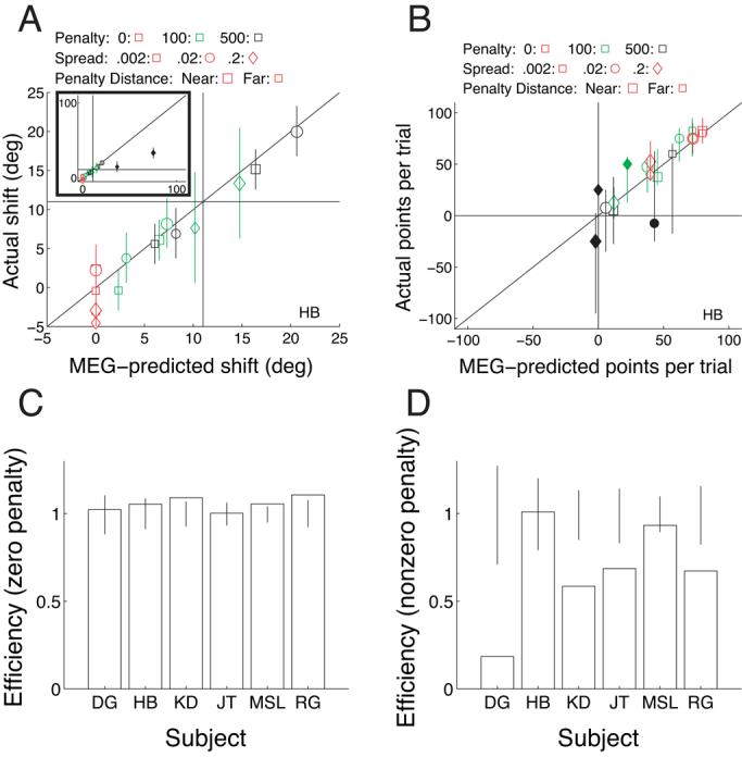
By and large, performance was good but significantly suboptimal. Figure 4A shows mean setting shifts (δ) as a function of the shift predicted by the MEG model for a typical subject (all other individual subject data are shown in Supplementary Figure A1). The MEG predictions were based on the variability of each subjects' settings (the pooled values) estimated from the data with no free parameters (Equation 3). Note that in most conditions, mean settings were not significantly different from MEG predictions (those that differed significantly are displayed with filled symbols). The horizontal and vertical lines on the plot represent the edge of the reward region (11 deg rotated from a zero shift, where zero represents the center of the reward region). The obvious suboptimal results (the two rightmost points) are conditions in which the MEG strategy required the subject to “aim” outside of the target region. All subjects were reticent to aim outside of the reward region when it was in their best interest to do so. This particular suboptimal strategy has also been noted in the reaching task (Trommershäuser et al., 2005).

Figure 4.

Results of Experiment 1. (A) Mean shift away from the penalty region is plotted as a function of the shift predicted by the optimal, MEG model for each condition (three penalty levels, Near and Far configurations, three level of stimulus orientation spread) for subject HB. The conditions are indicated by the symbol size (small symbols: Far penalty, large symbols: Near penalty), shape (squares: low orientation variability, circles: medium variability, diamonds: high variability), and color (red: penalty=0, green: penalty=100, black: penalty=500). Filled symbols indicate conditions in which the shift was significantly different from the MEG prediction. Error bars indicate 95% confidence intervals computed by bootstrap simulations. The diagonal line indicates perfect correspondence of data and prediction. The horizontal and vertical lines at a shift of 11 deg indicate the edge of the reward region. The inset shows the same data with expanded range on the axes to show the outlier. (B) Average number of points won per trial is plotted as a function of the MEG prediction for subject HB using the same conventions as in panel A. (C) Efficiency in the two zero-penalty conditions for five subjects. Error bars indicate the range of performance (95% confidence interval) expected from the MEG model. (D) Efficiency in the four nonzero-penalty conditions. Individual data for the other subjects are shown in Supplementary Figure A1

As a result of generally near-optimal aiming strategies, subjects' performance (in terms of the average number of points earned per trial) was also optimal or nearly so (Figure 4B). Note that occasionally an error bar in Supplementary Figure A1 does not overlap the point with which it corresponds. As pointed out in General Methods, this can occur because the distribution of settings in that particular condition was skewed and not well modeled by the von Mises distribution used in the simulations that generated the error bars.

The number of penalties awarded was highest when the penalty value was zero (Table 1). In this condition, there was no cost to hitting the penalty region, and so the optimal strategy was to aim at the center of the reward region, resulting in a relatively large number of penalties. As penalty value increased, subjects aimed further away from the penalty, reducing the number of penalties awarded. As spread decreased, setting spread also decreased, resulting in fewer penalties.

Table 1.

Penalties in Experiment 1

	Near Penalty				Far Penalty
Penalty	0	100	500	Avg	0	100	500	Avg	Overall
Spread
.002	59.0	29.0	10.5	32.8	7.0	2.0	2.5	3.8	18.3
.02	57.5	21.5	13.5	30.8	7.0	4.0	3.5	4.8	17.8
.2	48.5	26.0	16.5	30.3	16.5	11.0	13.0	13.5	21.9
Avg	55.0	25.5	13.5	31.3	10.2	5.7	6.3	7.4	19.4

Entries are the proportion of trials in each condition in which the setting fell within the penalty region, averaged over subjects.

Overall, efficiency was high (Figure 4C-D; the error bars are based on simulations of the MEG strategy). Figure 4C shows efficiency for the zero-penalty conditions alone, in which the MEG strategy was always to aim at the center of the reward region. Subjects successfully judged the mean orientation of the reward region in these conditions (Figure 4A). Unsurprisingly, for these conditions all subjects were optimal. Omitting these conditions and concentrating only on conditions requiring a nonzero shift, subjects all had high efficiency values (ranging from 61 to 81%; Figure 4D), but all were significantly suboptimal.

Experiment 2: Interleaved Design

In Experiment 1, subjects responded nearly optimally. That is, they shifted further away from the penalty range for large penalties and for textures with larger orientation variability. Inherent in such near-optimal behavior is the idea that subjects had a representation of their uncertainty in estimating the mean orientation of the texture stimulus and relied on this representation to set the orientation of the response display. It might be argued that this behavior was learned in the early trials of each block. In each block of trials there were only two reward/penalty configurations (pooling mirror-symmetric pairs together), and thus subjects were required to determine only two shift values. In Experiment 2, this strategy was made more difficult by changing the orientation variability trial by trial, thus mixing the three levels of orientation variability within each block of trials.

Methods

In this experiment, there were 12 conditions within each block of trials, corresponding to combinations of the four different reward/penalty configurations and three levels of orientation variability. The reward value was again 100 points; the penalty was 0, 100 or 500 points, varied between blocks. Each block consisted of 24 practice trials (2 repeats of each condition in random order), which did not impact the subject's cumulative score, followed by 120 trials (10 repeats of each condition) that did add to the total score. Subjects ran six blocks with penalty set to 0, 100, 500, 0, 100 and 500, respectively.

Results

Again, we examined the individual κ_s values. This time there was some hint that setting spreads increased with task difficulty, but the F_max test was significant for only five tests out of 18 (six subjects, three texture orientation spreads, no Bonferroni correction was applied). Results for a typical subject are shown in Figure 5A-B in the same format as Figure 4 (all other individual subject data are shown in Supplementary Figure A2. The mixed-block design of Experiment 2 presented no additional difficulty for this subject. The proportion of penalties awarded in each condition is shown in Table 2 and are similar to the results in Experiment 1. Efficiency values are shown in Figure 5C-D in the same format as Figure 4. Again, all subjects were optimal in the zero-penalty conditions. For most subjects, efficiency was also high in the nonzero-penalty conditions (Figure 5D), except for the most variable subject (DG).

Figure 5.

Results of Experiment 2. All plotting conventions as in Figure 4. (A) Setting shifts. (B) Performance in points per trial. (C) Efficiency in the two zero-penalty conditions. (D) Efficiency in the four nonzero-penalty conditions. Individual data for the other subjects are shown in Supplementary Figure A2.

Table 2.

Penalties in Experiment 2

	Near Penalty				Far Penalty
Penalty	0	100	500	Avg	0	100	500	Avg	Overall
Spread
.002	54.6	24.2	10.0	29.6	9.6	3.8	3.8	5.7	17.6
.02	53.8	25.8	14.6	31.4	11.2	5.4	5.8	7.5	19.4
.2	52.1	24.2	17.1	31.1	22.1	14.2	6.7	14.3	22.7
Avg	53.5	24.7	13.9	30.7	14.3	7.8	5.4	9.2	19.9

Entries are the proportion of trials in each condition in which the setting fell within the penalty region, averaged over subjects.

Experiment 3: Continuous Visual Variability

In Experiment 2 we varied stimulus variability randomly on a trial-by-trial basis and found that most subjects were again good at compensating for the amount of stimulus variability, resulting in task strategies with high efficiency. Thus, they reacted to changes in the amount of penalty and the degree of orientation variability appropriately, shifting away from the penalty region more (in non-zero penalty conditions) with increasing penalty, increased stimulus variability, and closer penalty regions.

In Experiment 3 we decided to test further whether subjects accurately account for the amount of stimulus variability. In Experiment 2 there were three discrete levels of orientation variability (Figure 1A-C), and these were easily discriminable. On each trial subjects recognized immediately whether it was a difficult or an easy trial (in terms of accuracy at estimating mean orientation). In Experiment 3 the orientation variability was chosen from a continuous, uniform distribution of spread values over the same range used in Experiments 1 and 2. Thus, subjects were forced to account for the particular amount of uncertainty on each trial to determine the appropriate shift. We mainly used naive subjects in Experiment 3 that were new to the task, i.e. they had not participated in Experiments 1 or 2, so they could not have been extending strategies learned in those experiments.

Methods

In this experiment, there were 4 conditions within each block of trials, corresponding to the four different reward/penalty configurations. The orientation variability was chosen randomly on each trial. In a pilot experiment, we determined that estimated setting spread was approximately a linear function of line orientation spread s_l. Therefore, in the experiment the line orientation spread s_l was chosen uniformly over the range [.002,.2]. This procedure led to a fairly uniform distribution of difficulty, and hence of optimal shift. The reward value was again 100 points; the penalty was 0, 100 or 500 points, varied between blocks. Each block consisted of 24 practice trials (6 repeats of each condition in random order), which did not impact the subject's cumulative score, followed by 120 trials (30 repeats of each condition) that did add to the total score. Most subjects ran three full practice blocks with penalty 0, followed by 12 blocks with penalty taking the values 0, 100, 500, repeated in sequence. Subject MSL ran 9 scored blocks.

Results

In the non-zero penalty conditions, no subject used an optimal strategy. We begin by examining the data of the one non-naive subject (MSL) to indicate what nearly optimal performance would look like. We then discuss how the performance of the naive subjects differed from this.

Figure 6 shows the raw data for subject MSL (an author; the full raw datasets for the 9 naive subjects are shown in Supplementary Figure A3). There are six panels corresponding to the three penalty levels (varied between blocks) and the Near/Far configurations (mixed within each block). Setting shift is plotted as a function of stimulus orientation spread. On each plot, the horizontal colored bars indicate the range of orientations corresponding to the reward (light green) and penalty (dark red) regions. These regions overlapped in the Near configuration, as indicated by the light green/dark red stripes. Thus, when a setting landed in the light green, there was a reward. When it landed in the red, a penalty was incurred. When it fell in the striped region, both the reward and penalty were given. The variability of responses increases with increase in stimulus spread (i.e., from left to right in each plot) as in Experiments 1 and 2 (e.g., Figure 3). The amount of shift upward (away from the penalty region) was zero in the zero-penalty conditions, but increased with increasing penalty, with increasing stimulus orientation spread, and with the Near configuration. All of this is qualitatively consistent with Experiments 1 and 2 and the MEG predictions.

Figure 6.

Settings in Experiment 3 for subject MSL. Individual shifts are plotted as a function of stimulus orientation spread for the six conditions (three penalty levels, Near and Far configurations). The light green bar indicates the reward region. The dark red bar indicates the penalty region. The striped area for the Near configurations indicates the range of orientations where the penalty and reward regions overlapped. Data for the other subjects are shown in Supplementary Figure A3.

The spread of responses for subject MSL is shown in Figure 7 (other subjects' data are shown in Supplementary Figure A4). The setting spread was computed by binning the data (bin width = .04). Again, there was a tendency for increasing setting spread with increasing stimulus orientation spread, as expected. We fit a line to the data pooled over the two zero-penalty conditions, plotted as the dashed line in all six panels. There was a tendency for setting spread to increase above this line in the 500-penalty conditions.

Figure 7.

Setting spreads in Experiment 3 for subject MSL. Setting spreads are plotted as a function of stimulus orientation spread for the six conditions, computed using bins of width 0.4. Dashed lines show a linear fit to the data pooled over the two zero-penalty conditions. Data for the other subjects are shown in Supplementary Figure A4.

Figure 8 shows the setting shifts (solid line) and the MEG predictions (dashed line) as a function of stimulus orientation spread (binned with bin width .04; all other subjects' data are shown in Supplementary Figure A5). The MEG predictions were derived based on the straight line fit to the zero-penalty conditions in Figure 7 as this yielded the best estimate of the lowest setting spread of which this subject was capable. That is, the increase in setting spread with higher penalties must have been a result of a variable strategy, rather than sensory variability. The mean shifts were close to the optimal strategy, although there was a tendency to undershift in the high-penalty conditions.

Figure 8.

Average setting shifts in Experiment 3 for subject MSL. Setting shifts are plotted as a function of stimulus orientation spread for the six conditions, computed using bins of width 0.4 (solid lines). Dashed lines indicate the MEG predictions based on the linear fit to the setting spread data shown as the dashed lines in Figure 7. Shaded areas indicate the reward and penalty regions as in Figure 6. Data for the other subjects are shown in Supplementary Figure A5.

Figure 9 shows the overall efficiency for MSL and for the 9 naive subjects in the zero- and nonzero-penalty conditions. MSL's strategy was nearly optimal (Figure 8), and hence his efficiency was close to one. Although a few of the other subjects achieved high efficiencies in the nonzero-penalty conditions, several subjects' efficiencies were substantially lower than those in Experiments 1 and 2. Four out of nine naive subjects lost points in the nonzero-penalty conditions, and one subject (SMN) managed to lose points overall. (Note that subject AVP's efficiency for the zero-penalty case was significantly greater than one due to outliers in the setting data leading to an inflated estimate of AVP's setting variability.)

Figure 9.

Efficiency values for all subjects in Experiment 3. (A) Zero-penalty conditions. (B) Nonzero-penalty conditions. Note that panel (B) has a different y-axis scale and a break in the axis to accommodate the poor performance of subject SMN. Error bars indicate the range of performance (95% confidence interval) expected from the MEG model.

This large range of efficiencies was apparently due to differences in the strategies subjects adopted. The four strategies that we found are illustrated in Figure 10, which shows raw data for four subjects in two conditions (Penalty 0, Far; Penalty 500, Near). Subject AT used a near-optimal strategy in the Penalty 0 and 100 conditions. But when the penalty value was 500, this subject played it safe by simply shifting so as to avoid the penalty (all trials with the Near configuration, fewer with the Far configuration). This turned out to be an excellent strategy, as the possible MEG in these conditions is low, and suboptimal strategies can be costly. As a result (and with some luck), AT achieved a fairly high efficiency. Subject AVP (along with AEW, AKK and ST) responded with random shifts (that appear to be uniform over the entire range of possible shifts) whenever the task became difficult (high penalty, Near configuration and/or high stimulus orientation spread). Subjects MHF and MMC used a bimodal strategy for which shifts were either near zero (aiming at the target) or 80-85° (aiming away from the penalty), with the avoidance strategy predominating for the more difficult conditions (leading to high efficiency for MMC, who avoided the penalty primarily in the most difficult conditions). Finally, subjects SMN and SF never figured out how to handle the penalty region, and always aimed at the center of the target region, although their setting spread increased substantially in the more difficult conditions. These differences in strategy led to very different proportions of penalties awarded (Table 3. These proportions are consistent with the observers' efficiency at performing the task.

Figure 10.

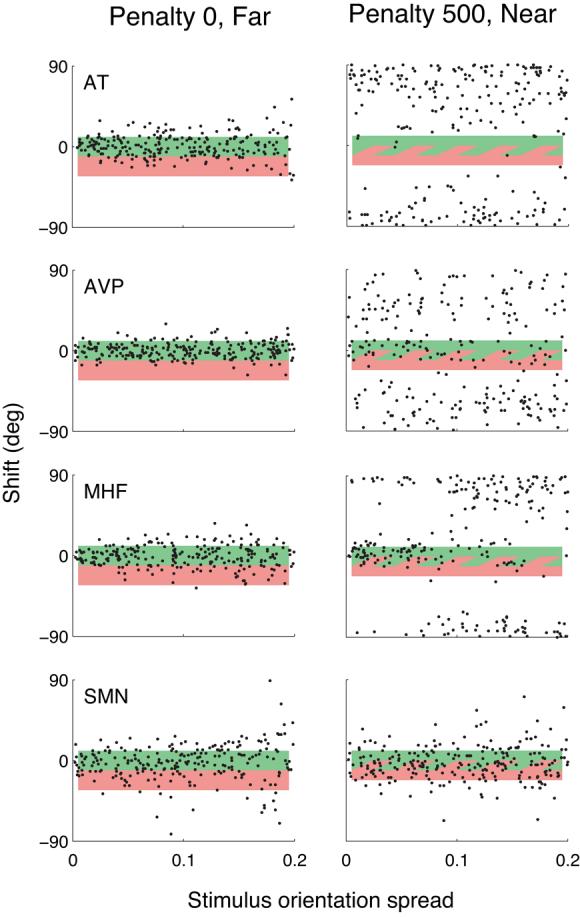
Settings in Experiment 3 for four subjects in two conditions (Penalty 0, Far; Penalty 500, Near). Plotting conventions as in Figure 6.

Table 3.

Penalties in Experiment 3

	Near Penalty				Far Penalty
Penalty	0	100	500	Avg	0	100	500	Avg	Overall
Spread
AEW	46.2	48.3	32.1	42.2	18.8	17.1	20.4	18.8	30.5
AKK	51.7	28.3	8.3	29.4	24.2	12.1	8.3	14.9	22.2
AT	47.5	26.7	0.8	25.0	17.1	13.8	6.2	12.4	18.7
AVP	52.1	52.1	14.2	39.4	8.8	12.5	10.4	10.6	25.0
MHF	44.2	36.2	15.4	31.9	20.4	13.3	7.9	13.9	22.9
MMC	47.1	36.7	9.6	31.1	14.6	9.6	3.8	9.3	20.2
MSL	56.1	30.6	9.4	32.0	12.2	8.3	4.4	8.3	20.2
SF	31.2	30.8	21.2	27.8	17.5	12.5	15.8	15.3	21.5
SMN	45.8	39.6	48.4	44.7	23.8	30.8	25.4	26.7	35.7
ST	46.2	35.8	19.6	33.9	21.7	19.6	19.6	20.3	27.1
Avg	46.6	36.7	18.2	33.8	18.0	15.1	12.4	15.2	24.5

Entries are the proportion of trials in each condition in which the setting fell within the penalty region, averaged over subjects and noise levels.

In summary, although two subjects (MSL, MMC) chose strategies nearly indistinguishable from the MEG-optimal solutions, the majority of subjects failed to do so. Instead, they adopted a variety of strategies including the effective, avoid-the-penalty strategy of subject AT as well as other, more costly approaches.

Discussion

We have presented data from three experiments in which subjects made perceptual judgments under risk. We find that subjects varied their strategy as a function of stimulus (and hence sensory) variability. In some cases and for some subjects, strategies were used that were MEG-optimal or nearly so over a wide range of stimulus conditions. But, performance dropped below optimal under conditions of high stimulus spread or if stimulus spread varied from trial to trial over a continuous range of spread values.

In the latter conditions (Experiment 3), there was a great deal of inter-subject variability. Subjects adopted a variety of sub-optimal strategies. In these conditions, some subjects aimed at the center of the target region despite the nearby, high-cost penalty region. Others switched between aim-at-the-target and avoid-the-penalty strategies. Other subjects never figured out a useful strategy at all, and their settings became random in these more difficult conditions.

What are the conditions under which nearly optimal behavior is obtained? Consistent with the results of our previous reaching studies, it seems that subjects perform worse when optimal behavior includes aiming outside of the reward region (Trommershäuser et al., 2005) or the stochastic nature of the task is made explicit (Maloney et al., 2007; see also Hertwig et al., 2004; Weber et al., 2004). The current task was also more difficult due to its memory requirements. Subjects had to remember the mean orientation of the stimulus after it disappeared while adjusting the response display.

Optimal behavior in our task required subjects to choose a shift that depended on both the mean and the spread of orientations in the stimulus. Actually, this optimal shift depended on the setting spread, which resulted from line orientation spread as well as response variability due to errors in calculating the mean orientation or in adjusting the payoff display.

There is evidence from the literature on visual texture perception that stimulus orientation variability is represented in the human visual system. Two line textures differ in appearance when the mean orientations or orientation spreads differ sufficiently. Two such neighboring textures segregate perceptually. Dakin (2001) analyzed the sources of uncertainty in the coding of mean orientation and Dakin and Watt (1997) also noted observers' ability to discriminate textures based on orientation variability. A region-based mechanism is used for segregating textures based on differences in orientation spread as if one were, indeed, calculating the orientation spread of each constituent texture (Wolfson & Landy, 1998). A better understanding of the mechanisms and sources of noise in coding texture orientation would help refine models of performance in tasks such as ours.

References

- Allais M. Le comportment de l'homme rationnel devant la risque: critique des postulats et axiomes de l'école Américaine. Econometrica. 1953;21:503–546. [Google Scholar]
- Attneave F. Psychological probability as a function of experienced frequency. Journal of Experimental Psychology. 1953;46:81–86. doi: 10.1037/h0057955. [DOI] [PubMed] [Google Scholar]
- Batschelet E. Circular statistics in biology. Academic Press; New York: 1981. [Google Scholar]
- Bell DE, Raiffa H, Tversky A, editors. Decision making: descriptive, normative and prescriptive interactions. Cambridge University Press; Cambridge, UK: 1988. [Google Scholar]
- Berger JO. Statistical decision theory and Bayesian analysis. 2nd ed. Springer; NY: 1985. [Google Scholar]
- Blackwell D, Girshick MA. Theory of games and statistical decisions. Wiley; NY: 1954. [Google Scholar]
- Brainard DH. The psychophysics toolbox. Spatial Vision. 1997;10:433–436. [PubMed] [Google Scholar]
- Dakin SC. Information limit on the spatial integration of local orientation signals. Journal of the Optical Society of America A. 2001;18:1016–1026. doi: 10.1364/josaa.18.001016. [DOI] [PubMed] [Google Scholar]
- Dakin SC, Watt RJ. The computation of orientation statistics from visual texture. Vision Research. 1997;37:3181–3192. doi: 10.1016/s0042-6989(97)00133-8. [DOI] [PubMed] [Google Scholar]
- Efron B, Tibshirani R. An Introduction to the Bootstrap. Chapman-Hall; New York: 1993. [Google Scholar]
- Ferguson TS. Mathematical statistics: a decision theoretic approach. Academic Press; NY: 1967. [Google Scholar]
- Hertwig R, Barron G, Weber EU, Erev I. Decision from experience and the effect of rare events in risky choice. Psychological Science. 2004;15:534–539. doi: 10.1111/j.0956-7976.2004.00715.x. [DOI] [PubMed] [Google Scholar]
- Kahneman D, Slovic P, Tversky A, editors. Judgment under uncertainty: heuristics and biases. Cambridge University Press; Cambridge, UK: 1982. [DOI] [PubMed] [Google Scholar]
- Kahneman D, Tversky A. Prospect Theory: An analysis of decision under risk. Econometrica. 1979;47:263–291. [Google Scholar]
- Kahneman D, Tversky A, editors. Choices, values & frames. Cambridge University Press; New York: 2000. [Google Scholar]
- Keppel G. Design and analysis: A researcher's handbook. 2nd Ed. Prentice-Hall; Englewood Cliffs, NJ: 1982. pp. 97–99. [Google Scholar]
- Kersten D, Mamassian P, Yuille A. Object perception as Bayesian inference. Annual Review of Psychology. 2004;55:271–304. doi: 10.1146/annurev.psych.55.090902.142005. [DOI] [PubMed] [Google Scholar]
- Knill DC, Richards W. Perception as Bayesian inference. Cambridge University Press; Cambridge, UK: 1996. [Google Scholar]
- Lichtenstein S, Slovic P, Fischhoff B, Layman M, Coombs B. Judged frequency of lethal events. Journal of Experimental Psychology: Human Learning and Memory. 1978;4:551–578. [PubMed] [Google Scholar]
- Maloney LT. Statistical decision theory and biological vision. In: Heyer D, Mausfeld R, editors. Perception and the physical world: psychological and philosophical issues in perception. Wiley; New York: 2002. pp. 145–189. [Google Scholar]
- Maloney LT, Trommershäuser J, Landy MS. Questions without words: A comparison between decision making under risk and movement planning under risk. In: Gray W, editor. Integrated models of cognitive systems. Oxford University Press; New York: 2007. in press. [Google Scholar]
- Mamassian P, Landy MS, Maloney LT. Bayesian modeling of visual perception. In: Rao RP, Olshausen BA, Lewicki MS, Rao RP, Olshausen BA, Lewicki MS, editors. Probabilistic models of the brain: perception and neural function. MIT Press; Cambridge, MA: 2002. pp. 13–36. [Google Scholar]
- Pelli DG. The VideoToolbox software for visual psychophysics: Transforming numbers into movies. Spatial Vision. 1997;10:437–442. [PubMed] [Google Scholar]
- Schou G. Estimation of the concentration parameter in von Mises-Fisher distributions. Biometrika. 1978;65:369–377. [Google Scholar]
- Trommershäuser J, Landy MS, Maloney LT. Humans rapidly estimate expected gain in movement planning. Psychological Science. 2006;17:981–988. doi: 10.1111/j.1467-9280.2006.01816.x. [DOI] [PubMed] [Google Scholar]
- Trommershäuser J, Maloney LT, Landy MS. Statistical decision theory and tradeoffs in motor response. Spatial Vision. 2003a;16:255–275. doi: 10.1163/156856803322467527. [DOI] [PubMed] [Google Scholar]
- Trommershäuser J, Maloney LT, Landy MS. Statistical decision theory and rapid, goal-directed movements. Journal of the Optical Society A. 2003b;20:1419–1433. doi: 10.1364/josaa.20.001419. [DOI] [PubMed] [Google Scholar]
- Trommershäuser J, Gepshtein S, Maloney LT, Landy MS, Banks MS. Optimal compensation for changes in task-relevant movement variability. Journal of Neuroscience. 2005;25:7169–7178. doi: 10.1523/JNEUROSCI.1906-05.2005. [DOI] [PMC free article] [PubMed] [Google Scholar]
- Tversky A, Kahneman D. Advances in prospect theory: cumulative representation of uncertainty. Risk and Uncertainty. 1992;5:297–323. [Google Scholar]
- Weber EU, Shafir S, Blais A-R. Predicting risk-sensitivity in humans and lower animals: Risk as variance or coefficient of variation. Psychological Review. 2004;111:430–445. doi: 10.1037/0033-295X.111.2.430. [DOI] [PubMed] [Google Scholar]
- Wolfson SS, Landy MS. Examining edge- and region-based texture mechanisms. Vision Research. 1998;38:439–446. doi: 10.1016/s0042-6989(97)00153-3. [DOI] [PubMed] [Google Scholar]
Associated Data
This section collects any data citations, data availability statements, or supplementary materials included in this article.