

Abstract
Computer simulations have become an invaluable tool to study the sometimes counterintuitive temporal dynamics of (bio-)chemical systems. In particular, stochastic simulation methods have attracted increasing interest recently. In contrast to the well-known deterministic approach based on ordinary differential equations, they can capture effects that occur due to the underlying discreteness of the systems and random fluctuations in molecular numbers. Numerous stochastic, approximate stochastic and hybrid simulation methods have been proposed in the literature. In this article, they are systematically reviewed in order to guide the researcher and help her find the appropriate method for a specific problem.
Keywords: stochastic simulation, biochemical systems, approximate stochastic simulation, hybrid simulation methods, systems biology
I have come to believe that one's; knowledge of any dynamical system is deficient unless one knows a valid way to numerically simulate that system on a computer.
Daniel T. Gillespie
INTRODUCTION
Biochemical networks, such as metabolism, signaling pathways or gene regulation, are characterized by a vast degree of interaction between many heterogeneous components. Often this results in complex temporal behavior that is difficult to comprehend. Therefore, computer simulations reproducing the dynamics of these systems have become an essential tool for researchers in the field [1, 2].
In most cases these simulations are based on deterministic modeling. Here, the systems are assumed to be continuous and to evolve deterministically. Their change over time can be described using ordinary differential equations (ODEs) [3]. The ODEs can then be solved by numerical integration to yield the dynamics of the system, and many efficient algorithms for that can be found in the literature, e.g. [4]. Since in the ODE approach, the biochemical systems are modeled as being continuous and deterministic, phenomena that occur due to the underlying discreteness of the systems and random fluctuations in molecular numbers, particularly in subsystems containing only few particles, are neglected.
Already in the 1970s stochastic algorithms have been devised that are able to account for fluctuations in discrete particle numbers [5] (the relationship between stochastic and deterministic models is studied in [6, 7]). However, these methods can be computationally demanding, and, therefore, numerous different (optimized/approximate/hybrid) stochastic algorithms have been developed recently in order to speed up the calculation.
The present article provides a systematic and comprehensive overview of the different stochastic simulation methods in order to help researchers seeking the appropriate method for their problem (see also [8–9]).
It should be mentioned that this review will be concerned with spatially homogeneous models only. When the spatial organization of biochemical systems should be taken into account, one has to resort to spatio-temporal simulation algorithms. For brief reviews on stochastic spatial approaches see e.g. [11–14]. Software capable of handling spatial models include, e.g. MCell [15, 16], MesoRD [17–19], Smoldyn [20, 21] or SmartCell [22, 23].
STOCHASTIC SIMULATIONS: ASSETS AND DRAWBACKS
Even though the deterministic approach has proven very successful, it comes with some issues:
Small particle numbers in cellular subsystems (e.g. in signaling pathways) lead to random fluctuations which can change the dynamic behavior considerably [24].
Bi- or multi-stable systems can not be described adequately [25].
Stochasticity itself can be an important property of the system, e.g. in evolution, noise-induced amplification of signals or noise-driven divergence of cell fates (for a review see [26]).
For very small particle numbers (e.g. single genes) the concept of continuous concentrations is not appropriate [27].
Inherent stochastic fluctuations in molecule numbers can change the dynamic behavior of biochemical systems both quantitatively and qualitatively [28, 29]. One example is the production of proteins in random bursts [24]. Another example is the lysis/lysogeny switch in λ-phage-infected Escherichia coli cells [25]. This is not restricted to systems containing low-numbered species, but can also happen in systems particularly sensitive to noise or operating near a bifurcation point [30, 27].
Cells must act in a coordinated way despite ubiquitous molecular noise. Therefore, specific cellular systems to cope with or even exploit stochastic effects are likely to be very important and deserve further study. Stochastic modeling provides the appropriate framework to investigate, for example, the robustness of cells against random perturbations [31–38] or the constructive effects of noise [25, 39–41].
In all the above cases, random fluctuations in discrete particle numbers should be accounted for and stochastic modeling and simulation is required.
Noise can even help with elucidating the functioning of biochemical systems. Examples where noise is exploited to study the underlying cellular processes include [42–44].
However, stochastic simulations usually are much more computationally demanding than deterministic methods. Exact methods take time proportional to the number of single reaction events occurring during the simulation time.
One other drawback of stochastic modeling is that it still lacks behind in terms of appropriate analysis methods, such as stochastic bifurcation analysis [45], stochastic Metabolic Control Analysis (MCA) [46] or stochastic sensitivity analysis [47].
Now, the practical question arises when stochastic simulation should be preferred over numerical integration of ODEs for a specific system one wants to analyze. Definite indicators necessitating stochastic modeling are (i) when the particle numbers are in a range where the concept of continuous concentrations is no longer appropriate, or (ii) when phenomena associated with stochasticity itself are the object of research. Beyond that most often rules of thumb based on the rough particle numbers in the system have been used to answer the question. This heuristic can be justified by the asymptotic equivalence of the Master Equation and the chemical Langevin equation (see Langevin method section) and the observation that often the relative magnitude of random fluctuations is inversely proportional to the square root of the system's; particle numbers [26]. However, giving a general threshold for the particle numbers, above which it is safe to employ deterministic methods, is surely impossible. The emergence of stochastic effects is very model-dependent and this has to be checked in each individual case [30, 27].
STOCHASTIC SIMULATION METHODS
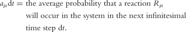
The stochastic approaches are based on the notion of a stochastic reaction constant cμ for each reaction Rμ in the system. cμ is the average probability that a specific combination of substrate particles in the system will react in the next infinitesimal time step dt according to reaction Rμ. Multiplied with the number of possible Rμ substrate particle combinations hμ (see [5] for details) we get a propensity aμ for reaction Rμ as aμ = hμcμ with:
 |
(1) |
aμ can be derived from the conventional deterministic reaction rate in the case of mass action kinetics.
It turns out that within this framework, the biochemical system can be identified with a (homogeneous) jump-type Markov process represented by a so-called Chemical Master Equation (CME) [5, 48], which describes the time evolution of the system state probability distribution. In general, this differential-difference equation is infinitely dimensional. Solving it, either analytically or numerically, still is a challenging task (the interested reader is refered to [49–51]). Therefore, one resorts to stochastic simulation methods that, using Monte Carlo calculation schemes, generate instances of the underlying stochastic process according to the Master Equation. However, since each run yields only one single trajectory, several runs have to be computed to be able to calculate statistics.
Stochastic simulation algorithms (SSA) can roughly be divided into exact, approximate or hybrid methods depending on whether or not they introduce approximations or combine different approaches into one calculation scheme.
EXACT STOCHASTIC METHODS
The so-called exact stochastic methods correctly account for inherent stochastic fluctuations and correlations. In addition, the discrete nature of the system is considered. Hence, they remain valid for very small particle numbers.
However, since they explicitly simulate each reaction event in the system, they have time complexity approximately proportional to the overall number of particles  present in the system. Therefore, they are prohibitively slow on large systems.
Gillespie [5] proposed two simple SSA, namely the Direct Method and the First Reaction Method. They are based on the so-called Reaction Probability Density Function:
 |
(2) |
This function determines the probability P(τ,μ|x,t)dτ that starting in state x at time-point t the next reaction in the system will occur in the time interval [t + τ,t + τ + dτ] and will be of type Rμ. The reaction times are exponentially distributed (homogeneous Poisson process).
By iteratively drawing random numbers according to that density function and updating the system state according to the chosen reaction's; stoichiometry the system can be simulated over time, one reaction event after the other. The Direct Method and the First Reaction Method, as well as the other exact methods described below, are mathematically equivalent but differ in how they calculate samples of P(τ,μ|x,t)dτ.
Direct Method
The Direct Method [5, 52] uses two random numbers per step to separately compute (i) the stochastic time step τ and (ii) the type of the next reaction Rμ. A similar method was already proposed in [53]. The algorithm proceeds as follows:
- First, the sum of all propensities for the M possible individual reactions is calculated:

(3) - The stochastic time step is calculated:
Here r1 is denoting a uniformly distributed random number in the range ]0, 1].
(4) - Finally, the reaction taking place is determined. For this purpose, a second uniformly distributed random number r2 is generated and the reaction μ chosen according to the following criteria:
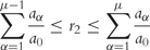
(5) The corresponding reaction Rμ is realized, i.e. the number of the participating molecules is increased or decreased according to the stoichiometry, and the time is incremented by τ. The whole process (1–4) is repeated as many times as necessary to reach the desired simulation time.
First Reaction Method
The First Reaction Method [5, 52] uses M random numbers in each step to compute putative reaction times τμ for each of the M reactions Rμ in the system. The τμ are exponentially distributed with parameter aμ. The reaction with the smallest reaction time τmin = min(τ1,…,τM), is executed and all putative reaction times are recalculated before the next step. Because of the wasteful use of random numbers and redundant recalculations the First Reaction Method is computationally inefficient. However, it can be numerically advantageous because, due to the machine-dependent resolution of floating-point numbers, the Direct Method cannot calculate rare reaction events amongst very frequent reactions in the system.
Next Reaction Method
Gibson and Bruck [54] improved the computational complexity of the First Reaction Method by the intelligent use of data structures:
A so-called dependency graph stores dependencies between the reactions → redundant recalculations of aμ are avoided.
Absolute putative reaction times τμ (since the beginning of simulation) are used instead of relative ones (since the last reaction event). Random numbers are ‘recycled’ during a reaction time update according to
 .
.An indexed priority queue contains all reactions sorted according to their putative reaction times → the next reaction can always be found in the root of the tree in constant time.
In the Next Reaction Method recalculations of aμ are minimized, and, asymptotically, only one random number per step is needed. Therefore it performs well, in particular, in the case of many reacting species and reactions.
Variants and extensions of the exact methods
Cao et al. (Optimized Direct Method [55]) and McCollum et al. (Sorting Direct Method [56]) reduce the computational cost of the Direct Method by sorting the reactions according to their propensities.
Li and Petzold (Logarithmic Direct Method [57]) use partial sums of propensities and a binary search for the next reaction in order to accelerate the computation.
Slepoy et al. [58] describe an algorithm that, in each iteration, chooses the next reaction event in constant-time independent of the number of different reactions.
The Direct Method has also been extended to accommodate delayed reactions often used to model, e.g. transcription or translocation processes [59–62].
Finally, there exist fast implementations that utilize special hardware, such as field-programmable gate arrays (FPGA) [63, 64] or computer clusters [65].
APPROXIMATE STOCHASTIC METHODS
The huge computational effort needed for exact stochastic simulation entailed a lively search for approximate simulation methods that sacrifice an acceptable amount of accuracy in order to speed up the simulation. The proposed methods often involve a grouping of reaction events (Probability-weighted Dynamic Monte Carlo (PW-DMC), τ-Leap Method), i.e. they permit more than one reaction event per step.
One approximate stochastic method, StochSim, does not primarily aim at speeding up the simulation and shall be discussed first.
StochSim, mesoscopic approach
In the mesoscopic approach by Morton-Firth (now Firth) [66–68] single particles are distinguished and represented by separate software objects. Though, their positions and velocities in the reaction volume are disregarded. This characteristic makes StochSim mesoscopic, residing on a middle conceptual level between microscopic molecular dynamics and macroscopic population-based approaches.
In each step two particles (or one particle and one pseudoparticle for monomolecular reactions) are randomly chosen. Whether a reaction event takes place between the two, is then determined using a random number and a look-up table.
This procedure can be even more time-consuming than the Direct Method when many nonreactive selections are chosen. The advantages are that multistate particles are possible (with different reaction rates for each configuration) and that the life-cycle of single particles can be traced. However, this could also be accomplished by extending one of the exact algorithms to keep track of single molecules.
The approach has also been extended to cover simple 2D-spatial modeling with stationary particles [69].
Probability-Weighted Dynamic Monte Carlo
The PW-DMC [70] (PW-DMC method) is a rather ad hoc approach in which reactions with high probability are allowed to fire multiple times. Instead of considering single fast reaction events separately, several events are grouped together and simulated as if they were one event. This reduces the effective propensity aμ of fast reactions and can reduce computation times, but has the major drawback that fluctuations can be misdescribed.
τ-Leap Methods
In 2001, Gillespie [71] developed an approximate stochastic simulation method named τ-Leap Method to accelerate the simulation procedure. This method avoids the meticulous reconstruction of every individual reaction event. Instead, it leaps along the time axis in steps of length τ containing many single reaction events. τ has to fulfill the so-called Leap Condition: it must be small enough that no significant change in the propensities aμ during [t,t+τ] occurs. Then, the reaction channels effectively decouple and the number of firings Kμ during time τ, starting from state x at time t, can be approximated by Poisson distributed random variables:
| (6) |
with 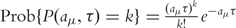 .
.
In each step a Poisson random number kμ is drawn for each reaction Rμ and the system state is updated according to:
| (7) |
Due to the drawing of Poisson random numbers, each τ-leap is more expensive than one step of the Direct or First Reaction Method. However, since many single reaction events can be leaped over when τ is large enough, the simulation can be much faster after all. Figure 1 illustrates the procedure.
Figure 1:

Schema of the τ-Leap Method.
The most important question remaining is how to choose an appropriate τ-value. Determining this value involves a trade-off between accuracy of the simulation and computation time. In the original article, Gillespie proposed a simple τ-choosing strategy. This has been improved upon in [72] and [73].
A number of variants and extensions of τ-Leaping have been developed recently that tackle some of the issues of the τ-Leap Method from 2001:
Rathinam et al. [74] draw on the analogy to numerical integration of ODEs and describe an ‘Implicit τ-Leaping Method’ in order to deal with stiffness in the system. This method has been improved by Cao and Petzold in [75]. The algorithm in [76] automatically switches between explicit and implicit τ-Leaping.
Tian and Burrage [77] and Chatterjee et al. [78] suggested to use (bounded) binomial random numbers instead of Poisson distributed ones. This so-called ‘Binomial τ-Leaping’ avoids one of the problems of the τ-Leap Method, namely the generation of negative particle numbers in some cases. An extension is the ‘Multinomial τ-Leaping Method’ in [79].
An alternative approach to avoid negative particle numbers has been developed by Cao et al. [80]. In this ‘Modified τ-Leaping Method’ exact stochastic simulation, allowing only one reaction event per step, is used for particle numbers that are critically low.
Burrage and Tian [81] constructed ‘Poisson Runge-Kutta Methods (PRK)’ to increase the efficiency of τ-Leaping.
The ‘R-Leaping’ in [82] and the ‘K-Leap Method’ in [83] are variants of the kα-Leaping method described in [71].
The ‘Unbiased τ-Leap Method’ [84] attempts to correct for the bias in τ-Leaping.
‘Binomial τ-DSSA’ [85] extends τ-Leaping by delayed reactions.
Finally, there is also a version for spatial simulations called ‘Bτ-SSSA’ by Marquez-Lago et al. 2007 [86].
Langevin Method
If the value of τ can be chosen big enough such that every reaction channel on average produces a very large number of firings ( ) while still satisfying the Leap Condition, the Poisson random variables can be approximated by normal random variables Nμ [87]:
| (8) |
| (9) |
In this case, the τ value is called to be ‘macroscopically infinitesimal’. The Poisson random variables for the system state update can be replaced by normal random variables which are easier to calculate. Conceptually, the procedure is now equivalent to the (chemical) Langevin equation, a stochastic differential equation (SDE):
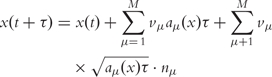 |
(10) |
with nμ unit normal random variables.
In the limiting case aμ(x)τ → ∞, the last (noise) term becomes negligibly small compared with the second (see [87]) yielding the Euler update method for the numerical integration of ODEs. The Langevin Method therefore illustrates how the SSA are connected to the deterministic method through a series of approximations (SSA → τ-Leap Method → Langevin Method → deterministic reaction rate equations).
Complex stochastic kinetics
The stochastic formalism is based on irreversible elementary reactions.
How to correctly handle derived kinetics, where a number of elementary reactions have been lumped into one complex reaction, is an important question because they are used in many models and often kinetic parameters for the underlying elementary reactions are not even known.
Bundschuh et al. 2003 [88] observed that a naive direct stochastic simulation of higher order kinetics can lead to a failure of correctly describing the fluctuations and even the mean of particle numbers. Nevertheless, in many cases the use of higher order terms in stochastic simulation is indeed justified as is discussed in Rao and Arkin [89] and Cao et al. [90] for the stochastic quasi-steady-state approximation (QSSA) and Michaelis–Menten kinetics (see also the Stochastic quasi-equilibrium approximations section below).
Hybrid methods
The basic idea of hybrid simulation methods is to combine the advantages of complementary simulation approaches: the whole system is subdivided into appropriate parts and different simulation methods operate on these parts at the same time. Figure 2 shows an exemplary schematic view of this procedure. Here, we have two subsystems containing the fast and slow reactions, respectively. Fast reactions often involve high-numbered species, e.g. in metabolism. Slow reactions or reactions involving low-numbered species can frequently be found in signal transduction or gene expression systems. The two subsystems are simulated iteratively by using adequate simulation methods, for instance, numerical integration of ODEs and stochastic simulation, respectively.
Figure 2:

Schematic view of an exemplary hybrid simulation method.
Mathematically, this corresponds to a partitioning of the CME (for a rigorous derivation of the partitioning process and mathematical details of the approximations employed, see [91–93]).
In between two reaction events in the slow/discrete subset of reactions, the fast subset evolves due to the action of the fast reactions only. This means that, during that time, its behavior can be approximated using ODEs, SDEs or approximate stochastic simulation methods independently of the slow subset.
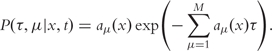
However, the reaction propensities aμ of slow reactions are, in general, also dependent on species whose concentrations are changed by fast reactions. Taking this into account, the slow subset no longer constitutes a homogeneous Poisson process. Instead, it has to be described by a Master Equation with time-varying transition propensities aμ(t). Gillespie [94] derives the correct Reaction Probability Density Function for this case:
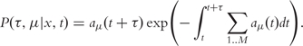 |
(11) |
Fast reactions involving high-numbered species (e.g. metabolism) can be simulated efficiently with hybrid algorithms. These reactions, in particular, would slow down a pure stochastic simulation considerably. This potential speed-up and that random fluctuations are considered where necessary are the main advantages of hybrid approaches.
Nevertheless, there are still some open questions:
Synchronization of the subnetworks? (Provision for time-varying aμ in the slow subnet. Conversion between continuous concentrations and discrete particle numbers.)
Reliable criteria for the partitioning?
How to handle fast reactions with small particle numbers involved?
Dynamic repartitioning → additional computational overhead.
For instance, dynamic/automated (re-)partitioning is not only important when the system state varies considerably over time, e.g. in oscillating systems. It also makes the methods much more user friendly by avoiding tedious modeler intervention. However, since dynamic partitioning causes computational overhead, the decision whether it should be used or not is always associated with a trade-off between user friendliness/accuracy and simulation speed. For very small systems it is probably not worthwhile to employ dynamic partitioning. A fixed partitioning can also be used when the subsystems are clearly different in terms of reaction velocities, for instance metabolic pathways coupled to signaling or reaction systems coupled by fast diffusion.
Likewise, on the one hand, taking into account time-varying aμ(t) in the slow/discrete subsystem requires algorithms that are mathematically more involved. On the other hand, the increase in accuracy associated with it renders additional updates of the propensities aμ(t) unnecessary so that larger steps can be taken.
Partitioning strategies based on reaction velocities usually aim at speeding up the simulation by taking the fast reactions out of the stochastically simulated subsystem. In contrast, particle number-based partitioning is more concerned with correctly treating reactions when particle numbers are so low that the system cannot be assumed continuous any longer. Usually a combination of different criteria are used for partitioning.
A number of hybrid algorithms [95–99] are based on a partitioning of the reaction system and the simulation of the slow subsystem using a stochastic algorithm which considers time-varying aμ, as described above. However, they differ in how exactly the nonhomogeneous Poisson process is sampled. Also, the partitioning strategies used are different, e.g. based on particle numbers, reaction velocities or (relative) level of fluctuations in particle numbers.
The hybrid methods in [91, 100, 101] also use a combination of stochastic simulation and numerical integration of ODEs/SDEs on a partitioned system, but do not consider time-varying aμ in the slow subsystem. Instead, for instance, the method by Haseltine and Rawlings [91] introduces a ‘probability of no reaction’ in order to limit the approximation error.
Other methods, e.g. combine the Next Reaction Method with τ-Leaping [102], employ agent-based frameworks [103] or meta-algorithms [104], use an implicit partitioning scheme [105], or integrate three [106] or even four [107] different methods into a hybrid simulation scheme.
Table 1 gives an overview of the different hybrid simulation methods. They are characterized along different dimensions, namely which methods they integrate, whether the partitioning is dynamic/automated or user-defined, which partitioning policy is used and whether or not time-varying aμ(t) in the slow/discrete subsystem(s) are considered or not (→ synchronization).
Table 1:
Overview and systematic classification of the different hybrid simulation methods
| Hybrid approaches | Methods combined | Dynamic partitioning | Partitioning criteria | Time-varying aμ |
|---|---|---|---|---|
| Alur et al. [103] | Direct Method/ODE | ✓ | Particle no. | |
| Haseltine and Rawlings [91] | Direct Method/ODE or SDE | Heuristics | ✓/× | |
| Pahle [100, 101] | Next Reaction Method/ODE | ✓ | Particle no. | |
| Adalsteinsson et al. [118] | Direct Method/ODE | User defined | ||
| Bentele and Eils [95] | Next Reaction Method/SDE | ✓ | Relat. fluct., particle no. | ✓ |
| Burrage et al. [106] | Direct M./τ-Leap/SDE | ✓ | Propensities, particle no. | |
| Kiehl et al. [120] | Direct Method/ODE | User defined | ✓/× | |
| Neogi et al. [96] | Stoch. Sim./ODE | ✓ | Particle no. | ✓ |
| Puchalka and Kierzek [102] | Next Reaction M./τ-Leap Method | ✓ | Substrate no., relat. prop. | |
| Takahashi et al. [104] | Next Reaction Method/ODE | User defined | ||
| Vasudeva and Bhalla [105] | Direct Method/ODE | ✓ | Propensities, particle no. | |
| Alfonsi et al. [97] | Next Reaction Method/SDE | ✓ | Propensities | ✓ |
| Salis and Kaznessis [121, 98] | Next Reaction Method/SDE | ✓ | Propensities, particle no. | ✓ |
| Griffith et al. [99] | Direct Method/ODE | ✓ | Propensities, particle no. | ✓ |
| Harris and Clancy [107] | Direct M./τ-Leap/Langevin M./ODE | ✓ | Propensities | |
| Wagner et al. [122] | First Reaction M./discr. Gauss/ODE | ✓ | Error criterion |
✓/× denotes that the authors describe how this feature can be realized in principle but do not demonstrate it in their examples or implementation.
Hybrid modeling and simulation might become particularly important in the future because of the emergence of ever more complex and heterogeneous models that integrate signaling, metabolism and gene expression and, as such, require a simulation on multiple scales.
Stochastic quasi-equilibrium approximation
Several authors proposed the use of quasi-equilibrium approximations (QEA) in stochastic simulations, e.g. [92, 93, 108–112].
For instance, Cao et al. [93] devised the ‘Slow-Scale Simulation Method’ in which the system is subdivided reaction- and species-wise into a fast and a slow subsystem. A ‘virtual fast process’ is defined which consists of the fast species evolving under only the fast reactions, i.e. all slow reactions are turned off. This process needs to be stable in a way such that its relaxation time is much faster than the expected time to the next slow reaction. Then, on the slow time scale, it can be approximated using its asymptotic solution. Finally, the system is simulated considering only the slow reaction events explicitly. For this, the Direct Method can be used with modified  (‘slow-scale propensity functions’). In each step, values for the fast species are determined by drawing random samples from the asymptotic probability distribution. Cao et al. give two simple examples for calculating the slow-scale propensities in their article, but this can be difficult for more complex models.
Stochastic QEA can be regarded as residing in the middle between exact stochastic simulation methods and hybrid approaches. The system is partitioned into subsets of reactions or species as in hybrid simulation methods. However, only the slow/discrete subset is explicitly simulated.
CONCLUSIONS
Stochastic modeling and simulation is important whenever fluctuation phenomena play a role either as a destructive or constructive element.
Despite of the multitude of proposed stochastic methods, there seems to be none that fits all problems. For smaller models in terms of particle numbers and whenever a correct treatment of the fluctuations is required, one of the exact methods should be used. There exist a number of corresponding software tools (Table 2), e.g. Copasi or Dizzy [113, 114] (see Table 2), and these methods are also relatively straightforward to implement.
Table 2:
List of selected software systems for biochemical systems capable of stochastic simulation
| Software | Methods | References |
|---|---|---|
| BioNetS | Direct Method, Langevin Eq., Hybrid Solver | [123, 118] |
| Cellware | Direct M., Next Reaction M., τ-Leap (explicit), Langevin-type Eq. with Poisson noise-term | [115, 124, 125] |
| Copasi | Next Reaction Method, Hybrid Solver | [113, 101] |
| Dizzy | Direct M., Next Reaction M., τ-Leap | [114, 126] |
| Dynetica | Direct Method | [127, 128] |
| E-Cell | Direct M., Next Reaction M., τ-Leap (implicit and explicit), Langevin Eq., Hybrid Solver | [116, 129] |
| Hy3S/SynBioSS | Direct M., Next Reaction M., SDE Solver, Hybrid Solver | [98, 110] |
| Jarnac | Direct Method | [130] |
| Kinetikit | Direct Method, Hybrid Solver | [131, 105] |
| MCell | Spatial stochastic simulation | [15, 16] |
| MesoRD | Spatial stochastic simulation | [17, 18, 19] |
| Moleculizer | First Reaction Method | [132, 133] |
| Smart Cell | Direct M., τ-Leap, Spatial stochastic simulation | [22, 23] |
| Smoldyn | Spatial stochastic simulation | [20, 21] |
| Stochastirator | Next Reaction Method | [134] |
| StochKit | Direct M., Optimized Direct M., Different τ-Leaping Methods, ssSSA, multiscale SSA | [117, 65] |
| StochSim | Stochastic mesoscopic approach | [135, 68, 67] |
| Stocks | Direct Method (lin. growing vol. & and cell division possible) | [136, 137] |
| Stode | Direct Method | [138, 139] |
The type of the simulation engines implemented and corresponding references are given.
For an accelerated stochastic simulation of bigger systems, one of the approximate methods could be considered. However, some of them are ad hoc procedures tailored to specific problems rather than general stochastic solvers. The particle-based StochSim algorithm might suit, if one wants to model multistate molecules or to trace the life-cycle of single particles. The τ-Leap Method or one of its variants seems to be a promising approach. However, this scheme is affected by stiffness which is often present in biochemical models. All approximate methods should be used with care. Their assumptions have to be thoroughly checked in each case. Otherwise they can misdescribe the fluctuations (e.g. the PW-DMC method and different forms of lumping) in some cases. With the exception of the τ-Leap Method (implemented in [22, 114–116] general software tools have been mostly missing. However, this has already started to change (see e.g. [117]). Some of the approximate methods are rather cumbersome to implement and they often need intervention by the modeler.
A very promising direction is the development of hybrid methods because they directly deal with the important problem of stiffness, which is often present in biochemical models. They appear to be flexible enough to allow for general stochastic solvers in the future even for very big and heterogeneous models. However, for the time being an established type of partitioning (reaction-wise and/or species-wise) and, above all, reliable criteria for an automatic and adaptive partitioning during the simulation are still missing. Hybrid algorithms are the most challenging methods to implement. Most of them also still need much user intervention. There exist already a few software tools, which allow for hybrid simulation, e.g. [65, 98, 101, 118], and this number is expected to grow in the future.
See Table 2 for a list of selected software systems which support stochastic simulation of biochemical systems. In addition, there is also the SBML stochastic test suite [119], which facilitates testing the accuracy of stochastic simulation software.
Key Points.
The dynamics of biochemical systems can be considerably affected by random fluctuations in discrete particle numbers.
Stochastic modeling and simulation are required to study these phenomena.
A multitude of different stochastic simulation methods have been proposed that can be classified as exact, approximate or hybrid.
Approximate methods have been developed to speed up the computationally expensive exact stochastic simulation.
Hybrid methods are particularly promising because they combine different approaches in order to deal with stiffness in biochemical models.
Acknowledgements
I would like to thank Ursula Kummer and Sven Sahle for many interesting discussions. Since the field has been growing considerably, in particular during the last few years, it is almost impossible to cover every method proposed. Therefore, my apologies to all authors whose work I did not cite in this article either due to space limitations or plain ignorance.
Biography
Jürgen Pahle is member of the ‘Modeling of Biological Processes’ group at the Bioquant, University of Heidelberg, Germany. His research focusses on stochastic simulation and analysis of biochemical networks.
References
- Endy D, Brent R. Modelling cellular behavior. Nature. 2001;409:391–5. doi: 10.1038/35053181. [DOI] [PubMed] [Google Scholar]
- Kitano H. Computational systems biology. Nature. 2002;420:206–10. doi: 10.1038/nature01254. [DOI] [PubMed] [Google Scholar]
- Heinrich R, Schuster S. The Regulation of Cellular Systems. New York, NY: Chapman and Hall; 1996. [Google Scholar]
- Hindmarsh AC. ODEPACK, a systematized collection of ODE solvers. In: Stepleman RS, Carver M, Peskin R, Ames WF, et al., editors. Scientific Computing, North-Holland, Amsterdam (Vol. 1 of IMACS Transactions on Scientific Computation) Amsterdam: North Holland; 1983. pp. 55–64. [Google Scholar]
- Gillespie DT. A general method for numerically simulating the stochastic time evolution of coupled chemical reactions. J Comput Phys. 1976;22:403–34. [Google Scholar]
- Kurtz TG. The relationship between stochastic and deterministic models for chemical reactions. J Chem Phys. 1972;57(7):2976–8. [Google Scholar]
- Kurtz TG. Strong approximation theorems for density dependent markov chains. Stoch Proc Appl. 1978;6(3):223–40. [Google Scholar]
- Turner TE, Schnell S, Burrage K. Stochastic approaches for modelling in vivo reactions. Comput Bio Chem. 2004;28:165–78. doi: 10.1016/j.compbiolchem.2004.05.001. [DOI] [PubMed] [Google Scholar]
- Meng TC, Somani S, Dhar P. Modeling and simulation of biological systems with stochasticity. In Silico Biol. 2004;4:0024. [PubMed] [Google Scholar]
- Gillespie DT. Stochastic simulation of chemical kinetics. Annu Rev Phys Chem. 2007;58:35–55. doi: 10.1146/annurev.physchem.58.032806.104637. [DOI] [PubMed] [Google Scholar]
- Lemerle C, Di Ventura B, Serrano L. Space as the final frontier in stochastic simulations of biological systems. FEBS Lett. 2005;579(8):1789–94. doi: 10.1016/j.febslet.2005.02.009. [DOI] [PubMed] [Google Scholar]
- Takahashi K, Arjunan SNV, Tomita M. Space in systems biology of signaling pathways – towards intracellular molecular crowding in silico. FEBS Lett. 2005;579(8):1783–8. doi: 10.1016/j.febslet.2005.01.072. [DOI] [PubMed] [Google Scholar]
- Tolle DP, Le Novère N. Particle-based stochastic simulation in systems biology. Curr Bioinform. 2006;1(3):315–20. [Google Scholar]
- Burrage K, Hancock J, Leier A, Nicolau DV., Jr Modelling and simulation techniques for membrane biology. Brief Bioinform. 2007;8(4):234–44. doi: 10.1093/bib/bbm033. [DOI] [PubMed] [Google Scholar]
- MCell. [(10 November 2008, date last accessed)]; http://www.mcell.cnl.salk.edu.
- Bartol TM, Jr, Land BR, Salpeter EE, Salpeter MM. Monte Carlo simulation of miniature endplate current generation in the vertebrate neuromuscular junction. Biophys J. 1991;59:1290–307. doi: 10.1016/S0006-3495(91)82344-X. [DOI] [PMC free article] [PubMed] [Google Scholar]
- MesoRD. [(10 November 2008, date last accessed)]; http://mesord.sourceforge.net.
- Hattne J, Fange D, Elf J. Stochastic reaction-diffusion simulation with MesoRD. Bioinformatics. 2005;21(12):2923–4. doi: 10.1093/bioinformatics/bti431. [DOI] [PubMed] [Google Scholar]
- Elf J, Ehrenberg M. Spontaneous separation of bi-stable chemical systems into spatial domains of opposite phases. Syst Biol. 2004;1(2):230–5. doi: 10.1049/sb:20045021. [DOI] [PubMed] [Google Scholar]
- Smoldyn. [(10 November 2008, date last accessed)]; http://www.smoldyn.org.
- Andrews SS, Bray D. Stochastic simulation of chemical reactions with spatial resolution and single molecule detail. Phys Biol. 2004;1(3):137–51. doi: 10.1088/1478-3967/1/3/001. [DOI] [PubMed] [Google Scholar]
- SmartCell. [(10 November 2008, date last accessed)]; http://smartcell.embl.de.
- Ander M, Beltrao P, Di Ventura B, et al. SmartCell, a framework to simulate cellular processes that combines stochastic approximation with diffusion and localisation: analysis of simple networks. IEE Syst Biol. 2004;1(1):129–38. doi: 10.1049/sb:20045017. [DOI] [PubMed] [Google Scholar]
- McAdams HH, Arkin A. It's a noisy business! Trends Genet. 1999;15(2):65–9. doi: 10.1016/s0168-9525(98)01659-x. [DOI] [PubMed] [Google Scholar]
- Arkin A, Ross J, McAdams HH. Stochastic kinetic analysis of developmental pathway bifurcation in phage λ-infected escherichia coli cells. Genetics. 1998;149:1633–48. doi: 10.1093/genetics/149.4.1633. [DOI] [PMC free article] [PubMed] [Google Scholar]
- Rao CV, Wolf DW, Arkin AP. Control, exploitation and tolerance of intracellular noise. Nature. 2002;420:231–7. doi: 10.1038/nature01258. [DOI] [PubMed] [Google Scholar]
- Érdi P, Tóth J. Mathematical Models of Chemical Reactions – Theory and Applications of Deterministic and Stochastic Models. Princeton, NJ: Princeton University Press; 1989. [Google Scholar]
- Qian H, Saffarin S, Elson EL. Concentration fluctuations in a mesoscopic oscillating chemical reaction system. Proc Natl Acad Sci USA. 2002;99(16):10376–81. doi: 10.1073/pnas.152007599. [DOI] [PMC free article] [PubMed] [Google Scholar]
- Samoilov M, Plyasunov S, Arkin AP. Stochastic amplification and signaling in enzymatic futile cycles through noise-induced bistability with oscillations. Proc Natl Acad Sci. 2005;102(7):2310–5. doi: 10.1073/pnas.0406841102. [DOI] [PMC free article] [PubMed] [Google Scholar]
- Kummer U, Krajnc B, Pahle J, et al. Transition from stochastic to deterministic behavior in calcium oscillations. Biophys J. 2005;89(3):1603–11. doi: 10.1529/biophysj.104.057216. [DOI] [PMC free article] [PubMed] [Google Scholar]
- Ross IL, Browne CM, Hume DA. Transcription of individual genes in eukaryotic cells occurs randomly and infrequently. Immunol Cell Biol. 1994;72(2):177–85. doi: 10.1038/icb.1994.26. [DOI] [PubMed] [Google Scholar]
- Barkai N, Leibler S. Circadian clocks limited by noise. Nature. 1999;403:267–8. doi: 10.1038/35002258. [DOI] [PubMed] [Google Scholar]
- Hallet MB. The unpredictability of cellular behavior: trivial or of fundamental importance to cell biology. Perspect Biol Med. 1999;33(1):110–9. doi: 10.1353/pbm.1990.0041. [DOI] [PubMed] [Google Scholar]
- Kuthan H. Self-organisation and orderly processes by individual protein complexes in the bacterial cell. Progr Biophys Mol Biol. 2001;75:1–17. doi: 10.1016/s0079-6107(00)00023-7. [DOI] [PubMed] [Google Scholar]
- Vilar JMG, Kueh HY, Barkai N, Leibler S. Mechanisms of noise-resistance in genetic oscillators. Proc Natl Acad Sci. 2002;99(9):5988–92. doi: 10.1073/pnas.092133899. [DOI] [PMC free article] [PubMed] [Google Scholar]
- Gunton JD, Toral R, Mirasso C, Gracheva ME. The role of noise in some physical and biological systems. Recent Res Devel Appl Phys. 2003;6:497. [Google Scholar]
- Gonze D, Halloy J, Goldbeter A. Emergence of coherent oscillations in stochastic models for circadian rhythms. Physica A. 2004;342:221–33. [Google Scholar]
- Kitano H. Biological robustness. Nat Rev Genet. 2004;5(11):826–37. doi: 10.1038/nrg1471. [DOI] [PubMed] [Google Scholar]
- Hume DA. Probability in transcriptional regulation and its implications for leukocyte differentiation and inducible gene expression. Blood. 2000;96(7):2323–8. [PubMed] [Google Scholar]
- Läer L, Kloppstech M, Schöfl C, et al. Noise enhanced hormonal signal transduction through intracellular calcium oscillations. Biophys Chem. 2001;91(2):157–66. doi: 10.1016/s0301-4622(01)00167-3. [DOI] [PubMed] [Google Scholar]
- Perc M, Marhl M. Noise enhances robustness of intracellular Ca2+ oscillations. Phys Lett A. 2003;316:304–10. [Google Scholar]
- Elowitz MB, Levine AJ, Siggia ED, Swain PS. Stochastic gene expression in a single cell. Science. 2002;297:1183–6. doi: 10.1126/science.1070919. [DOI] [PubMed] [Google Scholar]
- Ozbudak EM, Thattai M, Kurtser I, et al. Regulation of noise in the expression of a single gene. Nat Genet. 2002;31:69–73. doi: 10.1038/ng869. [DOI] [PubMed] [Google Scholar]
- Hallett MB, Pettit EJ. Stochastic events underlie Ca2+ signalling in neutrophils. J Theor Biol. 1997;186:1–6. doi: 10.1006/jtbi.1996.0345. [DOI] [PubMed] [Google Scholar]
- Kepler TB, Elston TC. Stochasticity in transcriptional regulation: origins, consequences, and mathematical representations. Biophys J. 2001;81:3116–36. doi: 10.1016/S0006-3495(01)75949-8. [DOI] [PMC free article] [PubMed] [Google Scholar]
- Wang L, Birol I, Hatzimanikatis V. Metabolic control analysis under uncertainty: Framework development and case studies. Biophys J. 2004;87:3750–63. doi: 10.1529/biophysj.104.048090. [DOI] [PMC free article] [PubMed] [Google Scholar]
- Gunawan R, Cao Y, Petzold L, Doyle FJ. Sensitivity analysis of discrete stochastic systems. Biophys J. 2005;88:2530–40. doi: 10.1529/biophysj.104.053405. [DOI] [PMC free article] [PubMed] [Google Scholar]
- McQuarrie DA. Stochastic approach to chemical kinetics. J Appl Prob. 1967;4(3):413–78. [Google Scholar]
- Laurenzi IJ. An analytical solution of the stochastic master equation for reversible bimolecular reaction kinetics. J Chem Phys. 2000;113(8):3315–22. [Google Scholar]
- Munsky B, Khammash M. The finite state projection algorithm for the solution of the chemical master equation. J Chem Phys. 2006;124:044104. doi: 10.1063/1.2145882. [DOI] [PubMed] [Google Scholar]
- MacNamara S, Burrage K, Sidje RB. Multiscale modeling of chemical kinetics via the master equation. Multiscale Model Simul. 2008;6(4):1146–68. [Google Scholar]
- Gillespie DT. Exact stochastic simulation of coupled chemical reactions. J Phys Chem. 1977;81(25):2340–61. [Google Scholar]
- Bortz AB, Kalos MH, Lebowitz JL. A new algorithm for monte carlo simulation of ising spin systems. J Comput Phys. 1975;17:10–18. [Google Scholar]
- Gibson MA, Bruck J. Efficient exact stochastic simulation of chemical systems with many species and many channels. J Phys Chem A. 2000;104(9):1876–89. [Google Scholar]
- Cao Y, Li H, Petzold L. Efficient formulation of the stochastic simulation algorithm for chemically reacting systems. J Chem Phys. 2004;121(9):4059–67. doi: 10.1063/1.1778376. [DOI] [PubMed] [Google Scholar]
- McCollum JM, Peterson GD, Cox CD, et al. The sorting direct method for stochastic simulation of bio-chemical systems with varying reaction execution behavior. Comput Biol Chem. 2006;30(1):39–49. doi: 10.1016/j.compbiolchem.2005.10.007. [DOI] [PubMed] [Google Scholar]
- Li H, Petzold L. Logarithmic direct method for discrete stochastic simulation of chemically reacting systems. [(10 November 2008, date last accessed)]; Technical Report. http://www.engr.ucsb.edu/~cse/
- Slepoy A, Thompson AP, Plimpton SJ. A constant-time kinetic Monte Carlo algorithm for simulation of large biochemical networks. J Chem Phys. 2008;128:205101. doi: 10.1063/1.2919546. [DOI] [PubMed] [Google Scholar]
- Bratsun D, Volfson D, Tsimring LS, Hasty J. Delay-induced stochastic oscillations in gene regulation. Proc Natl Acad Sci. 2005;102(41):14593–8. doi: 10.1073/pnas.0503858102. [DOI] [PMC free article] [PubMed] [Google Scholar]
- Barrio M, Burrage K, Leier A, Tian T. Oscillatory regulation of Hes1: discrete stochastic delay modelling and simulation. PLOS Comput Biol. 2006;2(9):e117. doi: 10.1371/journal.pcbi.0020117. [DOI] [PMC free article] [PubMed] [Google Scholar]
- Roussel MR, Zhu R. Validation of an algorithm for delay stochastic simulation of transcription and translation in prokaryotic gene expression. Phys Biol. 2006;3:274–84. doi: 10.1088/1478-3975/3/4/005. [DOI] [PubMed] [Google Scholar]
- Schlicht R, Winkler G. A delay stochastic process with applications in molecular biology. J Math Biol. 2008;57(5):613–48. doi: 10.1007/s00285-008-0178-y. [DOI] [PubMed] [Google Scholar]
- Salwinski L, Eisenberg D. In silico simulation of biological network dynamics. Nat Biotechnol. 2004;22:1017–9. doi: 10.1038/nbt991. [DOI] [PubMed] [Google Scholar]
- Osana Y, Fukushima T, Yoshimi M, et al. Proceedings of the 19th IEEE Int Par Distr Proc Symp. (IPDPS'05) Washington, DC, USA: IEEE Computer Society; 2005. An FPGA-based, multi-model simulation method for biochemical systems. In; p. 167.1. [Google Scholar]
- Li H, Cao H, Petzold LR, Gillespie DT. Algorithms and software for stochastic simulation of biochemical reacting systems. Biotechnol Prog. 2008;24:56–61. doi: 10.1021/bp070255h. [DOI] [PMC free article] [PubMed] [Google Scholar]
- Morton-Firth CJ. Stochastic Simulation of Cell Signaling Pathways. PhD thesis: University of Cambridge, UK; 1998. [Google Scholar]
- Morton-Firth CJ, Bray D. Predicting temporal fluctuations in an intracellular signalling pathway. J Theor Biol. 1998;192:117–28. doi: 10.1006/jtbi.1997.0651. [DOI] [PubMed] [Google Scholar]
- Le Novère N, Shimizu TS. StochSim: modelling of stochastic biomolecular processes. Bioinformatics. 2001;17(6):575–6. doi: 10.1093/bioinformatics/17.6.575. [DOI] [PubMed] [Google Scholar]
- Shimizu TS. Cell Signalling Pathways – A Computer-based Study. PhD thesis: University of Cambridge, UK; 2002. [Google Scholar]
- Resat H, Wiley HS, Dixon DA. Probability-weighted dynamic Monte Carlo method for reaction kinetics simulations. J Phys Chem B. 2001;105:11026–34. [Google Scholar]
- Gillespie DT. Approximate accelerated stochastic simulation of chemically reacting systems. J Chem Phys. 2001;115(4):1716–33. [Google Scholar]
- Gillespie DT, Petzold LR. Improved leap-size selection for accelerated stochastic simulation. J Chem Phys. 2003;119(16):8229–34. [Google Scholar]
- Cao Y, Gillespie DT, Petzold LR. Efficient step size selection for the tau-leaping simulation method. J Chem Phys. 2006;124:044109. doi: 10.1063/1.2159468. [DOI] [PubMed] [Google Scholar]
- Rathinam M, Petzold LR, Cao Y, Gillespie DT. Stiffness in stochastic chemically reacting systems: The implicit tau-leaping method. J Chem Phys. 2003;119(24):12784–94. [Google Scholar]
- Cao Y, Petzold L. Proceedings of Foundations of Systems Biology Engineering (FOSBE 2005) 2005. Trapezoidal tau-leaping formula for the stochastic simulation of biochemical systems; pp. 149–152. [Google Scholar]
- Cao Y, Gillespie DT, Petzold LR. Adaptive explicit-implicit tau-leaping method with automatic tau selection. J Chem Phys. 2007;126(22):224101. doi: 10.1063/1.2745299. [DOI] [PubMed] [Google Scholar]
- Tian T, Burrage K. Binomial leap methods for simulating stochastic chemical kinetics. J Chem Phys. 2004;121(21):10356–64. doi: 10.1063/1.1810475. [DOI] [PubMed] [Google Scholar]
- Chatterjee A, Vlachos DG, Katsoulakis MA. Binomial distribution based τ-leap accelerated stochastic simulation. J Chem Phys. 2005;122(2):024112. doi: 10.1063/1.1833357. [DOI] [PubMed] [Google Scholar]
- Pettigrew MF, Resat H. Multinomial tau-leaping method for stochastic kinetic simulations. J Chem Phys. 2007;126:084101. doi: 10.1063/1.2432326. [DOI] [PubMed] [Google Scholar]
- Cao Y, Gillespie DT, Petzold LR. Avoiding negative populations in explicit Poisson tau-leaping. J Chem Phys. 2005;123(5):054104. doi: 10.1063/1.1992473. [DOI] [PubMed] [Google Scholar]
- Burrage K, Tian T. Poisson Runge-Kutta methods for chemical reaction systems. In: Lu YY, Sun W, Tang T, editors. Advances in Scientific Computing and Applications – Third International Workshop on Scientific Computing and Applications. Beijing: Science Press; 2004. pp. 82–96. [Google Scholar]
- Auger A, Chatelain P, Koumoutsakos P. R-leaping: accelerating the stochastic simulation algorithm by reaction leaps. J Chem Phys. 2006;125(8):084103. doi: 10.1063/1.2218339. [DOI] [PubMed] [Google Scholar]
- Cai X, Xu Z. K-leap method for accelerating stochastic simulation of coupled chemical reactions. J Chem Phys. 2007;126:074102. doi: 10.1063/1.2436869. [DOI] [PubMed] [Google Scholar]
- Xu Z, Cai X. Unbiased τ-leap methods for stochastic simulation of chemically reacting systems. J Chem Phys. 2008;128:154112. doi: 10.1063/1.2894479. [DOI] [PubMed] [Google Scholar]
- Leier A, Marquez-Lago TT, Burrage K. Generalized binomial τ-leap method for biochemical kinetics incorporating both delay and intrinsic noise. J Chem Phys. 2008;128:205107. doi: 10.1063/1.2919124. [DOI] [PubMed] [Google Scholar]
- Marquez-Lago TT, Burrage K. Binomial tau-leap spatial stochastic simulation algorithm for applications in chemical kinetics. J Chem Phys. 2007;127:104101. doi: 10.1063/1.2771548. [DOI] [PubMed] [Google Scholar]
- Gillespie DT. The chemical Langevin equation. J Chem Phys. 2000;113(1):297–306. [Google Scholar]
- Bundschuh R, Hayot F, Jayaprakash C. Fluctuations and slow variables in genetic networks. Biophys J. 2003;84:1606–15. doi: 10.1016/S0006-3495(03)74970-4. [DOI] [PMC free article] [PubMed] [Google Scholar]
- Rao CV, Arkin AP. Stochastic chemical kinetics and the quasi-steady-state assumption: Application to the Gillespie algorithm. J Chem Phys. 2003;118(11):4999–5010. [Google Scholar]
- Cao Y, Gillespie DT, Petzold LR. Accelerated stochastic simulation of the stiff enzyme-substrate reaction. J Chem Phys. 2005;123:144917. doi: 10.1063/1.2052596. [DOI] [PubMed] [Google Scholar]
- Haseltine EL, Rawlings JB. Approximate simulation of coupled fast and slow reactions for stochastic chemical kinetics. J Chem Phys. 2002;117(15):6959–69. [Google Scholar]
- Haseltine EL, Rawlings JB. On the origins of approximations for the stochastic chemical kinetics. J Chem Phys. 2005;123:164115. doi: 10.1063/1.2062048. [DOI] [PubMed] [Google Scholar]
- Cao Y, Gillespie DT, Petzold LR. The slow-scale stochastic simulation algorithm. J Chem Phys. 2005;122(1):014116. doi: 10.1063/1.1824902. [DOI] [PubMed] [Google Scholar]
- Gillespie DT. Marcov Processes – An Introduction for Physical Scientists. San Diego, CA: Academic Press: Inc.; 1992. [Google Scholar]
- Bentele M, Eils R. Computational Methods in Systems Biology CMSB, LNCS. Heidelberg: Springer; 2004. General stochastic hybrid method for the simulation of chemical reaction processes in cells. In; pp. 248–51. [Google Scholar]
- Neogi NA. Hybrid Systems: Computation and Control, HSCC 2004, LNCS 2993. Heidelberg: Springer; 2004. Dynamic partitioning of large discrete event biological systems for hybrid simulation and analysis. In; pp. 463–476. [Google Scholar]
- Alfonsi A, Cancès E, Turinici G, et al. Adaptive simulation of hybrid stochastic and deterministic models for biochemical systems. In. ESAIM Proc. 2005;14:1–13. [Google Scholar]
- Salis H, Sotiropoulus V, Kaznessis YN. Multiscale Hy3S: Hybrid stochastic simulation for supercomputers. BMC Bioinform. 2006;7:93. doi: 10.1186/1471-2105-7-93. [DOI] [PMC free article] [PubMed] [Google Scholar]
- Griffith M, Courtney T, Peccoud J, Sanders WH. Dynamic partitioning for hybrid simulation of the bistable HIV-1 transactivation network. Bioinformatics. 2006;22(22):2782–9. doi: 10.1093/bioinformatics/btl465. [DOI] [PubMed] [Google Scholar]
- Pahle J. Eine Hybridmethode zur Simulation biochemischer Prozesse [in German] Heidelberg: ILKD, Universität Karlsruhe (TH) and EML; 2002. Diploma thesis. [Google Scholar]
- Hoops S, Sahle S, Gauges R, et al. COPASI – a COmplex PAthway SImulator. Bioinformatics. 2006;22(24):3067–74. doi: 10.1093/bioinformatics/btl485. [DOI] [PubMed] [Google Scholar]
- Puchalka J, Kierzek AM. Bridging the gap between stochastic and deterministic regimes in the kinetic simulations of the biochemical reaction networks. Biophys J. 2004;86(3):1357–72. doi: 10.1016/S0006-3495(04)74207-1. [DOI] [PMC free article] [PubMed] [Google Scholar]
- Alur R, Belta C, Ivančić F, et al. Lecture Notes in Computer Science, Proceedings of the 4th International Workshop on Hybrid Systems: Computation and Control. Vol. 2034. Berlin/Heidelberg: Springer; 2001. Hybrid modeling and simulation of biomolecular networks; pp. 19–32. [Google Scholar]
- Takahashi K, Kaizu K, Hu B, Tomita M. A multi-algorithm, multi-timescale method for cell simulation. Bioinformatics. 2004;20(4):538–546. doi: 10.1093/bioinformatics/btg442. [DOI] [PubMed] [Google Scholar]
- Vasudeva K, Bhalla US. Adaptive stochastic-deterministic chemical kinetic simulations. Bioinformatics. 2004;20(1):78–84. doi: 10.1093/bioinformatics/btg376. [DOI] [PubMed] [Google Scholar]
- Burrage K, Tian T, Burrage P. A multi-scaled approach for simulating chemical reaction systems. Prog Biophys Mol Biol. 2004;85:217–34. doi: 10.1016/j.pbiomolbio.2004.01.014. [DOI] [PubMed] [Google Scholar]
- Harris LA, Clancy P. A ‘partitioned leaping’ approach for multiscale modeling of chemical reaction dynamics. J Chem Phys. 2006;125:144107. doi: 10.1063/1.2354085. [DOI] [PubMed] [Google Scholar]
- Cao Y, Gillespie D, Petzold L. Multiscale stochastic simulation algorithm with stochastic partial equlibrium assumption for chemically reacting systems. J Comput Phys. 2005;206(2):395–411. [Google Scholar]
- E W, Liu D, Vanden-Eijnden E. Nested stochastic simulation algorithm for chemical kinetic systems with disparate rates. J Chem Phys. 2005;123:194107. doi: 10.1063/1.2109987. [DOI] [PubMed] [Google Scholar]
- Salis H, Kaznessis YN. An equation-free probabilistic steady-state approximation: dynamic application to the stochastic simulation of biochemical reaction networks. J Chem Phys. 2005;123:214106. doi: 10.1063/1.2131050. [DOI] [PubMed] [Google Scholar]
- Goutsias J. Quasiequilibrium approximation of fast reaction kinetics in stochastic biochemical systems. J Chem Phys. 2005;122:184102. doi: 10.1063/1.1889434. [DOI] [PubMed] [Google Scholar]
- Samant A, Vlachos DG. Overcoming stiffness from stochastic simulation stemming from partial equilibrium: a multiscale Monte Carlo algorithm. J Chem Phys. 2005;123(14):144114. doi: 10.1063/1.2046628. [DOI] [PubMed] [Google Scholar]
- Copasi. [(10 November 2008, date last accessed)]; http://www.copasi.org.
- Dizzy. [(10 November 2008, date last accessed)]; http://magnet.systemsbiology.net/software/Dizzy.
- Cellware. [(10 November 2008, date last accessed)]; http://www.cellware.org.
- E-Cell. [(10 November 2008, date last accessed)]; http://www.e-cell.org.
- StochKit. [(10 November 2008, date last accessed)]; http://www.engr.ucsb.edu/~cse.
- Adalsteinsson D, McMillen D, Elston TC. Biochemical network stochastic simulator (BioNetS): software for stochastic modeling of biochemical networks. BMC Bioinform. 2004;5(1):24. doi: 10.1186/1471-2105-5-24. [DOI] [PMC free article] [PubMed] [Google Scholar]
- Evans TW, Gillespie CS, Wilkinson DJ. The SBML discrete stochastic models test suite. Bioinformatics. 2008;24(2):285–6. doi: 10.1093/bioinformatics/btm566. [DOI] [PubMed] [Google Scholar]
- Kiehl TR, Mattheyses RM, Simmons MK. Hybrid simulation of cellular behavior. Bioinformatics. 2004;20(3):316–22. doi: 10.1093/bioinformatics/btg409. [DOI] [PubMed] [Google Scholar]
- Salis H, Kaznessis Y. Accurate hybrid stochastic simulation of a system of coupled chemical or biochemical reactions. J Chem Phys. 2005;122(5):054103. doi: 10.1063/1.1835951. [DOI] [PubMed] [Google Scholar]
- Wagner H, Möller M, Prank K. COAST: Controllable approximative stochastic reaction algorithm. J Chem Phys. 2006;125(17):174104. doi: 10.1063/1.2361284. [DOI] [PubMed] [Google Scholar]
- BioNetS. [(10 November 2008, date last accessed)]; http://x.amath.unc.edu/BioNetS.
- Dhar P, Meng TC, Somani S, et al. Cellware – a multi-algorithmic software for computational systems biology. Bioinformatics. 2004;20(8):1319–21. doi: 10.1093/bioinformatics/bth067. [DOI] [PubMed] [Google Scholar]
- Dhar PK, Meng TC, Somani S, et al. Grid cellware: the first grid-enabled tool for modelling and simulating the cellular processes. Bioinformatics. 2005;21(7):1284–7. doi: 10.1093/bioinformatics/bti143. [DOI] [PubMed] [Google Scholar]
- Ramsey S, Orrell D, Bolouri H. Dizzy: stochastic simulation of large-scale genetic regulatory networks. J Bioinform Comput Biol. 2005;3(2):415–36. doi: 10.1142/s0219720005001132. [DOI] [PubMed] [Google Scholar]
- Dynetica. [(10 November 2008, date last accessed)]; http://www.duke.edu/~you/Dynetica_page.htm.
- You L, Hoonlor A, Yin J. Modeling biological systems using Dynetica – a simulator of dynamic networks. Bioinformatics. 2003;19(3):435–6. doi: 10.1093/bioinformatics/btg009. [DOI] [PubMed] [Google Scholar]
- Tomita M, Hashimoto K, Takahashi K, et al. E-CELL: software environment for whole-cell simulation. Bioinformatics. 1999;15(1):72–84. doi: 10.1093/bioinformatics/15.1.72. [DOI] [PubMed] [Google Scholar]
- Jarnac. [(10 November 2008, date last accessed)]; http://sys-bio.org/software/jarnac.htm.
- Kinetikit. [(10 November 2008, date last accessed)]; http://www.ncbs.res.in/
- Moleculizer. [(10 November 2008, date last accessed)]; http://www.molsci.org/~lok/moleculizer.
- Lok L, Brent R. Automatic generation of cellular reaction networks with Moleculizer 1.0. Nat Biotechnol. 2005;23(1):131–6. doi: 10.1038/nbt1054. [DOI] [PubMed] [Google Scholar]
- Stochastirator. [(10 November 2008, date last accessed)]; http://openwetware.org/wiki/Endy:Software.
- StochSim. [(10 November 2008, date last accessed)]; http://www.pdn.cam.ac.uk/groups/comp-cell/StochSim.html.
- Stocks. [(10 November 2008, date last accessed)]; http://www.ibb.waw.pl/stocks.
- Kierzek AM. STOCKS: STOChastic Kinetic Simulations of biochemical systems with Gillespie algorithm. Bioinformatics. 2002;18(3):470–81. doi: 10.1093/bioinformatics/18.3.470. [DOI] [PubMed] [Google Scholar]
- Stode. [(10 November 2008, date last accessed)]; http://projects.villa-bosch.de/bcb/software/Carel.
- van Gend C, Kummer U. STODE – automatic stochastic simulation of systems described by differential equations. In: Yi T-M, Hucka M, Morohashi M, Kitano H, editors. 2001. pp. 326–33. Proceedings of the Second International Conference on Systems Biology ICSB. [Google Scholar]