Sparse combinatorial inference with an application in cancer biology

Abstract

Motivation: Combinatorial effects, in which several variables jointly influence an output or response, play an important role in biological systems. In many settings, Boolean functions provide a natural way to describe such influences. However, biochemical data using which we may wish to characterize such influences are usually subject to much variability. Furthermore, in high-throughput biological settings Boolean relationships of interest are very often sparse, in the sense of being embedded in an overall dataset of higher dimensionality. This motivates a need for statistical methods capable of making inferences regarding Boolean functions under conditions of noise and sparsity.

Results: We put forward a statistical model for sparse, noisy Boolean functions and methods for inference under the model. We focus on the case in which the form of the underlying Boolean function, as well as the number and identity of its inputs are all unknown. We present results on synthetic data and on a study of signalling proteins in cancer biology.

Availability: go.warwick.ac.uk/sachmukherjee/sci

Contact: s.n.mukherjee@warwick.ac.uk

1 INTRODUCTION

Recent years have witnessed a growing trend towards thinking about multiple biological components or players acting in concert, rather than one at a time. Biological systems are rich with examples of combinatorial regulation and influence. At the molecular level, in systems such as protein signalling pathways or gene regulatory networks, several components may jointly influence the state of a downstream target. Equally, at the level of cellular or tissue-level outcomes, complex interplay involving underlying molecular components (such as feedback and inhibition) may induce a combinatorial relationship between the state of such components and an indicator of interest, such as drug sensitivity or disease status. Finally, at the population level, multiple genetic features, such as haplotypes, may jointly influence phenotypic status.

In many settings in which data are either binary or amenable to binary transformation, the language of Boolean logic provides a natural way to describe combinatorial influences. That is, we can think of a binary output or response Y as a k-ary Boolean function of binary arguments X₁ ··· X_k. In this article, we address the question of making inferences regarding Boolean models of combinatorial influence. In the context of high-throughput biology this is challenging for two key reasons. First, Boolean functions are inherently non-linear. This means that the importance of a set of variables taken together may not be reflected in the importance of the same variables considered one at a time. Second, in system-wide assays, the inputs to an underlying Boolean relationship of interest may be embedded in an overall dataset of much higher dimensionality. Returning to the protein signalling example alluded to above, a Boolean relationship between the activation states of a pair of cytosolic kinases and a downstream effect may be embedded in a dataset pertaining to dozens of other pathway components.

Motivated by these issues, in this article we place an emphasis on sparse Boolean functions. An emphasis on sparsity plays a key role in rendering inference tractable, in both computational and statistical terms. The size of the space of possible Boolean functions is vast: for p predictors there are 2^p possible subsets of variables, and for any variable subset of size k, 2^k possible states of k binary arguments, and therefore 2^2k possible Boolean functions of those arguments. Equally, from the statistical point of view, parsimonious models can be highly advantageous, especially under conditions of small-to-moderate sample size. Furthermore, from the point of view of performing follow-up work, sparse models are helpful because they focus attention on a small number of players, which in turn can help to suggest specific experimental strategies.

Characterizing sparse Boolean functions from noisy data involves addressing two related problems. First, we must determine which of a possibly large number of predictors are arguments to the underlying function; this involves selecting a subset (of unknown size) of available predictors. Second, for a putative set of k arguments, we must say something about possible k-ary Boolean functions. Motivated by real-world problems in statistical bioinformatics, we focus on the setting in which both arity k and the specific subset of predictors which are arguments to the underlying Boolean function are unknown: i.e. we know neither how many variables are important nor which ones they are. We propose a simple probability model for Boolean functions that are subject to stochastic variation in observed data. We then use ideas from Bayesian inference to build on the probability model and learn Boolean relationships from noisy data, using prior distributions to take advantage of a notion of sparsity. A key advantage of our statistical approach is that it allows us to account for variability in data, and also to provide a measure of confidence in any inferences drawn. This latter point is especially important when follow-up investigations are costly or time-consuming. Furthermore, as discussed below, our methods require typically no more than a few minutes of computer time.

Our focus is on making inferences regarding sparse, noisy Boolean functions rather than classification per se. However, since the range of a Boolean function is {0, 1}, the task of predicting a response value Y from predictors X is analogous to a classification problem. Our work is similar in spirit to logic regression (Kooperberg and Ruczinski, 2005; Ruczinski et al., 2003); we contrast the two in Section 5 (Discussion) below. Other related work on noisy Boolean functions includes Benjamini et al. (1999), Shmulevich et al. (2002) and Li and Lu (2005).

The remainder of this article is organized as follows. We first introduce the key elements of our model and associated notation, and then discuss inference. We present experimental results on synthetic data and on a proteomic dataset from a study in cancer systems biology. Finally, we discuss some of the finer points and shortcomings of our work and highlight key directions for further research.

2 BASIC MODEL AND NOTATION

2.1 Noisy Boolean functions

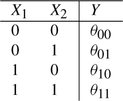
A k-ary Boolean function is a function f: {0,1}^k ↦ {0,1} which maps each of the 2^k possible states of its binary arguments X = (X₁ ··· X_k) to a binary state Y. Such a function can also be represented as a truth table.

Now, consider a function g_θ: {0,1}^k ↦ [0,1], that maps each of the ^k possible states of its arguments to the (closed) unit interval. In particular, when inputs X are in state x, g_θ returns a value θ_x= g_θ(x) that represents the probability with which the output Y takes on value 1. For the moment, we do not place any restrictions on the θ_x's, but we return to these parameters in the context of inference below. We call the function g_θ a noisy Boolean function. A noisy Boolean function can be represented by a probabilistic truth table:

A conventional truth table can then be regarded as a special, ‘noise free’ case of a probabilistic truth table, with parameters θ_x equal to 0 or 1. It is natural to assume that if a Boolean function evaluates true for a given state x of its inputs, the response for a ‘noisy version’ of the function should be true more often than false. Accordingly, if for all x, 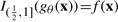(where I_A is the indicator function for set A), we say that g_θ corresponds to Boolean function f. We can then construct a Boolean function f from a noisy Boolean function g_θ by the following rule:

(1)

This defines a (many-to-one) mapping between the space of noisy Boolean functions and the space of Boolean functions; we call this mapping Ψ and write f = Ψ(g_θ).

2.2 Probability model

Let Y = (Y₁ … Y_n), Y_i ∈ {0, 1} denote binary responses and X = (X₁ … X_n), X_i ∈ {0, 1}^d corresponding d-dimensional predictors. We denote the i-th observation of the j-th predictor by X_ij, the i-th observation of predictors A ⊆ {1 … d} by X_iA and the full set of n observations of predictors A by X_{· A} = (X_{1 A} … X_{n A}).

Suppose Y is a noisy Boolean function of a subset M ⊆ {1 … d} of predictors. The specification of this subset represents a model; for notational simplicity, we will use M to denote both the subset and the model it implies. We assume that, under model M, an observation Y_i is conditionally independent of all other predictors given X_iM:

(2)

Suppose the relevant predictors X_iM are in state x. Then, θ_x = g_θ(x) is the corresponding parameter in the probabilistic truth table, and represents the probability of the event Y_i=1 given the state of the predictors. In other words, Y_i | X_iM=x is a Bernoulli random variable with success parameter θ_x. We assume that, given the state of predictors X_iM, Y₁ … Y_n are independent and identically distributed. Then the joint probability of the Y_i's, given X_·M, is a product of Binomial kernels:

(3)

where θ is a parameter vector with components θ_x, n_B = ∑_i: X_iM = x 1 is the number of observations in which predictors X_·M are in state x and ν_x = ∑_i: X_iM = x Y_i is the corresponding number of ‘successes’ of Y_i when X_·M=x.

3 INFERENCE

In this section, we discuss model selection, parameter estimation and prediction using the model introduced above.

3.1 Model selection

Each model corresponds to a subset M ⊆ {1 … d} of predictors. As such, there are, unconstrained, 2^d distinct models. Restricting attention to sparse Boolean functions with maximum arity k_max, the number of possible models is 𝒪(d^k_max). The sheer size of model space—even under conditions of sparsity—makes model selection a central concern in inference regarding Boolean functions. Furthermore, since noisy Boolean functions can give rise to responses which depend on non-linear interplay between predictors, variable selection using marginal statistics will not, in general, be able to capture the joint explanatory power of a subset of predictors. In contrast, the state-dependent model introduced above allows us to consider all ‘Boolean’ interactions between arguments. In this section, we exploit our probability model to develop a Bayesian approach to model selection in this setting, using Markov chain Monte Carlo (MCMC) to draw samples from the posterior distribution over models.

3.1.1 Model posterior

From Bayes' rule, the posterior probability of a model M can be written up to proportionality as:

(4)

The term P(Y | X_·M) represents the marginal likelihood. This can be obtained by integrating out parameters θ:

(5)

Let Θ represent the full parameter space, such that θ ∈ Θ. Now, for any Boolean function f, there exists some subset of Θ which maps to f under mapping (1). Integrating out θ therefore corresponds to averaging over all possible Boolean functions with arguments M.

3.1.2 Parameter prior

We first assume prior independence of parameters θ_x, such that p(θ) = ∏_xp(θ_x). Then, from (3) and (5), we get:

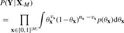(6)

In light of the relationship between parameters θ_x and underlying Boolean functions, there are two properties we would like the parameter prior p(θ_x) to have. First, given a model M corresponding to a Boolean function of arity k = |M|, we would like to assign equal probability to all Boolean functions possible under the model. Second, since the parameters θ_x represent state-dependent success parameters for a noisy Boolean function, we would like the prior to prefer values close to 0 or 1. Now, for any continuous prior density symmetric about , 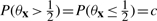(say). 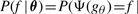From mapping (1), the probability of a k-ary Boolean function f, given k independent parameters θ_x is: , which is constant over the space of k-ary Boolean functions. Thus, under prior parameter independence, symmetry about ensures the first of our two desiderata.

We therefore suggest a Beta prior p(θ_x) with identical parameters α, β (for symmetry) and α, β > 1 (to concentrate probability mass around 0 and 1). This gives the marginal likelihood (6) in closed form:

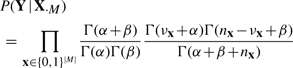(7)

In all our experiments, we set α,β=0.9.

3.1.3 Sparse model prior

We use the model prior P(M) to express an explicit preference for sparse models. We suggest the following prior:

(8)

where hyper-parameter k₀ is a threshold on subset size |M|, below which the prior is flat, and λ is a strength parameter. In all our experiments, we set λ=3. Hyper-parameter k_max allows us to set a hard upper limit on model size, if desired (otherwise, k_max should be set to p).

A natural way to set hyper-parameters k₀ and k_max is as a function of sample size. For |M| ≤ k₀, the prior is agnostic to model size. The expected number of observations per input state is therefore n/2^k₀ for the largest model inferred without reference to the sparsity prior. If we desire at least n* observations per state in this boundary case, this gives k₀=⌊ log₂ (n/n*) ⌋. In all our experiments we set k₀ in this way with n*=15. We set k_max in a similar manner, with n*=1, giving k_max=⌊ log₂ (n) ⌋. This ensures that we only consider models sparse enough to have, on average, at least one observation per input state.

3.1.4 Markov chain Monte Carlo

The space of all possible models is, in general, too large to permit a full description of the posterior Equation (4). This motivates the need for approximate inference. Here, we propose a MCMC sampler over model space.

In our approach, a model is equivalent to a subset M of predictor indices {1 … d}. Let ℐ(M) be a set comprising all subsets which can be obtained by either adding exactly one element to the set M, or by removing exactly one element from it. That is,

(9)

We suggest the following proposal distribution Q:

(10)

where, M and M′ denote current and proposed models, respectively.

Importantly, during sampling, the unnormalized quantities P(Y | X_·M′) P(M′) and P(Y | X_·M) P(M), which can be obtained in closed-form from (7) and (8), are sufficient for our purposes. Note also that since any subset of {1 … d} can be reached from an arbitrary starting subset by some sequence of addition and removal steps, the proposal distribution Q gives rise to an irreducible Markov chain. Standard results (Robert and Casella, 2004) then guarantee convergence to the desired posterior P(M | Y, X). The sampler described above is summarized in Algorithm 1.

Algorithm 1.

Metropolis-Hastings sampler for model selection

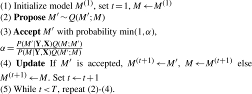As shown in Algorithm 1, iterating ‘propose’, ‘accept’ and ‘update’ steps gives rise to T samples M⁽¹⁾ … M^(T). An important property of these samples is that, provided the Markov chain has converged, is an asymptotically valid estimator of the expectation, under the posterior, of a function ϕ(M).

An important special case, which we shall make use of below, concerns the posterior probability P(j ∈ M | Y, X) that a variable j ∈ {1 … d} is part of the underlying model M. This is equivalent to the posterior expectation 𝔼[I_M(j)]_{P(M | Y, X)}, which in turn gives

(11)

as an asymptotically valid estimate of P(j ∈ M | Y, X).

Standard MCMC diagnostics using multiple chains with different initializations showed rapid convergence. Posterior probabilities over individual predictors, computed using Equation (11), were very consistent across diagnostic runs, giving us confidence that probabilities obtained were not simply artefacts of poor convergence.

Finally, we note that an alternative to sampling from the posterior over models is to estimate a single, maximum a posteriori model :

(12)

This can be done using, for example, greedy local optimization in model space, with multiple, random initializations to guard against local maxima.

3.2 Parameter estimation and prediction

From standard Bayesian results (Gelman et al., 2004), the posterior distribution of parameter θ_x is easily shown to be:

(13)

Similarly, the posterior probability that a new, unseen response Y(n+1) will take on the value 1, given that predictors X_(n+1)M are observed in state x is obtained as follows. Let X_·M = X_1M … X_nM and Y = Y₁ … Y_n denote already observed data. Then, using Equation (13) we get:

(14)

4 RESULTS

In this section, we present empirical results examining the ability of our methods to make inferences regarding sparse Boolean functions. We first show results from synthetic datasets and then present an analysis of proteomic data pertaining to subtypes of breast cancer.

4.1 Synthetic data

We generated 10 datasets from each of three different sparse Boolean models. Denoting the elements of the relevant subset as A, B, C, etc., we considered three models M1, M2 and M3 based on the following Boolean functions:

• (M1) A ∧ (B ⇔ C)

• (M2) (A ∧ ¬ B)XORC

• (M3) (A ∧ B)XOR(C ∧ D)

In each case, the relevant predictors formed a subset of a total of d=100 variables. Data were generated in the following manner: (i) for i=1 … n(n=200) and j=1 … d(d=100), we set X_ij at random and then generated responses by setting Y_i=1 with probability 0.9 when f(A, B, …) evaluated true (and zero otherwise) and setting Y_i=1 with probability 0.1 when ¬ f (and zero otherwise). In other words, the data-generating model was a noisy Boolean function with underlying Boolean function f and parameters θ_x=0.9 and θ_x=0.1 for f(x)=1 and f(x)=0, respectively. The sample size n=200 led us to automatically set sparsity hyper-parameters k₀=⌊log₂n/n*⌋ = 3 and k_max=⌊log₂n⌋=7 (this gives on the order of 10¹⁰ possible models of arity not exceeding k_max=7). We used MCMC as described above, with T = 10 000 samples drawn for each analysis, and 1000 samples discarded as ‘burn-in’.

Figure 1a–c shows, for each model, Receiver Operating Characteristic (ROC) curves obtained by thresholding posterior probabilities over individual predictors, following Equation (11). For comparison we also show corresponding results obtained using (absolute) log odds ratios and Fisher scores. The log odds ratio is a natural measure of pairwise association for binary data (Edwards, 1963). Here we computed the log odds ratio between each predictor and the response. The Fisher score (Duda et al., 2000) is a simple and widely used variable selection approach; here, variables were ranked by the ratio between the squared difference between class means and the pooled standard deviation (classes corresponded to observations for which the response was 0 or 1). The ROC curves shown are averages over results obtained from the 10 datasets generated for each model.

Fig. 1.

Simulated data, ROC curves and posterior probabilities over predictors. (a–c) are ROC curves showing true positive rates in selecting relevant inputs plotted against corresponding false positive rates, across a range of thresholds. Results are also shown for Fisher scores and log odds ratios (computed between each predictor and the response. (d–f) show typical posterior probabilities over individual predictors; predictors which truly form part of the underlying model are plotted in green while other predictors are plotted in red.

Our approach is effective for each of the three models. In contrast, neither log odds ratios nor Fisher scores are able to discover the correct variables for any of the models. This is unsurprising, because these methods are based on marginal statistics, in effect scoring each predictor in isolation. As noted at the outset of the paper, an important characteristic of many Boolean functions is their non-linearity which in turn makes it important to assess variables in combination and not just individually. Figure 1d–f shows, for each model, a typical posterior distribution over predictors (these are representative of the 10 sets of results in each case), computed using Equation (11). Posterior probabilities over individual predictors are able to show very clearly which variables are truly inputs to the underlying Boolean function.

Figure 2 shows an example of inferred posteriors over parameters θ_x for our most challenging model (M3). The underlying function is f(A,B,C,D)=(A ∧ B)XOR(C ∧ D) and evaluates to true when either the first or last pair of arguments is true but not both. This pattern can be clearly seen in the parameters: these distributions can also be mapped automatically to a truth table representation using the mapping Ψ defined above.

Fig. 2.

Posteriors over parameters, model M3.

Table 1 shows classification results obtained from simulated data, using leave-one-out cross-validation. Our predictions are based on the predictive probabilities given in Equation (14). For comparison, we show also results using a ‘Naive Bayes’ classifier and logistic regression. We show also results obtained using these two methods in combination with variable selection using the Fisher score in which only the top five variables under the score are retained. Unfortunately, computational considerations meant we were unable to perform the 200 × 10 × 3 = 6000 full MCMC runs required for a true cross-validation of our approach. Instead we show (i) results obtained using cross-validation, but with a model learned using a single MCMC run for each dataset (‘SCI(MCMC)’) and also (ii) a full cross-validation using a greedy model search as shown in Equation (12) above (‘SCI(greedy)’). In this latter case, we started from an empty model with no predictors included and added or deleted predictors from the model until there was no further increase in posterior model probability. This constituted a fast alternative to full MCMC-based learning, and allowed us to perform a true cross-validation, including the model selection step¹.

Table 1.

Simulation results, leave-one-out cross-validation

Model	Underlying function	SCI (MCMC)	SCI (greedy)	NB	NB (vs)	LR	LR(vs)
M1	A∧(B⇔C)	0.90 ± 0.02	0.84 ± 0.11	0.65 ± 0.04	0.74 ± 0.06	0.60 ± 0.04	0.75 ± 0.06
M2	(A∧¬B)XORC	0.89 ± 0.02	0.89 ± 0.02	0.60 ± 0.04	0.70 ± 0.03	*	0.69 ± 0.04
M3	(A∧B)XOR(C∧D)	0.91 ± 0.03	0.79 ± 0.19	0.53 ± 0.04	0.65 ± 0.03	*	0.64 ± 0.03

Ten datasets were generated under each model; results shown are mean accuracy rates ± SD. Key: SCI (MCMC)—sparse combinatorial inference using MCMC; SCI (greedy)—sparse combinatorial inference using greedy model search; NB—Naive Bayes with all predictors; NB (vs) - Naive Bayes with variable selection; LR—logistic regression with all predictors; LR (vs)—logistic regression with variable selection. (*logistic regression using all predictors at once (LR) was not used in this case due to poor conditioning.)

4.2 Proteomic data

Our second set of results concerns proteomic data obtained from a study of signalling in breast cancer. Signalling proteins are activated by post-translational modifications that enable highly specific enzymatic behaviour on the part of the protein, with typically only small quantities of activated proteins required to drive downstream biochemical processes. Present/absent calls for 32 phosphorylated proteins related to epidermal growth factor receptor (EGFR) signalling were obtained using the KinetWorks™ system (Kinexus Bioinformatics Corporation, Vancouver, Canada) for each of 29 breast cancer cell lines, which have previously been shown to reflect the diversity of primary tumours (Neve et al., 2006). These cell lines were also treated with an anti-cancer agent called Iressa, and labelled as responsive (Y=1) or unresponsive (Y=0). There remains much to learn regarding how heterogeneity in EGFR signalling relates to responsiveness to therapy and it is likely that the complexity of the underlying biochemistry may induce a combinatorial relationship between the state of pathway proteins and drug response status. We therefore sought to use the methods introduced above to probe the relationship between protein phosphorylation states and response to Iressa.

Figure 3 shows inferred posterior probabilities over individual phospho-proteins (T = 20 000, burn in =2000). Three proteins in particular stand out: focal adhesion kinase (FAK) phosphorylated on tyrosine # 397; insulin receptor substrate 1 (IRS1) phosphorylated on tyrosine #612; and the SH2 domain-containing transforming protein (SHC) phosphorylated on tyrosine #239 and #240.

Fig. 3.

Proteomic data, posteriors over individual predictors. Proteins included in the single highest scoring model encountered during sampling are plotted in green.

Table 2 shows the inferred probabilistic truth table relating phospho-protein status to Iressa response. The table can be read as ‘responds to Iressa if SHC ∨ (FAK ⇔ IRS1)’ (where ∨ and ⇔ denote the OR and EQ operators, respectively).

Table 2.

Proteomic data, probabilistic truth table

SHC	FAK	IRS1	P(Y =1)
0	0	0	0.81
0	0	1	0.24
0	1	0	0.07
0	1	1	0.87
1	0	0	0.50
1	0	1	0.68
1	1	0	0.67
1	1	1	0.68

For each input state, the corresponding predictive probability is shown [computed using Equation (14)].

For comparison, we performed also stepwise logistic regression (forward selection followed by backward elimination, using a BIC criterion) using (i) single variables only and (ii) both single variables and all two-way interaction terms.

The single-variable analysis selected c-Jun and IRS1(Y1179). A total of 10 variables appeared in stepwise regression with interactions; these are marked with ‘**’ on the horizontal axis of Figure 3. We note that most of these proteins have low posterior probabilities and that neither SHC nor FAK appear in these analyses.

We assessed predictive performance using leave-one-out cross-validation². Our approach had an accuracy of 83%; stepwise regression with interactions had an accuracy of 72%; while the single-variable analysis gave 62% accuracy.

The drug under study (Iressa) inhibits the EGF receptor itself. The protein SHC is well-known to play a central role immediately downstream of the EGF receptor; in particular, activation of the receptor leads to phosphorylation of SHC on tyrosine residues 239 and 240 (van der Geer et al., 1996). The prominent role of precisely this phospho-form of SHC in our inferences accords very clearly with known biology, and its absence from the results of stepwise regression is striking, especially in view of the large number of variables which appear in the stepwise analysis with interactions.

On account of the small sample size (n=29), we sought to examine the sensitivity of our inferences to the prior strength parameter λ. We considered five values of strength parameter (λ=1,2,3,4,5), each of which led to a set of posterior probabilities on individual predictors. Table 3 shows Pearson correlations for these probabilities, for all pairs of λ's: values close to unity indicate posteriors which are very similar. Inferences under different values of λ are in very close agreement (the smallest correlation coefficient is 0.975), giving us confidence that results are not too sensitive to the precise value of λ.

Table 3.

Proteomic data, sensitivity to prior strength parameter λ

	λ=1	λ=2	λ=3	λ=4	λ=5
λ=1	–	0.99	0.987	0.975	0.988
λ=2	–	–	0.994	0.992	0.991
λ=3	–	–	–	0.985	0.991
λ=4	–	–	–	–	0.977

We considered five values of strength parameter λ, each of which led to a set of posterior probabilities for individual predictors. Pearson correlations are shown between these probabilities for all pairs of λ's.

5 DISCUSSION

We presented an approach to the statistical analysis of combinatorial influences, which can be modelled by sparse Boolean functions. We performed model selection within a fully Bayesian framework, with priors on parameters designed to reflect the logical nature of underlying functions but remain agnostic otherwise, and priors on models designed to promote sparsity. Our approach was general enough to describe arbitrary Boolean functions yet simple enough to allow most quantities of interest to be computed in closed form. We evaluated models by analytically marginalizing over all Boolean functions possible under each such model, and using an MCMC algorithm to perform model averaging. We note, however, that the computational burden of this procedure was in fact light: for example, for our proteomic dataset, an MCMC run of T=20 000 samples required around one-and-a-half minutes on a standard personal computer.

The size of the space of Boolean functions and the potential complexity of such functions mean that issues of over-fitting and over-confidence in inferred results is a key concern. Our use of a statistical model allowed us to not only rank predictors and select a good model, but to assess our confidence in such inferences, taking into account fit to data, model complexity and number of observations.

It is interesting to contrast our approach with logic regression (Ruczinski et al., 2003). Logic regression uses a set of Boolean functions whose truth values provide inputs to a generalized linear model. Thus, the focus is on prediction, with Boolean functions playing a role analogous to basis functions in non-linear regression. In contrast, we focused attention on characterizing Boolean functions themselves, with prediction a secondary objective. Logic regression encodes Boolean functions as logic trees, and uses search procedures similar to those used for decision trees to discover ‘good’ functions. However, logic trees are non-unique representations of Boolean functions, and the space of such trees is vastly larger than the space of variable subsets in which our method operates, using a marginal likelihood formulation to take account of evidence in favour of all possible Boolean functions of such subsets. Our approach gives also readily interpretable posteriors by which to both score variable importance and capture uncertainty regarding specific configurations of variables (corresponding to truth table rows). Finally, taking a Bayesian approach allowed us to make use of a ‘soft’ sparsity prior to promote parsimonious models and perform model selection without having to resort to cross-validation, which can be computationally expensive, and also problematic at small sample sizes.

We note also that our approach can be formulated as a directed graphical model (Jordan, 2004; Pearl, 1988) with covariates X forming root nodes and the response Y a leaf node. From this point of view, our learning procedure can be regarded as a highly-restricted variant of the well-known MC ³ algorithm (Madigan et al., 1995) for structure learning, with priors designed for the Boolean function setting, and a framework built on, and with an explicit link to, conventional Boolean truth tables.

We highlight two directions for further work. First, we note that the distributions over parameters presented above were not true Bayesian posteriors, because they were obtained by first selecting a model and then inferring θ's under the selected model. Reversible-jump MCMC (RJ-MCMC) (Green, 1995) would provide a way in which to sample from the joint space of models and parameters. We hope to explore such an approach in further work but note that a possible drawback would be the fact that RJ-MCMC typically mixes slowly, while in the present context of exploratory analyses in bioinformatics, the relative speed and simplicity of our approach was appealing. Second, while we utilized a model prior P(M) to promote sparsity, a model prior could also be used to take account of biological knowledge during inference (Wei and Li, 2007). For example, the prior could be designed to prefer subsets of variables which form part of a well-defined pathway. We believe this is a promising line of investigation and are currently pursuing strategies based on capturing the closeness of individual predictors in a pathway sense, and utilizing this information to construct informative model priors.

REFERENCES

- Benjamini I, et al. Noise sensitivity of Boolean functions and applications to percolation. Publ. Math. 1999;90:5–43. [Google Scholar]
- Duda RO, et al. Pattern Classification. New York: Wiley; 2000. [Google Scholar]
- Edwards AWF. The measure of association in a 2×2 Table. J. Royal. Stat. Soc. A. 1963;126:109–114. [Google Scholar]
- Gelman A, et al. Bayesian Data Analysis. Boca Raton: CRC Press; 2004. [Google Scholar]
- Green PJ. Reversible jump Markov chain Monte Carlo computation and Bayesian model determination. Biometrika. 1995;82:711–732. [Google Scholar]
- Jordan MI. Graphical models. Stat. Sci. 2004;19:140–155. [Google Scholar]
- Kooperberg C, Ruczinski I. Identifying interacting SNPs using Monte Carlo logic regression. Genet. Epidemiol. 2005;28:157–170. doi: 10.1002/gepi.20042. [DOI] [PubMed] [Google Scholar]
- Li LM, Lu HHS. Explore biological pathways from noisy array data by directed acyclic Boolean networks. J. Comput. Biol. 2005;12:170–185. doi: 10.1089/cmb.2005.12.170. [DOI] [PubMed] [Google Scholar]
- Madigan D, et al. Bayesian graphical models for discrete data. Intl Stat. Rev. 1995;63:215–232. [Google Scholar]
- Neve RM, et al. A collection of breast cancer cell lines for the study of functionally distinct cancer subtypes. Cancer Cell. 2006;10:515–527. doi: 10.1016/j.ccr.2006.10.008. [DOI] [PMC free article] [PubMed] [Google Scholar]
- Pearl J. Probabilistic Reasoning in Intelligent Systems: Networks of Plausible Inference. San Francisco: Morgan Kaufmann; 1988. [Google Scholar]
- Robert CP, Casella G. Monte Carlo Statistical Methods. New York: Springer; 2004. [Google Scholar]
- Ruczinski I, et al. Logic regression. J. Comput. Graph. Stat. 2003;12:475–511. [Google Scholar]
- Shmulevich I, et al. Probabilistic Boolean networks: a rule-based uncertainty model for gene regulatory networks. Bioinformatics. 2002;18:261–274. doi: 10.1093/bioinformatics/18.2.261. [DOI] [PubMed] [Google Scholar]
- van der Geer P, et al. The Shc adaptor protein is highly phosphorylated at conserved, twin tyrosine residues (Y239/240) that mediate protein-protein interactions. Curr. Biol. 1996;6:1435–1444. doi: 10.1016/s0960-9822(96)00748-8. [DOI] [PubMed] [Google Scholar]
- Wei Z, Li H. Nonparametric pathway-based regression models for analysis of genomic data. Biostatistics. 2007;8:265–284. doi: 10.1093/biostatistics/kxl007. [DOI] [PubMed] [Google Scholar]