Detecting glycan cancer biomarkers in serum samples using MALDI FT-ICR mass spectrometry data

Abstract

Motivation: The development of better tests to detect cancer in its earliest stages is one of the most sought-after goals in medicine. Especially important are minimally invasive tests that require only blood or urine samples. By profiling oligosaccharides cleaved from glycosylated proteins shed by tumor cells into the blood stream, we hope to determine glycan profiles that will help identify cancer patients using a simple blood test. The data in this article were generated using matrix-assisted laser desorption/ionization Fourier transform ion cyclotron resonance mass spectrometry (MALDI FT-ICR MS). We have developed novel methods for analyzing this type of mass spectrometry data and applied it to eight datasets from three different types of cancer (breast, ovarian and prostate).

Results: The techniques we have developed appear to be effective in the analysis of MALDI FT-ICR MS data. We found significant differences between control and cancer groups in all eight datasets, including two structurally related compounds that were found to be significantly different between control and cancer groups in all three types of cancer studied.

Availability: The software used to perform the analysis described in this article is available in the form of an R package called fticrms, version 0.6, either from the Comprehensive R Archive Network (http://www.r-project.org/) or from the first author.

Contact: barkda@wald.ucdavis.edu

1 INTRODUCTION

The development of better tests to detect cancer in its earliest stages is one of the most sought-after goals in medicine. Especially important are minimally invasive tests that require only blood or urine samples. By profiling oligosaccharides cleaved from glycosylated proteins shed by tumor cells into the blood stream, we hope to determine glycan profiles that will help identify cancer patients using a simple blood test.

Glycan profiling has significant advantages over traditional peptide or protein profiling. Focusing on glycosylated proteins significantly reduces the potential number of biomarkers that need to be examined (Villanueva et al., 2005). The glycosylated protein profile has been shown to be different for cancerous cells and normal ones—see, for example, Brockhausen (1999); Dall'Olio et al. (2001); Gorelik et al. (2001); Hollingsworth and Swanson (2004); Malykh et al. (2001); Varki (2001); Yamori et al. (1987)—and glycosylation is extremely sensitive to the biochemical environment (Dennis et al., 1999).

The authors generated the data in this article using matrix-assisted laser desorption/ionization Fourier transform ion cyclotron resonance mass spectrometry (MALDI FT-ICR MS). In this technique, the serum sample (the analyte) is mixed with a chemical that absorbs light at the wavelength of the laser (the matrix) in a solution of organic solvent and water. The resulting solution is then spotted on a MALDI plate and the solvent is allowed to evaporate, leaving behind the matrix and the analyte. A laser is fired at the MALDI plate and is absorbed by the matrix. The matrix breaks apart and transfers a charge to the analyte, creating the ions of interest (with fewer fragments than would be created by direct ablation of the analyte with a laser). Ions from multiple laser shots are accumulated in a hexapole and then guided with a quadrupole ion guide into the ICR cell where the ions cyclotron in a magnetic field. While in the cell, the ions are excited and ion frequencies are measured. The acceleration, and therefore the frequency, of a charged particle is determined solely by its mass-to-charge ratio. Using Fourier analysis, the frequencies can be resolved into a sum of pure sinusoidal curves with given frequencies and amplitudes. The frequencies correspond to the mass-to-charge ratios and the amplitudes correspond to the concentrations of the compounds in the analyte. FT-ICR MS is characterized by high mass resolution, with separation thresholds on the order of 10⁻³ Da or better (Herbert and Johnstone, 2003; Park and Lebrilla, 2005).

The mass spectra analyzed in this article were recorded on an external source MALDI FT-ICR instrument (HiResMALDI, IonSpec Corporation, Irvine, CA, USA) equipped with a 7.0T superconducting magnet and a pulsed Nd:YAG laser 355 nm. A solution of 2,5-dihydroxybenzoic acid was used as the matrix [0.05 mg/μL in 50% acetonitrile (AcN)]. For negative mode analysis, 1μL of oligosaccharide solution was applied to the MALDI probe followed by 1μL of the appropriate matrix solution. The sample was dried under vacuum and subjected to mass spectrometric analysis. For positive mode analysis, the same sample preparation was applied with the addition of 1μL 0.01 M NaCl in 50% AcN to the matrix–analyte mixture to enrich the Na⁺ content and produce primarily sodiated species.

Previous analyses such as An et al. (2006) have focused on a simple presence/absence criterion to determine differences in glycan profiles between cancer patients and normal subjects, sometimes combined with receiver-operating characteristic curves (Leiserowitz et al., 2008). In this article, we quantify differences in levels of oligosaccharides while controlling for differences in age in order to determine differences between cancer and control groups.

We apply our statistical methods to three datasets. The first consists of 20 men: 10 diagnosed with prostate cancer under active surveillance with a prostate specific antigen (PSA) score of at least 5.0, and 10 control subjects who have had their prostates removed and have a negative PSA. The second consists of 198 women: 99 classified as having ovarian cancer, 51 classified as having low malignant potential tumors (‘borderline’ tumors) and 48 classified as being cancer free. The third consists of 78 women: 39 with breast cancer and 39 normal controls. For each subject, a serum sample was obtained and processed to release the glycans, then separated into three fractions, using either a 10%, 20% or 40% solution of AcN in water (see An et al., 2006 for details of the procedures). The 10% and 20% fractions for each of the three cancers were tested with the mass spectrometer in positive mode, and the 40% fractions for the prostate and ovarian cancer samples were tested with the mass spectrometer in negative mode. Each sample in the ovarian cancer set was run through the mass spectrometer once. A total of five spectra did not register and ages were not available for three subjects (one in each cancer classification); this left 195 spectra for the 10% fraction, 191 spectra for the 20% fraction and 194 spectra for the 40% fraction. Each sample in the prostate cancer set was separated into between 5 and 8 replicates and run through the mass spectrometer, resulting in 125 spectra for the 10% fraction, 127 spectra for the 20% fraction and 120 spectra for the 40% fraction. Sixty-eight samples in the breast cancer set were separated into both 10% and 20% fractions; five each were separated into only one of the two fractions. Each of the resulting samples was done in triplicate, resulting in 219 spectra for each fraction (see Table 1 for a summary of these numbers).

Table 1.

Summary of number of samples analyzed

Cancer type	Subjects	10% fraction			20% fraction			40% fraction
		Samples	Replicates	Spectra	Samples	Replicates	Spectra	Samples	Replicates	Spectra
Breast	39/39	38/35	3	219	36/37	3	219		Not tested
Ovarian	47/50/98	47/50/98	1	195	46/50/95	1	191	47/50/97	1	194
Prostate	10/10	10/10	6–8	125	10/10	5–7	127	10/10	6	120

Slashes indicate normal/cancer cases for prostate and breast cancer samples and normal/borderline/cancer cases for ovarian cancer samples. See Section 1.

Written informed consent was obtained from each subject, and the protocols were IRB-approved.

2 METHODS

We analyze MALDI FT-ICR MS data in six steps: baseline correction, data transformation, peak location, peak selection, normalization and statistical analysis.

2.1 Baseline correction

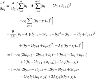
In order to compare different areas of the spectra, we need to have a flat baseline. To do this, we locate the baseline by a method developed for NMR data by Xi and Rocke (2008). For a spectrum with n data points (m_i,y_i), where m_i is the mass and y_i is the height of the i-th data point in the spectrum, define the following score function F:

(1)

where z₊ ≡ max {z,0}, b_i represents the value of the baseline at the i-th data point, and A₁ and A₂ are constants to be determined. We maximize this score function over all possible values of {b_i} to find the baseline.¹

The first term in F represents the overall height of the baseline. The last term is negative only when the baseline is above the data points, so it counteracts the first term and helps ensure that the baseline goes through the middle of the data. The second term is a measure of the curvature of the baseline, so maximizing F will prevent the baseline from curving upward too sharply in areas with peaks.

Xi Rocke show that (assuming normally distributed noise) , where σ is the standard deviation of the noise. They also show that A₁ should have the form A₁ = n⁴A^*₁ / σ for some constant A^*₁. For the data in this article, we experimentally determined the best value of A^*₁ to be approximately 1.1 × 10⁻⁹.

We maximize the score function in Equation (1) by finding the gradient and setting it equal to zero. Let be the indicator function for the set A. Then, for 3 ≤ j ≤ n − 2, we have

(2)

Setting this equal to zero and solving gives us

(3)

For the boundary point j = 2, the term in Equation (2) involving b_j−2 does not appear, so we end up with 5b_j instead of 6b_j and -2b_j−1 instead of -4b_j−1 (and obviously no b_j−2 term) in Equation (3); and similarly for j = n − 1. For j = 1, the terms in Equation (2) involving b_j−1 do not appear, so we end up with b_j − 2b_{j + 1} + b_{j +2} replacing the quantity in brackets in Equation (3); and similarly for j = n. Combining these gives the following linear system for B_{k −1}:

(4)

Here, M is a penta-diagonal matrix with values (1,5,6,6, …,6,6,5,1) on the main diagonal, values (-2,-4,-4, …,-4,-4,-2) on the sub- and super-diagonals and ones on the sub-sub- and super-super-diagonals; J_k is an n × n diagonal matrix with entries

and Y_k is an n × 1 column vector with entries

where b_i,k is the i-th component of B_k. We solve Equation (4) iteratively, starting the iteration with all the entries of B₀ equal to the median of {y_i}. We stop when fewer than 0.1% of the values of change from one iteration to the next or after 30 iterations.

That this calculation is effective in identifying the baseline can be seen by examining the autocorrelation series for a spectrum both pre- and post baseline correction (Fig. 1). Before baseline correction, the autocorrelation does not go to zero, reflecting the fact that the baseline is basically an increasing function of mass. After baseline correction, the autocorrelation does decay to zero. [Extending the autocorrelation plot a little further shows a large (r ≈ 0.25) spike indicating a lag corresponding to isotopes, which obviously have highly correlated values.]

Fig. 1.

The autocorrelation series (starting with lag 7) of a typical spectrum pre-baseline correction (left) and post-baseline correction (right). See Section 2.1.

2.2 Data transformation

With data spanning several orders of magnitude, it is often necessary to apply a logarithmic transformation to the data before using standard statistical tests. In this case, the baseline-adjusted data are sometimes negative, so we instead use a shifted-log transformation:

where log is the natural (base e) logarithm, and c_j = 10 − min_i {y_i^′}, with {y_i^′} the baseline-adjusted data for spectrum j. See Figure 2.

Fig. 2.

Graphs of raw data and baseline-corrected, shifted-log-transformed data (the ‘final data’) for a typical spectrum.

The initial reaction of many people when they see Figure 2 is that the final data look worse than the raw data. It is important to remember, however, that all of the ‘noise’ that appears in the final data is also present in the raw data—it just is obscured by the vertical scale of the graph. By taking the logarithm, we ensure that one peak which is orders of magnitude larger than any other will not dominate the analysis. More importantly, in order to more closely satisfy the assumption of constant error variance that underlies statistical models such as ANOVA and ANCOVA, it is necessary to take logarithms of the data. Even though the final data may look worse than the raw data from a ‘messiness’ perspective, they are actually much better for the purpose of statistical analysis.

2.3 Peak location

We will refer to the baseline corrected, shifted-log-transformed data as the ‘final data’. Once we have the final data, we must locate the compounds they contain. To do this, we observe that the peaks in the final data are nearly parabolic (Fig. 3). Thus, we determine peaks by finding five consecutive points in the final data which, when fitted with a quadratic function by the least-squares method, have correlation satisfying r² ≥ 0.98 and a negative coefficient for x². Writing this in the form

(5)

gives us an estimated mass for the peak of m_i, a height for the peak of h_i and a measure of the width for the peak of w_i.

Fig. 3.

A typical peak in the final data is approximately parabolic. See Section 2.3.

The fact that the peaks are parabolic on the log scale means that they are Gaussian on the raw scale. This is probably due to the Fourier transformation process, which is a type of averaging. The Central Limit Theorem then implies that the resulting averages will be approximately normally distributed, leading to the type of peaks seen in the data. In particular, this method of peak location will probably not be applicable to data generated by other types of mass spectrometry (such as time-of-flight MS).

2.4 Peak selection

Peak selection consisted of a two-step process: locating masses of interest by finding ‘large’ peaks in each spectrum, then calculating the peak heights for all spectra at those interesting masses. It is clear from the data that not every fitted parabola in the final data represents a compound—for example, in one typical prostate cancer spectrum analyzed for this article, we found 104 100 nonoverlapping parabolas that satisfy the criteria in Section 2.3, most of which were clearly in the ‘noise’ part of the spectrum. Thus, for each individual spectrum, we calculated the center c and scale s of the points in the spectrum using Tukey's biweight with K = 6 and only considered so-called ‘large’ peaks—peaks which had h_i ≥ c + 6s, where h_i is the value calculated for the peak in Equation (5). (In other words, large peaks are the peaks which get zero weight when calculating the center and scale.)

Data coming out of the mass spectrometer are not calibrated; peaks representing the same compound can be as far apart as 0.05 Da (or more, depending on the technology used). The mass spectroscopists performed a preliminary calibration to align peaks. At this stage in the analysis, the statisticians performed a second calibration to fine-tune the alignment by taking ‘strong’ peaks—peaks which are large in all spectra—and making their masses agree exactly. We calibrated the remaining masses by using a cubic interpolation spline (interpSpline from the splines package in the R software package) based on the strong peaks.

Once we had this set of peak heights and recalibrated masses, we identified large peaks in different spectra whose masses differed by at most 10 p.p.m. Note that this can lead to identifying two peaks from the same spectrum; for example, if spectrum A has peaks at 1000.01 Da and 1000.025 Da and spectrum B has a peak at 1000.016 Da, then the peak in spectrum B would be identified with both peaks in spectrum A, thus requiring both of the peaks in spectrum A to be the same peak. To avoid this, we identified the peak in spectrum with the closer of the two peaks in spectrum A—in this case, the one at 1000.01 Da.

Not every spectrum had a large peak for every compound, so we had to deal with these initially nondetected peaks. We calculated peak heights for these peaks by taking from the final data (i) the height of a fitted parabola in the same mass range as the nonmissing data (if one was available); or (ii) the largest height in the correct mass range (if no peak was available); or (iii) the height at the closest mass to the nonmissing values. The result was a list of heights for each presumed compound that had a large peak in at least one of the spectra. This list of heights was what we used for statistical testing.

For the breast and prostate cancers data, it was also necessary to combine the replicates for each sample into a single number for each subject. Because of the inherent variability in the sample preparation process in MALDI MS, any individual replicate may be missing a peak of the analyte—as an extreme case, if there were a large clump of the matrix at the spot the laser hit, then the entire spectrum would be based on the matrix, not the analyte. Careful sample preparation can reduce this variability but not eliminate it entirely. It is therefore reasonable to assume that any peak which appears in one of the replicates is actually in the sample, and that a reasonable way to combine replicates is to use the maximum value (as opposed to the median or mean as would typically be used) of each peak over the set of replicates. To confirm the choice of the maximum, we tried combining the replicates in three additional ways: second largest value, median and mean. These methods gave results comparable to those obtained from using the maximum, but (as expected) the analyses derived from them were not as sensitive.

2.5 Normalization

We tried three methods to normalize the spectra. The first was not to normalize at all. In the second, we normalized each spectrum using the average height of all large peaks from that spectrum. In the third, we normalized each spectrum using the average height of the strong peaks in that spectrum. (Simply normalizing by using the average height in each spectrum was not tried because the average heights of the final data were nearly the same in all spectra. Thus, such a normalization scheme would not have been noticeably different from not normalizing at all.) For the prostate cancer samples and the second method, we tried normalizing both before and after combining replicates.

We normalized additively on the final data (which is roughly equivalent to normalizing multiplicatively on the raw data). For example, in the third method, if H_ij is the height of the j-th strong peak in spectrum i for the final data, then each height h in spectrum i would be normalized to be

(6)

If there are n spectra and m strong peaks, then the values of . and . in Equation (6) are given by Equations (7) and (8).

(7)

(8)

All normalization schemes we tried gave similar results in terms of the final set of significant peaks. The results reported in this article come from using the third normalization method described above before combining replicates.

2.6 Statistical analysis

Since the cancer and control groups were not age matched, we used an ANCOVA model with age as a covariate to test the effect of cancer status, once age effects have already been taken into account. We obtained a P-value for each compound from the F-test of the significance of cancer status given that age was already in the model. Since we were dealing with thousands of compounds under each scenario, we corrected for multiple testing using the method of Benjamini and Hochberg (1995) to control the false discovery rate (FDR) at 0.1.

The Benjamini–Hochberg method can be highly sensitive to the set of starting P-values. Since (ideally) biomarkers should be strongly present in at least one of the groups analyzed, we confined our attention to those compounds which had a large peak in at least K spectra, where K was a number to be determined. For each dataset, we calculated the set of significant differences for all possible values of K (from one to the total number of spectra). For the prostate cancer data, due to the relatively small sample size (20 subjects), we used all significant peaks found with any value of K. For the breast and ovarian cancers data, we started with all compounds that had large peaks in at least 75% of the spectra—i.e. 165 for each fraction of the breast cancer data and 149, 146 and 148, respectively, for the 10%, 20% and 40% fractions of the ovarian cancer data.

As a check on the P-values obtained by these methods, we ran a permutation test in each experiment on the peaks that were found to be significantly different to get a distribution-free estimate of the P-values. For the breast and ovarian cancers data, we used 100 000 randomly permuted values for the cancer status and found the fraction that gave a more extreme test statistic than the actual covariates. For the prostate cancer data, we tried all ways of dividing the subjects into two groups.

3 RESULTS

We found only two significant results in the prostate cancer 10% fraction data. Table 2 gives the results for the prostate cancer 20% fraction data, which are illustrative of the results for the remaining six datasets. The masses labeled with asterisks are known glycans; the remaining masses could be unknown glycans, peptides, ion fragments, etc. (For full details of the results as well as the biological implications, see forthcoming papers by the authors.)

Table 2.

Masses for which cancer status is significant after adjusting for age effects in the prostate cancer data, 20% fraction

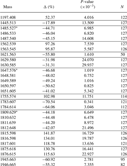Those marked with asterisks represent known glycans. Δ > 0 means upregulated in the cancer group and is roughly the percentage difference on the raw scale. P-values are not adjusted for multiple testing. N is the number of spectra (out of 127) with a large peak at the given mass. Horizontal lines separate presumed isotope groupings. See Section 3.

The permutation tests gave similar P-values to the actual tests used. We first removed five peaks in the prostate cancer, 20% fraction, dataset and one peak in the breast cancer, 20% fraction, dataset that had the permutation test P-values much smaller than the ANCOVA P-values. In each of the seven experiments that had more than two significant results, we then fit a linear model of the form P = Ca to the significant P-values, where P represents the P-value obtained from the permutation test and a represents the P-value from ANCOVA. For the ovarian and breast cancer sets (with their large sample sizes), the resulting estimates for C ranged from 0.984 to 1.007 and the correlations obtained were all at least 0.9994. The prostate cancer permutation tests were less well behaved (probably due to the much smaller sample size), but we still obtained estimates C = 1.066 with correlation 0.9988 in the 20% fraction and C = 0.930 with correlation 0.9744 in the 40% fraction. (Although the value of C in the last case was not as close to 1 as the others, the 95% confidence interval for C did contain 1.) Overall, this is strong evidence that the P-values obtained from the ANCOVA model are valid. See Figure 4 for a typical scatterplot of P-values.

Fig. 4.

The dashed line is the line y =x. Each point represents a peak that was declared statistically significant based on Benjamini–Hochberg with FDR 0.1 using the ANCOVA P-value (see Table 2). The five points in the lower right (four of which represent different isotope peaks of the same compound) were removed before calculating the regression line and correlation described in the text. See Section 3.

In addition, we found two distinct compounds (both with isotope sequences) that were significantly different in the 20% fraction in all three types of cancer. These are listed in Table 3.

Table 3.

Masses for which cancer status is significant after adjusting for age effects for the 20% fraction in all three types of cancer studied

Mass (Da)	Breast	Ovarian		Prostate
	Δ (%)	Δ B (%)	Δ C (%)	Δ (%)
1485.527*	109.67	71.27	106.06	−44.71
1486.533	112.88	73.64	110.48	−46.04
1487.540	121.13	71.31	105.07	−45.15
1809.629 *	−27.95	−22.66	−38.54	−44.18
1810.632	−28.48	−22.57	−38.69	−44.48
1811.639	−30.04	−23.15	−39.20	−44.20
1812.648	−32.73	−23.12	−40.35	−42.07

Those marked with asterisks represent known glycans. Δ >0 means upregulated in cancer and is roughly the percentage difference on the raw scale. Δ B and Δ C are the differences from borderline tumor patients and cancer patients, respectively, to normal subjects. Horizontal lines separate presumed isotope groupings. See Section 3.

4 DISCUSSION

The techniques we have developed appear to be effective in the analysis of MALDI FT-ICR mass spectrometry data. The fact that entire isotope sequences (e.g. lines 11–15 in Table 2) are significant together and have roughly the same estimated Δ and P-value is a strong indicator of the reliability of the techniques. The fact that the permutation tests and ANCOVAs give rise to virtually identical P-values indicates that the statistical modeling assumptions are reasonable.

The single most interesting aspect of the analysis was the discovery of masses that are significantly different in the 20% fraction between cancer and control patients in all three types of cancer (see Table 3). The significantly different masses form two isotope series representing known glycans (Hex₃HexNAc₄Fuc₁ and Hex₅HexNAc₄Fuc₁) which are structurally related by the addition of two hexose groups. Table 4 takes the primary peaks of those two glycans plus the intermediate related glycan Hex₄HexNAc₄Fuc₁ and displays the estimated differences in each of the three types of cancer. There appears to be a difference in the responses of men and women to cancer; note that the relative levels of the three glycans in prostate cancer are approximately the same, while in breast and ovarian cancers they transition from highly overexpressed to highly underexpressed in cancer as the glycans become more massive. It would be interesting to analyze a mixed-gender cancer set (e.g. colon or lung cancer) to explore whether these observations are merely coincidence or indicative of some general systemic response to cancer.

Table 4.

Three related glycans and their relative levels in the 20% fractions of each of the three types of cancer studied

Glycan	Breast	Ovarian		Prostate
	Δ (%)	Δ B (%)	Δ C (%)	Δ (%)
Hex3NAc4Fuc1	109.67	71.27	106.06	−44.71
Hex4NAc4Fuc1	10.88	11.13	6.89	−46.68
Hex5NAc4Fuc1	-27.95	-22.66	-38.54	-44.18

Δ > 0 means upregulated in cancer and is roughly the percentage difference on the raw scale. Δ B and Δ C are the differences from borderline tumor patients and cancer patients, respectively, to normal subjects. See Section 4.

One possibility for improving the analysis is to deal with isotopes. Currently, we treat isotopes as separate compounds, but by combining them into single peaks, we would undoubtedly gain statistical power. A good example of this is illustrated in Table 5, which comes from a previous analysis (of the prostate cancer, 20% fraction data) which ignored age as a covariate. Note that the isotope sequence of the peak at 1645.576 Da overlaps the isotope sequence of the peak at 1647.576 Da, and that the compound with lower mass is downregulated in cancer while the compound with higher mass is upregulated. The result is that the differences tend to cancel each other out, so the estimated Δ is smaller in absolute value and the P-value is larger for the first few isotopes in the 1647.576 Da sequence than for the later isotopes. (The remnants of this effect can be seen in Table 2: even though the mass at 1645.580 is no longer significant with age as a covariate, we still get the same pattern of effect size and P-value for the mass sequence starting at 1647.576.) In other datasets analyzed for this article, we even see cases due to this phenomenon where the main peak is not significantly different between the groups, but the later isotope peaks are significantly different.

Table 5.

Example of isotope interference from a previous analysis of the prostate cancer, 20% fraction data, without using age as a covariate

Mass	Δ (%)	P-value (× 10−3)	N
1645.580	58.07	18.119	127
1646.586	56.51	16.372	127
1647.576 *	−37.65	3.571	127
1648.581	−38.94	2.807	127
1649.589	−40.48	3.040	127
1650.597	−41.89	2.094	127
1651.605	−35.72	3.905	127

Those marked with an asterisk represents known glycans. Isotope-detection software initially categorized this as one long isotope sequence, although it clearly consists of two overlapping isotope sequences. See Section 4.

Another way to gain statistical power would be to concentrate the analysis on glycans. Kronewitter et al. (submitted for publication) have constructed a theoretical N-linked glycan library and applied it to human serum samples to develop an experimental serum glycan profile. By starting with that profile, we should be able to use a smaller set of P-values in the Benjamini–Hochberg method, which would probably lead to a more sensitive analysis that is limited to the compounds of interest—namely, glycans.

Even without these potential improvements, however, the techniques we have developed appear to be effective in the analysis of MALDI FT-ICR mass spectrometry data.

REFERENCES

- An HJ, et al. Profiling of glycans in serum for the discovery of potential biomarkers for ovarian cancer. J. Proteome Res. 2006;5:1626–1635. doi: 10.1021/pr060010k. [DOI] [PubMed] [Google Scholar]
- Benjamini Y, Hochberg Y. Controlling the false discovery rate: a practical and powerful approach to multiple testing. J. Roy. Stat. Soc. Ser. B. 1995;57:289–300. [Google Scholar]
- Brockhausen I. Pathways of O-glycan biosynthesis in cancer cells. Bba-Gen Subj. 1999;1473:67–95. doi: 10.1016/s0304-4165(99)00170-1. [DOI] [PubMed] [Google Scholar]
- Dall'Olio F, et al. Biosynthesis of the cancer-related sialyl-α2,6-lactosaminyl epitope in colon cancer cell lines expressing β-galactoside α2,6-sialyltransferase under a constitutive promoter. Eur. J. Biochem. 2001;268:5876–5884. doi: 10.1046/j.0014-2956.2001.02536.x. [DOI] [PubMed] [Google Scholar]
- Dennis JW, et al. Protein glycosylation in development and disease. BioEssays. 1999;21:412–421. doi: 10.1002/(SICI)1521-1878(199905)21:5<412::AID-BIES8>3.0.CO;2-5. [DOI] [PubMed] [Google Scholar]
- Gorelik E, et al. On the role of cell surface carbohydrates and their binding proteins (lectins) in tumor metastasis. Cancer Metastasis Rev. 2001;20:245–277. doi: 10.1023/a:1015535427597. [DOI] [PubMed] [Google Scholar]
- Herbert CG, Johnstone RA. Mass Spectrometry Basics. Boca Raton, FL: CRC Press; 2003. [Google Scholar]
- Hollingsworth MA, Swanson BJ. Mucins in cancer: protection and control of the cell surface. Nat. Rev. Cancer. 2004;4:45–60. doi: 10.1038/nrc1251. [DOI] [PubMed] [Google Scholar]
- Leiserowitz GS, et al. Glycomics analysis of serum: a potential new biomarker for ovarian cancer? Int. J. Gynecol. Cancer. 2008;18:470–475. doi: 10.1111/j.1525-1438.2007.01028.x. [DOI] [PMC free article] [PubMed] [Google Scholar]
- Malykh YN, et al. N-glycolylneuraminic acid in human tumours. Biochimie. 2001;83:623–634. doi: 10.1016/s0300-9084(01)01303-7. [DOI] [PubMed] [Google Scholar]
- Park Y, Lebrilla CB. Application of Fourier transform ion cyclotron resonance mass spectrometry to oligosaccharides. Mass Spectrom Rev. 2005;24:232–264. doi: 10.1002/mas.20010. [DOI] [PubMed] [Google Scholar]
- Varki A. N-glycolylneuraminic acid deficiency in humans. Biochimie. 2001;83:615–622. doi: 10.1016/s0300-9084(01)01309-8. [DOI] [PubMed] [Google Scholar]
- Villanueva J, et al. Correcting common errors in identifying cancer-specific serum peptide signatures. J. Proteome Res. 2005;4:1060–1072. doi: 10.1021/pr050034b. [DOI] [PMC free article] [PubMed] [Google Scholar]
- Xi Y, Rocke DM. Baseline correction for NMR spectroscopic metabolomics data analysis. BMC Bioinformatics. 2008;9:324. doi: 10.1186/1471-2105-9-324. [DOI] [PMC free article] [PubMed] [Google Scholar]
- Yamori T, et al. Differential production of high molecular weight sulfated glycoproteins in normal colonic mucosa, primary colon carcinoma, and metastases. Cancer Res. 1987;47:2741–2747. [PubMed] [Google Scholar]
- Zhang L-K, et al. Gross. Accurate mass measurements by Fourier transform mass spectrometry. Mass Spectrom. Rev. 2005;24:286–309. [Google Scholar]