Prediction of kinase-specific phosphorylation sites using conditional random fields

Abstract

Motivation: Phosphorylation is a crucial post-translational protein modification mechanism with important regulatory functions in biological systems. It is catalyzed by a group of enzymes called kinases, each of which recognizes certain target sites in its substrate proteins. Several authors have built computational models trained from sets of experimentally validated phosphorylation sites to predict these target sites for each given kinase. All of these models suffer from certain limitations, such as the fact that they do not take into account the dependencies between amino acid motifs within protein sequences in a global fashion.

Results: We propose a novel approach to predict phosphorylation sites from the protein sequence. The method uses a positive dataset to train a conditional random field (CRF) model. The negative training dataset is used to specify the decision threshold corresponding to a desired false positive rate. Application of the method on experimentally verified benchmark phosphorylation data (Phospho.ELM) shows that it performs well compared to existing methods for most kinases. This is to our knowledge that the first report of the use of CRFs to predict post-translational modification sites in protein sequences.

Availability: The source code of the implementation, called CRPhos, is available from http://www.ptools.ua.ac.be/CRPhos/

Contact: kris.laukens@ua.ac.be

Suplementary Information: Supplementary data are available at http://www.ptools.ua.ac.be/CRPhos/

1 INTRODUCTION

Protein phosphorylation is an essential type of post-translational modification that consists of the addition of a phosphate (PO₄) group to serine (S), threonine (T), tyrosine (Y) and to a lesser extent histidine (H) residues. The process is catalyzed by a group of enzymes called kinases, and can be reverted by phosphatases. Phosphorylation has important implications on the function of a protein. If an enzyme gets phosphorylated its activity may be stimulated or inhibited, for example, leading to altered metabolic fluxes in the case of a metabolic enzyme, or resulting in the modulation of a regulatory effect if the substrate protein plays a regulatory role. The human genome encodes more than 500 different kinases, many of which have been related to cancer and other diseases (Manning et al., 2002). They regulate a diverse range of biochemical pathways and biological functions and are often indispensable signal integrators in a living system. Being one of the most important reversible mechanisms of post-translational modification, phosphorylation is a prevalent subject of research in biochemistry.

A first step towards elucidating the phosphorylation network consists of the determination of the phosphorylated residues in a substrate protein for a given kinase. Revealing the exact position of a phosphorylation in a sequence is essential to get irrefutable evidence for the assignment of a protein as a kinase substrate. It also provides powerful clues for biomedical drug design or other biotechnological applications. Phosphorylation sites on substrates are usually experimentally determined by mass spectrometry-based techniques (reviewed by Jensen, 2004). This has led to several databases of phosphorylation sites, often tied to specific species, such as ‘The Phosphorylation Site Database’ (Gnad et al., 2007), ‘Phospho.ELM’ (Diella et al., 2004, 2008), ‘PhosphoSite’ (Hornbeck, 2004) and ‘PhosPhAt’ (Heazlewood et al., 2008). Performing such experiments, however, remains time consuming, labor intensive and expensive. These disadvantages have been anticipated by the bioinformatics community with the development of predictive models that are trained with experimentally annotated and known phosphorylation sites. These models can be used to predict potential target sequences and thus significantly reduce the number of sequences that need to be verified by mass spectrometry.

Several computational models have been built and applied with varying success to predict phosphorylation sites, including hidden Markov models (HMMs) (Huang et al., 2005b), neural networks (Blom et al., 1999, 2004; Ingrell et al., 2007), group-based scoring method (Xue et al., 2005; Zhou et al., 2004), Bayesian decision theory (Xue et al., 2006), support vector machines (SVMs) (Kim et al., 2004; Plewczynski et al., 2005, 2008; Wong et al., 2007) and algorithms to identify short protein sequence motifs on recognized substrates (Neuberger et al., 2007; Obenauer et al., 2003). Particularly the flanking sequence (typically -4,+4) around the potential sites (S/Y/T) is often used to develop these models. Apart from the protein sequence, some additional information has also been integrated, including disorder information (Iakoucheva et al., 2004), structure information (Blom et al., 1999) and the distribution of the phosphorylated sites (Moses et al., 2007). The majority of the computational models dedicated to predicting phosphorylation sites use the experimentally validated database Phospho.ELM (Diella et al., 2004, 2008) for training and for the evaluation of their performance. Due to the fact that for some particular kinases in Phospho.ELM only a small number of phosphorylated sites is known, the annotated Swiss-Prot database (Boeckmann et al., 2003) is often used in complement to increase the size of the training and testing dataset.

In this article, we introduce a novel machine learning scheme that overcomes several disadvantages associated with existing methods. The model is based on conditional random fields (CRFs) (Lafferty et al., 2001) and allows prediction of phosphorylated sites for each specific kinase separately. The positive and negative datasets are flanking sequences of amino acids around the potentially phosphorylated residues. Information about the chemical classes that individual amino acids belong to is also incorporated. The CRF model is trained from only the positive training dataset. The key idea of this approach is to generate the probability distribution for the positive data samples. This derived distribution takes the probability values of the positive training dataset, calculated from the corresponding learned CRF model, as its values. Within a set of protein sequences, the number of truly phosphorylated sites is always small compared to the number of non-phosphorylated sites. To overcome this difficulty, we apply Chebyshev's Inequality from statistics theory to find high confidence boundaries of the derived distribution. These boundaries are used to select a part of the negative training data, which is then used to calculate a decision threshold based on a user-provided allowed false positive rate. To evaluate the performance of the method, k-fold cross-validations were performed on the experimentally verified phosphorylation dataset. This new method performs well according to commonly used measures.

2 METHODS

CRFs were introduced initially for solving the problem of labeling sequence data that arises in scientific fields such as bioinformatics and natural language processing. In sequence labeling problems, each data item x_i is a sequence of observations {x_i1,x_i2,…,x_iT}. The purpose of the technique is to make a prediction of the sequence labels, that is, y_i={y_i1,y_i2,…,y_iT}, corresponding to this sequence of observations.

So far, in addition to CRFs, some probabilistic models have been introduced to tackle this problem, such as HMMs (Freitag and McCallum et al., 2000) and maximum entropy Markov models (MEMMs) (McCallum, et al., 2000). In this section, we review and compare these models, before motivating and discussing our choice for the CRFs scheme.

2.1 Review of existing models

An HMM is one of the most common methods for performing sequence labeling. It is a generative model that maximizes the joint probability distribution p(X, Y), where X and Y are random variables whose values take on all observation sequences and corresponding label sequences, respectively. To calculate the joint probability, HMMs need to enumerate all possible observation sequences. This is intractable when the number of atomic observations becomes large. Moreover the interacting range between positions in a sequence is often long. First-order HMMs relax these strict constraints by working with two assumptions. The first one is the fact that a prediction of a future observation only depends on the present one (or on the immediate previous one). As a result we have p(X_t+1∣X_t,X_t−1,…,X₁)=p(X_t+1∣X_t). The second assumption is the time invariant or stationary: p(X_t+1∣X_t)=p(X₂∣X₁).

These limitations of HMMs in particular and generative models in general are the motivation behind the introduction of conditional models. By maximizing the conditional probability p(Y∣X) from the training dataset, conditional models do not explicitly model the observation sequences. Furthermore, these models remain valid if dependencies between arbitrary features exist in the observation sequences, and they do not need to account for these arbitrary dependencies. The probability of a transition between labels may not only depend on the current observation but also on past and future observations. MEMMs (McCallum et al., 2000) are a typical group of conditional probabilistic models. Each state in a MEMM has an exponential model that takes the observation features as input, and outputs the distribution over the possible next states. These exponential models are trained by an appropriate iterative scaling method in the maximum entropy framework.

On the other hand, MEMMs and non-generative finite state models based on next-state classifiers are all victims of a weakness called label bias (Lafferty et al., 2001). In these models, the transitions leaving a given state compete only against each other, rather than against all other transitions in the model. The total score mass arriving at a state must be distributed and observed over all next states. An observation may affect which state will be the next, but does not affect the total weight passed on to it. This will result in a bias in the distribution of the total score weight at a state with fewer next states. In particular, if a state has only one out-going transition, the total score weight will be transferred regardless of the observation. A simple example of the label bias problem has been introduced in the work of Lafferty et al. (2001).

2.2 Conditional random fields

CRFs are discriminative probabilistic models that not only inherit all advantages of MEMMs but also overcome the label bias weakness. While MEMMs use exponential models of the current state to calculate the conditional probabilities of the next states, CRFs use a single exponential model for the conditional probability of all training labels, given the observation sequence. Therefore, the weight of an arbitrary feature can be learned from its global interactions with all the other features. This means that the weights of all the features within CRFs can be traded-off against each other. CRFs have been applied to some common problems in natural language processing, such as NP (noun phrase)-chunking, POS (part of speech)-tagging and text segmentation (Sha and Pereira, 2003), and the experimental results are significantly better than those from HMMs and MEMMs.

In CRFs, the dependencies between the label components of a random variable Y are represented by an undirected graph G=(E,V). Let C be a set of cliques in graph G. Suppose that there exists a set of K feature functions f_k (c,X) predefined in each clique c∈C, where . According to the Hammersley–Clifford theorem, the conditional probability of a label sequence given the observation sequence is calculated as follows (Sha and Pereira, 2003):

(1)

Here Z_o is the normalization function defined over all possible label sequences and φ(c,X) is called the potential function of clique c. This is a non-negative real-valued function and is defined as follows:

(2)

The parameters α_k are learned globally from a labeled training dataset. Although the graph G of Y may have a general structure for the problem of modeling the sequence the most simple and important structure is the linear chain structure. Several authors have previously applied CRFs with a linear structure and obtained good performances (Lafferty et al., 2001; Sha and Pereira, 2003). Within a linear structure, each clique is an edge with two end points. The conditional probability formula can then be rewritten as follows:

(3)

In this formula Y∣_e, Y∣_v are components of the random variable Y corresponding to the edges and vertices of graph G, respectively. The function g_k and h_k are the respective feature functions for the state–observation pair and the state–state pair. These are real-valued functions but are often defined as Boolean functions. In the domain of phosphorylation site prediction, these feature functions, g₁ for example, can be defined as follows:

(4)

Here AA₋₃=“R” means ‘The amino acid three positions left from current AA is R’ and L(AA₀)=“Phos” means ‘The label of the current amino acid is phosphorylated’.

As explained in the Section 3.1, the state–state pair feature functions (h_k in formula 3) are not declared in our implementation. Several authors have proposed methods to efficiently induce such feature functions from datasets (Lafferty et al., 2001; McCallum, 2003; Pietra et al., 1997).

The weights of the CRFs are learned from the training dataset {x_i,y_i} to maximize the conditional log likelihood of label sequences {y_i} (Sha and Pereira, 2003).

(5)

This likelihood function in CRFs is convex when the training label sequences (i.e. a series of the labels ‘phosphorylated’ and ‘non-phosphorylated’) make the state sequences (i.e. a series of amino acids) unambiguous (McCallum, 2003). In the case of phosphorylation site prediction this means that the training labels do corroborate the substrate specificity of the kinase. This situation happens often in practice. It guarantees that the global maximum value of the log likelihood of the conditional probability L will be found.

2.3 Proposed algorithm

In this section, we introduce an algorithm that has all of the advantages of the CRFs discussed in the above section. The algorithm follows a novelty detection approach, as previously successfully implemented in gene prioritization by De Bie et al. (2007). It builds a CRF model M⁺ for all training data objects that belong to the positive class. In this application, we designed the features or patterns according to the motifs described in the biochemical literature on phosphorylation site prediction (reviewed by Kobe et al., 2005). All patterns used are listed in the Supplementary Material. If this set of features and patterns is well designed, the probabilities p(+∣x, M⁺) that a positive training data object x is labeled as positive (+) are guaranteed to be the global maximum. This is due to the convex characteristic of the conditional log likelihood function in CRFs. They will distribute mainly near the largest probability value 1. Furthermore, according to Chebyshev's Inequality (Ewens and Grant, 2001), given a random variable X and a real number n>0, p(∣X−E(X)∣≥nσ)≤1/n². Here E(X)and σ² denote the expected value and the variance of variable X, respectively. This means that the confidence degree of a value of X belonging to the range [E(X)−n*σ,E(X)+n*σ] is larger than (1−1/n²). For example, with n=3, the confidence degree is >89%. From now this interval will be referred to as the n-confidence interval. When applied to the distribution of the probability values p(+∣x, M⁺), the expected value can be estimated by the average value of all values p(+∣x, M⁺), with x being the positive training data objects. The n-confidence interval is enlarged by increasing the value n until the upper bound equals 1. This interval is used in the proposed algorithm to overcome the difficulty that the number of examples in the positive training dataset is very small. Due to the guarantee of obtaining the global maximum of the CRFs, the n-confidence interval is expected to contain all values p(+∣x, M⁺) of all real positive data objects.

Moreover, the negative training dataset may contain some phosphorylated residues that have not yet been experimentally verified as such. These negative data will then get high probabilities—within the n-confidence interval—of being labeled as positive, and will not be considered during the process of controlling the false positive rate of the obtained classifier.

A new data object will be classified as positive if the probability of classifying it as positive given the model M⁺ is greater than or equal to the threshold θ.

In all experiments, we used the open source software tool CRF++http://crfpp.sourceforge.net/ to build the model.

3 RESULTS AND DISCUSSION

3.1 Implementation

We used the Phospho.ELM (Diella et al., 2008) (version 0707) database to experimentally evaluate our approach. This dataset has been used as a benchmark to test the performance of most computational phosphorylation prediction models previously published. Phospho.ELM contains experimentally verified phosphorylation sites in eukaryotic proteins, manually curated from the literature. It stores information about substrate proteins with the exact positions of the residues that are experimentally verified to be phosphorylated by a given kinase. For each potentially phosphorylated residue (S, T or Y), we extracted the nine amino acid sequence, including the central residue, surrounding it (from -4 to +4). All of these sequences of which the central residue was annotated as phosphorylated by a given kinase were considered as the positive set, whereas all remaining 9mer sequences on the same substrate proteins, were considered as negative examples. Following Kim et al. (2004), we discarded highly homologous sequences (over 70% identity) from the positive and negative training dataset to avoid overestimation on accuracy when cross-validating. Such bias appears if the testing data are highly homologous to the training data. The number of positive and negative samples for different kinases, after removing the redundancies, is shown in Table 1. There are clearly much more negative samples than positive ones. Apart from the amino acid itself, the chemical/structural group that an amino acid belongs to is used as an additional feature for each residue. Twenty amino acids were grouped into eight different clusters (Table 2) according to their common chemical/structural properties (Wong et al., 2007). For each position in the positive sequence data, a set of Boolean value feature functions was declared, including functions for amino acids (e.g. formula 4), for chemical groups (e.g. formula 6) and for combinations of amino acids and chemical groups (e.g. formula 7).

(6)

(7)

Here G₋₃=“Sulfur”means ‘The chemical group of the amino acid (AA) three positions left from the current AA belongs to the cluster Sulfur’ and L(AA₀)=“Phos” means ‘The label of the current amino acid is phosphorylated’.

Table 1.

The size of positive and negative datasets for some common protein kinases, obtained from Phospho.ELM version 0707

Protein kinase	Positive size	Negative size
Abl(Proto-oncogene tyrosine-protein kinase)	45	1209
ATM (Ataxia telangiectasia mutated)	55	1882
CaM-KII (Calcium/calmodulin-dependent protein kinases)	50	1829
CDK (Cyclin-dependent kinases)	104	1990
CK1 (Casein kinases 1)	42	1051
CK2 (Casein kinases 2)	226	3875
DNA-PK (DNA-dependent protein kinase catalytic subunit)	20	632
EGFR (Epidermal growth factor receptor)	44	823
Fyn (Proto-oncogene tyrosine-protein kinase)	48	1409
GSK-3 (Glycogen synthase kinases 3)	32	866
InsR (Insulin receptor)	44	724
Met (Hepatocyte growth factor receptor)	13	132
mTOR (FK506 binding protein 12-rapamycin associated protein 1)	13	50
PKA (cAMP-dependent protein kinase)	310	8823
PKB (Protein kinases B)	79	3563
PKC (Protein kinase)	227	4428
Src (Proto-oncogene tyrosine-protein kinase)	141	2681
Syk (Tyrosine-protein kinase)	45	680

Table 2.

The chemical classes to which the 20 amino acids belong, based on Wong et al. (2007)

Group name	Amino Acids
Sulfur	C, M
Aliphatic 1	A, G, P
Aliphatic 2	I, L, V
Acid	D, E
Base	H, K, R
Aromatic	F, W, Y
Amide	N, Q
Small hydroxy	S, T

When applying the algorithm (Section 2.3) to build a predictive model from the positive (i.e. central residue is phosphorylated) and negative (i.e. central residue is not phosphorylated) sequence data, the conditional probabilities in Steps 4 and 7 are probabilities of the central residues in the sequence data having the label ‘Phos’ (i.e. ‘phosphorylated’). These probabilities are equivalent to the total sum of the probabilities of all possible label sequences of which the central labels are ‘Phos’, assigned by a CRF given the flanking sequence of amino acids. This increases the computational complexity of the algorithm due to the required enumeration of all possible surrounding labels.

To tackle this problem, we introduce a transferring method that is applied to the sequence data as follows. Each nine-residue long amino acid sequence is represented in an equivalent form, where the center residue (S, Y or T) is a data object and the surrounding residues themselves and their corresponding features become the new features (Fig. 1). The information about the positions of the residues is conserved, thus the CRF model still has the ability to exploit the meaning of residue positions if suitable feature functions (g_k) are used. The state–state feature functions (h_k, formula 3) are not further declared since the dependencies between labeling information of the surrounding amino acids is omitted in this new representation.

Fig. 1.

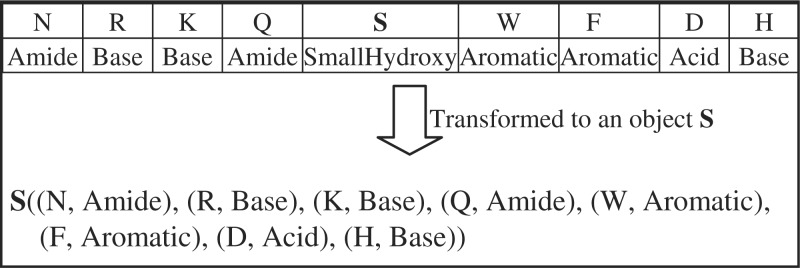
Method for transforming an amino acid sequence to a data object of the central amino acid.

3.2 Evaluation

To evaluate the performance of the algorithm, k-fold cross-validation was used for the model trained from the large datasets, whereas Jackknife cross-validation was applied when the models were trained with less than 30 positives. Each cross-validation was performed 20 times, and after each round we calculated Sensitivity (Sn)=TP/(TP+FN) and Specificity (Sp)=TN/(TN+FP). Here TP, TN, FP and FN are true positive, true negative, false positive and false negative values, respectively. The average values after 20 runs were used as the final measure of the performance for the model.

For each kinase-specific phosphorylation predictor, the ROC (receiver operating characteristic) curve, which shows the tradeoff between sensitivity and specificity, was generated from the final average. The ROC curves obtained from different k-fold cross-validations (k=2, 4, 6, 8, 10) were approximately the same (data not shown). For the sake of clarity, all shown ROC curves are the result from 10-fold cross-validation (Fig. 3 and Supplementary figures, blue lines). All ROC curves, except CDK1 and PKB, reach 100% sensitivity with a specificity of at least 20%. Because the number of positives is much smaller than the number of negatives, this implies a significant reduction in the number of required validations, even if no false negatives are desired.

Fig. 3.

ROC curves of our method for some well-studied kinases, using 10-fold cross-validation (CRPhos). CRF* stands for the equivalent curve for a CRF model learned from both the positive and negative training dataset. For comparison, corresponding performance measures reported in literature are shown: PPSP (Xue et al., 2006), Scansite (Obenauer et al., 2003), NetPhosK (Blom et al., 2004), KinasePhos 1.0 (Huang et al., 2005a), KinasePhos 2.0 (Wong et al., 2007), GPS (Zhou et al., 2004) and PredPhospho (Kim et al., 2004).

We also validated whether the observed specificity value of a classifier generated from the method is close to the expected value. For each value of an expected specificity, a 4-fold cross-validation procedure was implemented 20 times. The average observed specificity was calculated and compared with the expected value (Fig. 2). These values were identical for kinases with a negative training dataset larger than 1500. For kinases with a smaller negative training set, the smallest regression coefficient was 0.97, for the ‘mTOR’ kinase, of which the number of negative training sequences was only 50. As a consequence, the algorithm can return any desired point (classifier) on the ROC curve based on taking into account an expected specificity value as input.

Fig. 2.

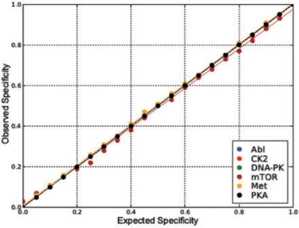
Relation between expected and observed specificity values of obtained predictor. All lines are generated using linear regression.

The model proposed in this article uses the positive dataset for training, and uses the negative data to calculate a decision threshold. In order to demonstrate the efficiency of this approach, we also tested a conventional approach, using both the positive and negative data for training a CRF model. For this experiment, the nine amino acid protein sequences from both the positive and the negative dataset were taken as input to the learning algorithm of the CRFs. The derived ROC curves are shown in red in Figure 3 and in the Supplementary Material. For most kinases, this conventional approach results in a slightly worse ROC curve, indicating that our approach outperforms the application of CRFs trained on both positive and negative data.

3.3 Comparison

The derived ROC curves allow for easy comparison of our method with reported performance measures from other methods. We followed two different approaches.

The approach applied by most authors of phosphorylation site prediction methods, is the direct comparison of obtained results with previously reported performances (Huang et al., 2005a; Kim et al., 2004; Zhou et al., 2004). If available, performance values, reported in literature as pairs of sensitivities/specificities, were shown as colored dots on the ROC plots for each kinase method (Fig. 3 and Supplementary Fig. 1). These values can be considered worse or better, depending on whether these dots fall below or above the CRPhos ROC curve, respectively. In most cases, CRPhos yielded a performance that is comparable or better than other methods. (SVMs-based approaches applied in Predphospho (Kim et al., 2004) and KinasePhos 2.0 (Wong et al., 2007) do perform better in some instances (e.g. both in CK2, KinasePhos 2.0 in PKC, PredPhospho in CDK), but worse in other cases (both in PKA, PredPhospho in PKC). However, both predictors have been validated on data of which the size of the negative and positive subset has been equalized, in contrast to this article. Compared with PPSP (Xue et al., 2006), CRPhos performs better for the majority of the kinases, but worse or similar for a few. From all kinases, only the prediction for CK2 by CRPhos is generally worse than those by other prediction methods, although even then CRPhos achieves both sensitivity and specificity values above 80%. NetphosK could only be compared for PKA and ATM, yielding worse and better performance, respectively. Except for CK2, CRPhos performs similar or better than the other methods, including GPS (Zhou et al., 2004), Scansite (Obenauer et al., 2003) and KinasePhos 1.0 (Huang et al., 2005a).

There is a chance that the version of the dataset, which is different for previously published models, affects the above comparison. An ideal solution to perform an unbiased comparison is running new cross-validations on all existing methods using the same dataset that we used. This is practically hard to achieve since trainable versions of most tools are not available. An alternative solution consists of testing and comparing our method and other existing ones on the same testing dataset. There is however a high chance to get a biased comparison if some testing data are already learned by one of the methods.

To eliminate this problem, a more rigorous approach was recently deployed by Wan et al. (2008). They generated a subset of Phospho.ELM, called MetaPS06, which contains the phosphorylation sites that were only recently added, after publication of existing prediction models. This MetaPS06 set does not overlap with any previously used training data. By testing this dataset against different prediction tools, Wan and Colleagues (2008) obtained comparable performance measurements that represent the predictive power of each tool. To generate equivalent performance values, we removed from Phosphos.ELM version 07 all phosphorylated sites originated from Phospho.ELM version 06 (with annotation data <12/31/2004), as described (Wan et al., 2008). For this experiment the removed dataset was used to train the CRPhos model, whereas the remaining fraction was used for testing. The results (Fig. 4) demonstrate that the performance of CRPhos remains better than the performance of most other methods. Unlike other methods, CRPhos learns the model only from the ‘golden’ positive dataset and not from the ‘un-golden’ negative dataset. This negative dataset could contain some real phosphorylated (positive) data that have not yet been experimentally validated. This may cause a bias in the prediction by models that are trained from both positive and negative data.

Fig. 4.

Performance of CRPhos with the testing dataset that is created according to the scheme in Wan et al. (2008). The remaining dataset after removing this testing data from Phospho.ELM v.07 was used to train CRPhos. The performance measure of other existing methods, reported by Wan et al. (2008), are shown for comparison.

Moreover, we also cross-validated our model using the older versions of Phospho.ELM. versions 06 & 1206. Supplementary Figure 2 demonstrates that this has almost no effect on the performance.

A significant advantage of the method described in this article lies in the fact that it is able to generate predictions for all possible specificity values. Any classifier, defined by a point in the ROC curve, can be readily obtained, whereas other approaches are only able to generate one classifier with a fixed sensitivity/specificity.

4 CONCLUSION

In this article, we introduced a novel approach based on CRFs to predict kinase-specific phosphorylation sites. Upon validation with a real dataset of phosphorylation sites, the method yielded accurate predictions that were similar or better than predictions obtained with existing methods. This is consistent with the theoretical advantages of CRFs, including the convergence to the global maximum of the log likelihood conditional probability and the capability of capturing all amino acid motifs and their interactions in a global fashion.

Our approach employs Chebyshev's Inequality to find the confidence interval for the distribution of the real positive data. As a result, it overcomes the difficulty that, in reality, the size of the experimentally verified positive data is very small compared to that of the negative data. Moreover, the use of Chebyshev's Inequality also allows eliminating the noisy negative data, which may contain target sites that have not yet been experimentally assigned as positive.

Finally, this method allows obtaining an optimal prediction for any given allowed false positive rate. This gives the end-user extra flexibility, especially when applied in situations where either incomplete detection, or false positives are undesired.

REFERENCES

- Blom N, et al. Sequence and structure-based prediction of eukaryotic protein phosphorylation sites. J. Mol. Biol. 1999;294:1351–1362. doi: 10.1006/jmbi.1999.3310. [DOI] [PubMed] [Google Scholar]
- Blom N, et al. Prediction of post-translational glycosylation and phosphorylation of proteins from the amino acid sequence. Proteomics. 2004;4:1633–1649. doi: 10.1002/pmic.200300771. [DOI] [PubMed] [Google Scholar]
- Boeckmann B, et al. The Swiss-Prot protein knowledgebase and its supplement TrEMBL in 2003. Nucleic Acids Res. 2003;31:365–370. doi: 10.1093/nar/gkg095. [DOI] [PMC free article] [PubMed] [Google Scholar]
- De Bie T, et al. Kernel-based data fusion for gene prioritization. Bioinformatics. 2007;23:i125–i132. doi: 10.1093/bioinformatics/btm187. [DOI] [PubMed] [Google Scholar]
- Diella F, et al. Phospho.ELM: a database of experimentally verified phosphorylation sites in eukaryotic proteins. BMC Bioinformatics. 2004;5:79. doi: 10.1186/1471-2105-5-79. [DOI] [PMC free article] [PubMed] [Google Scholar]
- Diella F, et al. Nucleic Acids Res. 2008;36:D240–D244. doi: 10.1093/nar/gkm772. [DOI] [PMC free article] [PubMed] [Google Scholar]
- Ewens WJ, Grant GR. Statistical Methods in Bioinformatics: An Introduction. Philadelphia, PA: Springer; 2001. [Google Scholar]
- Freitag D, McCallum A. Proceedings of the Seventeenth National Conference on Artificial Intelligence and Twelfth Conference on Innovative Applications of Artificial Intelligence. AAAI Press/The MIT Press; 2000. Information extraction with HMM structures learned by stochastic optimization; pp. 584–589. Available at http://portal.acm.org/citation.cfm?id=723414&dl=GUIDE. [Google Scholar]
- Gnad F, et al. PHOSIDA (phosphorylation site database): management, structural and evolutionary investigation, and prediction of phosphosites. Genome Biol. 2007;8:R250. doi: 10.1186/gb-2007-8-11-r250. [DOI] [PMC free article] [PubMed] [Google Scholar]
- Heazlewood JL, et al. PhosPhAt: a database of phosphorylation sites in Arabidopsis thaliana and a plant specific phosphorylation site predictor. Nucleic Acids Res. 2008;36:1015–1021. doi: 10.1093/nar/gkm812. [DOI] [PMC free article] [PubMed] [Google Scholar]
- Hornbeck PV. PhosphoSite: a bioinformatics resource dedicated to physiological protein phosphorylation. Proteomics. 2004;4:1551–1561. doi: 10.1002/pmic.200300772. [DOI] [PubMed] [Google Scholar]
- Huang HD. KinasePhos: a web tool for identifying protein kinase-specific phosphorylation sites. Nucleic Acids Res. 2005a;33:226–229. doi: 10.1093/nar/gki471. [DOI] [PMC free article] [PubMed] [Google Scholar]
- Huang HD, et al. Incorporating hidden Markov model for identifying protein kinase-specific phosphorylation sites. J. Comput. Chem. 2005b;26:1032–1041. doi: 10.1002/jcc.20235. [DOI] [PubMed] [Google Scholar]
- Iakoucheva LM, et al. The importance of intrinsic disorder for protein phosphorylation. Nucleic Acids Res. 2004;32:1037–1049. doi: 10.1093/nar/gkh253. [DOI] [PMC free article] [PubMed] [Google Scholar]
- Ingrell CR, et al. NetPhosYeast: prediction of protein phosphorylation sites in yeast. Bioinformatic. 2007;7:895–897. doi: 10.1093/bioinformatics/btm020. [DOI] [PubMed] [Google Scholar]
- Jensen ON, et al. Modification-specific proteomics: characterization of post-translational modifications by mass spectrometry. Curr. Opin. Chem. Biol. 2004;8:33–41. doi: 10.1016/j.cbpa.2003.12.009. [DOI] [PubMed] [Google Scholar]
- Kim JH, et al. Prediction of phosphorylation sites using SVMs. Bioinformatics. 2004;20:3179–3184. doi: 10.1093/bioinformatics/bth382. [DOI] [PubMed] [Google Scholar]
- Kobe B, et al. Substrate specificity of protein kinases and computational prediction of substrates. Biochim. Biophys. Acta. 2005;1754:200–209. doi: 10.1016/j.bbapap.2005.07.036. [DOI] [PubMed] [Google Scholar]
- Lafferty JD, et al. Proceedings of the Eighteenth International Conference on Machine Learning. San Francisco, CA, USA: Morgan Kaufmann Publishers Inc; 2001. Conditional random fields: probabilistic models for segmenting and labeling sequence data; pp. 282–289. [Google Scholar]
- Manning G, et al. The protein kinase complement of the human genome. Science. 2002;298:1912–1934. doi: 10.1126/science.1075762. [DOI] [PubMed] [Google Scholar]
- McCallum A. Proceedings of the 19th Conference in Uncertainty in Articifical Intelligence. Acapulco, Mexico: Morgan Kaufmann; 2003. Efficiently inducing features of conditional random fields; pp. 403–410. [Google Scholar]
- McCallum A, et al. Proceedings of ICML 2000. California: Stanford; 2000. Maximum entropy Markov models for information extraction and segmentation; pp. 591–598. [Google Scholar]
- Moses AM, et al. Spatial clustering of phosphorylation site recognition motifs can be exploited to predict the targets of cyclin-dependent kinase. 2007;8:R23. doi: 10.1186/gb-2007-8-2-r23. [DOI] [PMC free article] [PubMed] [Google Scholar]
- Neuberger G, et al. pkaPS: prediction of protein kinase A phosphorylation sites with the simplified kinase-substrate binding model. Biol. Direct. 2007;2:1. doi: 10.1186/1745-6150-2-1. [DOI] [PMC free article] [PubMed] [Google Scholar]
- Obenauer JC, et al. Scansite 2.0: proteome-wide prediction of cell signaling interactions using short sequence motifs. Nucleic Acids Res. 2003;31:3635–3641. doi: 10.1093/nar/gkg584. [DOI] [PMC free article] [PubMed] [Google Scholar]
- Pietra DS, et al. Inducing features of random fields. IEEE Trans. Pattern Anal. Match. Intell. 1997;19:380–393. [Google Scholar]
- Plewczynski D, et al. A support vector machine approach to the identification of phosphorylation sites. Cell. Mol. Biol. Lett. 2005;10:73–89. [PubMed] [Google Scholar]
- Plewczynski D, et al. Automotif server for prediction of phosphorylation sites in proteins using vector machine. J. Mol. Model. 2008;14:69–76. doi: 10.1007/s00894-007-0250-3. [DOI] [PubMed] [Google Scholar]
- Sha F, Pereira F. Proceedings of the 2003 Human Language Technology Conference and North American Chapter of the Association for Computational Linguistics. Morristown, NJ, USA: Association for Computational Linguistics; 2003. Shallow parsing with conditional random fields. (HLT/NAACL-03) [Google Scholar]
- Wan J, et al. Meta-prediction of phosphorylation sites with weighted voting and restricted grid search parameter selection. Nucleic Acids Res. 2008;36:e22. doi: 10.1093/nar/gkm848. [DOI] [PMC free article] [PubMed] [Google Scholar]
- Wong YH, et al. KinasePhos 2.0: a web server for identifying protein kinase-specific phosphorylation sites based on sequences and coupling patterns. Nucleic Acids Res. 2007;35:W588–W594. doi: 10.1093/nar/gkm322. [DOI] [PMC free article] [PubMed] [Google Scholar]
- Xue Y, et al. GPS: a comprehensive www server for phosphorylation sites prediction. Nucleic Acids Res. 2005;33:W184–W187. doi: 10.1093/nar/gki393. [DOI] [PMC free article] [PubMed] [Google Scholar]
- Xue Y, et al. PPSP: prediction of PK-specific phosphorylation site with Bayesian decision theory. BMC Bioinformatics. 2006;7:163. doi: 10.1186/1471-2105-7-163. [DOI] [PMC free article] [PubMed] [Google Scholar]
- Zhou FF, et al. GPS: a novel group-based phosphorylation predicting and scoring method. Biochem. Biophys. Res. Commun. 2004;325:443–1448. doi: 10.1016/j.bbrc.2004.11.001. [DOI] [PubMed] [Google Scholar]
Associated Data
This section collects any data citations, data availability statements, or supplementary materials included in this article.