Estimating the capacity for improvement in risk prediction with a marker

Abstract

Consider a set of baseline predictors X to predict a binary outcome D and let Y be a novel marker or predictor. This paper is concerned with evaluating the performance of the augmented risk model P(D = 1|Y,X) compared with the baseline model P(D = 1|X). The diagnostic likelihood ratio, DLR_X(y), quantifies the change in risk obtained with knowledge of Y = y for a subject with baseline risk factors X. The notion is commonly used in clinical medicine to quantify the increment in risk prediction due to Y. It is contrasted here with the notion of covariate-adjusted effect of Y in the augmented risk model. We also propose methods for making inference about DLR_X(y). Case–control study designs are accommodated. The methods provide a mechanism to investigate if the predictive information in Y varies with baseline covariates. In addition, we show that when combined with a baseline risk model and information about the population distribution of Y given X, covariate-specific predictiveness curves can be estimated. These curves are useful to an individual in deciding if ascertainment of Y is likely to be informative or not for him. We illustrate with data from 2 studies: one is a study of the performance of hearing screening tests for infants, and the other concerns the value of serum creatinine in diagnosing renal artery stenosis.

1. INTRODUCTION

One of the goals of current biomedical research is to develop better methods for individual risk prediction. New genomic, proteomic, and imaging technologies in particular promise to provide tools for accurate assessment of risk. These tools could be used in diagnostic settings to determine which patients are at high risk of having disease and who therefore are candidates for invasive, costly diagnostic procedures. In prevention settings, they could be used to identify subjects at high risk of future onset of diseases, such as cancer or diabetes, or of future catastrophic events, such as heart attack or stroke. Formally, we define a risk prediction marker in a rather general sense: it is information gleaned from a patient that is used to calculate his probability of having or getting a condition which we denote by D, D = 1 for condition present and D = 0 for condition absent.

The statistical evaluation of risk prediction markers is a subject of current debate. The area under the receiver operating characteristic (ROC) curve is often used in practice (Wilson and others, 2005; Wang and others, 2006) to summarize predictive accuracy but has been severely criticized by us (Pepe and others, 2004; Pepe, Janes, and Gu, 2007) and others (Cook, 2007). The ROC curve itself is also problematic because it does not explicitly display risk, the very entity that risk prediction markers are supposed to elucidate (Pepe, Feng, and Gu, 2008; Pepe and others, 2008). An alternative approach is to evaluate changes in risk induced by knowledge of the patient's marker value compared with not knowing it (Cook and others, 2006; Cook, 2007; Pencina and others, 2008). This can be quantified by the diagnostic likelihood ratio (DLR), a notion we exploit in the current paper.

Let X denote baseline predictor data, Y a novel marker of interest, and D the binary outcome. For example, with D = ‘a cardiovascular event within 10 years’ and X = (age, systolic blood pressure, hypertension, smoking status, cholesterol, and high-density lipoproteins), Cook and others (2006) investigated Y = C-reactive protein as a risk prediction marker. Novel markers for breast cancer risk might employ factors in the Gail model (Gail and others, 1989; Chen and others, 2006) as baseline predictors (X) for predicting 5-year incidence of breast cancer. In the context of prostate cancer screening, one might employ factors in the risk calculator of Thompson and others (2006) as baseline predictors, X = (age, prostate specific antigen level, digital rectal exam results, prior biopsy), to predict the chance of finding D = ‘high-grade prostate cancer from a needle biopsy’. Studies are currently ongoing to discover novel biomarkers (Y) that would add meaningfully to this risk calculator. One data set analyzed in this paper concerns the diagnosis of renal artery stenosis (D) in patients with therapy-resistant hypertension. The diagnostic procedure, renal angiography, is costly and invasive. Therefore, there is interest in having an algorithm available to calculate a patient's risk of having a positive diagnosis with the procedure based on clinical characteristics so that patients can decide whether or not to undergo the procedure. Janssens and others (2005) were interested in evaluating the additional information in Y = serum creatinine over and above standard risk factors (X) that included age, gender, hypertension, body mass index (BMI), abdominal bruit, and presence of atherosclerotic vascular disease. A second data set analyzed here concerns passive tests for hearing impairment that can be applied to infants. We investigate if the predictive information in the test varies with age of the child and location in which the testing is undertaken.

Early evaluations of new markers are typically undertaken with case–control study designs (Pepe and others, 2001). Case–control studies are smaller and less expensive than cohort studies, especially for low-prevalence diseases. Therefore, we focus on case–control studies of a novel marker. The study may or may not be nested in a larger cohort on whom baseline predictor and outcome data are measured.

2. DIAGNOSTIC LIKELIHOOD RATIOS

2.1. Background

The covariate-specific DLR of a predictor Y for a binary outcome is

(2.1)

where P denotes a probability density if Y is continuous and a probability mass if Y is discrete and the covariates X are baseline predictors. DLR_X(Y) is the likelihood that test result Y would be expected in a patient with the target condition compared with the likelihood that the same result would be expected in a patient without the target condition, in the subpopulation defined by baseline predictors X. It is a likelihood ratio in the strict statistical sense with values in (0,∞). If DLR_X(y) is above unity, Y = y is more likely to be seen in cases and we consider ruling in disease. Similarly, if DLR_X(y) is less than 1, we consider ruling out disease because Y = y is more likely to be observed in controls.

The term `Bayes factor’ is also used for DLR_X(Y) because using Bayes theorem it is the factor that relates the prior probability of disease, P(D = 1|X), to the posterior probability after knowledge of Y is obtained, P(D = 1|Y,X), through the relationship

(2.2)

We refer to P(D = 1|X) as the pretest risk and P(D = 1|Y,X) as the posttest risk, using terminology from diagnostic testing where the “test” gives rise to the marker Y.

Clinicians have long argued for using DLR to quantify marker performance (Boyko, 1994; Giard and Hermans, 1993) because of its direct use in clinical decision making. Given a subject's baseline risk, which is often based on the clinician's intuition rather than on an existing statistical model, DLR_X(y) quantifies how that risk should be modified by knowledge that Y = y. The clinical literature on test or marker evaluation is typically highly simplified by employing dichotomous markers and assuming that the DLR does not depend on X. See, for example, the series The Rational Clinical Examination in the Journal of the American Medical Association. A recent article in the series by Bundy and others (2007) is illustrative. For diagnosis of appendicitis in children, it reports simply the positive and negative DLR for a dichotomized version of each marker. The authors comment that the predictive information in a marker may in fact vary with the child's age and suggest future study of this issue. In other words, one should examine the effect of the covariate age on the DLR. We describe methods to fit regression models to the DLR in Section 3 and illustrate with an application in Section 4. The methods apply to tests that are not necessarily dichotomous.

Public health researchers typically evaluate risk prediction markers using ROC curves. Difficulties with these methods for evaluating risk prediction markers have been noted (Pepe and others, 2008), particularly in the cardiovascular literature (Cook, 2007). Interestingly, the notion of DLR ties in closely with ideas currently emerging from the cardiovascular research community for evaluating risk prediction markers in terms of their capacities to reclassify individuals according to their risk (Cook, 2007; Pencina and others, 2008). The suggestion is to compare risk calculated without knowledge of the marker, the pretest risk, to that calculated with knowledge of the marker, the posttest risk, and identify the fractions of subjects that cross clinically relevant risk thresholds. Goldman and others (1982) suggested a similar exercise more than 20 years ago. He argued that ascertaining Y for a subject is only worthwhile if there is a good chance that his posttest risk will lead to a different therapeutic decision than his pretest risk. This chance can be calculated for an individual with X = x using the distribution of Y given X = x in addition to the function DLR_X(y). That is, the covariate-specific DLR_X(y) is a stepping stone to calculating the likely impact of ascertaining Y for a subject with covariate X. We illustrate this application of DLR regression models in Section 5.

2.2. Odds ratios and DLRs

It is important to note the distinction between the covariate-adjusted odds ratio for Y in the model for P(D = 1|Y,X) and the covariate-specific DLR for Y, DLR_X(Y). The former compares the risk associated with one value of Y versus another value, namely (Y − 1), in a population with covariate value X. The latter considers the same population but compares the risk associated with knowing the marker value Y, P(D = 1|Y,X), with not knowing the marker value, P(D = 1|X). Since P(D = 1|X) = E{P(D = 1|Y,X)|X}, DLR_X(Y) compares the risk P(D = 1|Y,X) with the average risk in the covariate-specific population.

The distribution of Y conditional on X impacts DLR_X(Y) but not the covariate-adjusted odds ratio, which implies that a covariate-adjusted odds ratio for Y may be large but the impact of ascertaining Y could be small. For example, if Y is highly correlated with X, for most subjects in the population P(D = 1|Y,X) will be close to the average risk E{P(D = 1|Y,X)}, and the magnitude of logDLR_X(Y) will tend to be small for them. Intuitively, knowing Y adds little extra information about risk over and above what is already known on the basis of X alone, if the value of Y is predicted well by X.

To illustrate, we simulated outcome data, D, and marker data, (X,Y), with the covariate-adjusted odds ratio for Y fixed but varying the correlation between X and Y. Specifically, we generated (X,Y) according to a bivariate normal distribution with mean (μ,μ) in cases, mean (0, 0) in controls, and variance–covariance in both cases and controls. Assuming disease prevalence is p, the pretest and posttest risks are given by

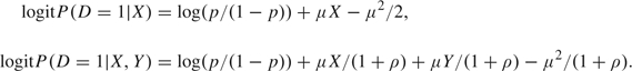Figure 1 displays pretest and posttest risks for 1000 observations. For the simulations, we choose the prevalence p = 0.2, correlation ρ = 0.1, 0.5, and 0.9, and μ = (1 + ρ)log(10) so that the covariate-adjusted odds ratio for Y is equal to 10 throughout. As expected, the distribution of logDLR_X(Y) is more concentrated about 0 when ρ is larger (Figure 1 panel (a)), and accordingly there is less spread of points about the 45^о line in the scatter plots (Figure 1 panel (b) through (d)).

Fig. 1.

Data simulated from a logistic regression model with normally distributed predictors (X,Y) that are correlated to varying degrees. Shown are the population distributions of covariate-specific logDLR_X(Y) in panel (a), and scatter plots of post- versus pretest risks in panel (b) ρ = 0.1, (c) ρ = 0.5, and (d) ρ = 0.9. High- and low-risk thresholds at 0.8 and 0.2 are displayed. In panel (a), the solid curve is the distribution of logDLR_X(Y) when ρ = 0.1, the dashed curve is for ρ = 0.5 and the dotted curve is for ρ = 0.9. In panels (b) through (d), solid circles indicate case observations and diamonds indicate controls.

To see the impact on risk reclassification, we choose thresholds of 0.2 and 0.8 to define low and high risk, respectively. Observe that when ρ is large, only a few subjects have risks that cross the thresholds by augmenting the predictor X to include Y. In contrast, when ρ is small, large numbers of subjects are reclassified as low, medium, and high risk. Interestingly, many risk reclassifications are in the “wrong direction,” with cases having lower risks and controls having higher risks after including Y in the risk calculation. This crucial point has been discussed previously by Pepe, Janes, and Gu (2007) and Janes and others (2008).

3. ESTIMATING THE COVARIATE-SPECIFIC DLR FUNCTION

For binary markers, Janssens and others (2005) proposed that logDLR_X(Y) could be estimated by fitting 2 logistic regression models, one to the pretest risk and one to the posttest risk:

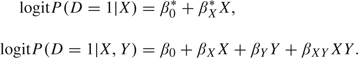For convenience, we write these as simple models in X and Y, but more general model forms could be employed. The covariate-specific DLR estimate is then given by the difference, which under these simple linear models is

This is clearly a valid approach for continuous markers too.

Observe that this approach to estimation accommodates case–control sampling. Only the intercept of the logistic model is affected by simple case–control designs, it is shifted by the factor logit(p) − logit(p_S), where p is the population prevalence and p_S is the sample prevalence of cases. Since logDLR_X(Y) involves the difference in the 2 intercepts, the adjustment factors cancel. A straightforward extension of this argument implies that case–control studies employing frequency matching with respect to baseline covariates are also accommodated by the methodology. Although both and cannot be estimated, their difference can.

Though coefficients in the DLR model can be directly estimated by fitting 2 logistic models and subtracting one from the other, it is not immediately clear how to make inference about the coefficients. Here, we adapt methods described by Pepe and others (1999). They consider simultaneously fitting multiple different regression models to the same outcome variable. They call the models “marginal with respect to covariates” to distinguish from the more familiar use of multiple models employing the same covariates but different outcome variables (Liang and Zeger, 1986), models that are “marginal with respect to outcome variables.” Estimating equations yield a sandwich variance–covariance matrix for coefficient estimates in the different models. Here, the common outcome variable is D and the method provides a variance–covariance matrix Σ_β for . It follows that the estimated variance–covariance matrix for the coefficients in the model for logDLR_X(Y) is given by , and the variance of can be estimated with , where

I denotes the (d + 1)×(d + 1) identity matrix, denotes a (d + 1)×(d + 1) matrix of zeros, and d is the dimension of X. Steps required to simultaneously fit 2 logistic regression models are detailed in Appendix A. In Tables 1 and 2, p-values for coefficients in the DLR models were obtained using this technique.

Table 1.

Baseline (pretest) and augmented (posttest) models for risk of hearing impairment based on a nested case–control substudy of the Neonatal Audiology for test B. Shown are log odds ratios for P(D = 1|X) and P(D = 1|X, Y) and coefficients for covariates in the corresponding model for logDLR_X(Y). Age is centered at 35 weeks. p-values in parentheses are calculated by comparing estimates with standard errors

Factor	Pretest risk	Posttest risk	log DLRX(Y)
Intercept	– 0.05 (0.67)	– 0.58 (< .001)	– 0.54 (1.00)
Age (weeks)	– 0.04 (0.04)	– 0.04 (0.05)	0.002 (0.27)
Location (booth versus room)	0.10 (0.49)	0.15 (0.34)	0.04 (0.72)
Age × location	0.07 (0.02)	0.07 (0.03)	– 0.005 (0.47)
Test result (Yes versus No)	—	1.06 (< 0.001)	1.06 (< 0.001)

Table 2.

Baseline model for risk of renal artery stenosis based on 426 patients and DLR model based on a nested case–control substudy of serum creatinine. Shown are log odds ratios for P(D = 1|X) and coefficients for covariates in the corresponding model for logDLR_X(Y). Continuous variables are standardized to mean 0 and variance 1. p-values in parentheses are calculated by comparing estimates with standard errors. Standard errors for coefficients in the logDLR model are calculated by adopting the techniques described in the appendix

Factor	Baseline risk	log DLRX(Y)	log DLRX(Y)∗
Intercept	– 2.54 (< .001)	0.06 (0.56)	0.07 (0.44)
Gender (female)	0.38 (0.18)	0.44 (0.01)	0.47 (0.01)
Age (per 10 years)	0.61 (< 0.001)	– 0.18 (0.002)	– 0.18 (0.003)
Hypertension	0.66 (0.03)	0.03 (0.81)	0.00
BMI (kg/m3)	– 0.20 (< 0.001)	0.03 (0.06)	0.03 (0.09)
Abdominal bruit	1.41 (< 0.001)	0.33 (0.15)	0.00
Atherosclerosis disease	0.91 (0.002)	– 0.45 (0.01)	– 0.42 (0.01)
log serum creatine	—	0.92 (< 0.001)	0.91 (< 0.001)

^*After setting to 0 coefficients for abdominal bruit and hypertension.

Note that if a factor enters into both logistic models with the same coefficient, it drops out of the DLR model. This indicates that the change in risk incurred by knowledge of Y does not depend on that factor. One can formally test hypotheses that elements of β_X − β_X^* are equal to 0 by comparing the regression coefficients in the DLR model with their estimated standard errors. A reduced model can then be fit to logDLR_X(Y) by forcing corresponding coefficients in the logistic models to be equal. Again, details are provided in Appendix A.

Here, we emphasize again the distinction between DLR_X(Y) and the covariate-adjusted effect of Y in the posttest risk model. Observe that only if β₀^* = β₀ and β_X^* = β_X, can one conclude that the covariate-adjusted effect of Y in the augmented model, P(D = 1|Y,X), is the same as the change in odds of disease incurred with knowledge of Y. The former is more relevant to etiologic research, while the latter is more relevant to diagnostic and prediction research.

One concern with fitting 2 logistic regression models to the same data is that the 2 models may not be compatible in the sense that their inherent relationship is ignored. An alternative approach is to fit a model to the posttest risk, P(D = 1|X,Y), and to the distribution of Y conditional on X, F(Y|X), and to calculate the pretest risk using the relationship

This has the advantage that F(Y|X) and P(D = 1|X,Y) are functionally independent. However, the approach is not only numerically more complicated but most importantly does not apply to case–control studies. We expect that by using sufficiently flexible models for pretest and posttest risk models and by using goodness-of-fit procedures for each model, issues with incompatibility will not arise.

4. COVARIATE EFFECTS ON A TEST FOR HEARING IMPAIRMENT

4.1. The study

The Neonatal Hearing Screening Study is a study of hearing screening in a cohort of high-risk newborn babies (Norton and others, 2000). Each baby in the study was tested in each ear with 3 passive hearing tests and evaluated with a gold standard behavioral test at 9–12 months of age. In the data set analyzed by Leisenring and others (1997), the tests are dichotomized and covariates include gestational age of the baby, location where the screening test was performed (hospital room or sound booth), and severity of hearing impairment for deaf ears. Here, we analyze the test labeled “B” in the publicly available data set, www.fhcrc.org/science/labs/pepe/dabs/. For simplicity, we restrict our analysis to the left ear only to avoid issues with correlations between ears. In total, 356 subjects have hearing impairment in the left ear. To illustrate our methodology, we simulate a nested case–control study from the cohort by selecting all 356 ears with hearing impairment and a random sample of 356 control ears with normal hearing.

4.2. The DLR of hearing test B

Overall in the population, test B has a true-positive rate, P(Y = 1|D = 1), of 61.5% and a false-positive rate, P(Y = 1|D = 0), of 37.3%. Therefore, its positive DLR, DLR(1), is TPR/FPR = 1.65, while its negative DLR, DLR(0), is (1 − TPR)/(1 − FPR) = 0.61. A clinician considering ordering test B for a child may give him a subjective probability p of being hearing impaired. If he were to order test B and it were positive, then according to (2.2) he would revise the probability to p⁺, where logit p⁺ = logit p + log1.65. For example, if p = 0.20, then a positive test would lead him to the revised probability p⁺ = 0.29. A negative test on the other hand would lead to the revised probability p⁻ = 0.13 since logit p + logDLR (0) = logit 0.2 + log0.61 = logit 0.13. Interventions for families with infants suspected of hearing impairment include counseling and education in regard to nonverbal communication skills. Potential drawbacks of intervention are the social consequences associated with labeling a child as hearing impaired. The clinician should only order the test if his recommendations about intervention will be different when his assessment of the child's chance of being hearing impaired is 0.29 or 0.13 versus when his assessment of the chance is the baseline value 0.20.

We next evaluate if the DLRs of the test vary with age of the child or location where the test is performed. That is, should the manner in which the physician uses the test result to update his assessment vary with these factors? Table 1 displays logistic models fit to the case–control study data. Both models fit the data well. Hosmer–Lemershow tests yielded a p-value of 0.31 for the pretest risk model and 0.72 for the posttest risk model. We see from Table 1 that gestational age of the child is associated with the child's risk of hearing impairment both in the absence and in the presence of knowledge of the test result. There is also a significant interaction between location and age in both pretest and posttest risk models. As expected, the newborn screening test result is strongly associated with risk of being hearing impaired. Interestingly, the coefficients associated with age and location factors in the pretest model are essentially unchanged when test result is added to the model. By subtraction, the coefficients associated with age and location in the logDLR model are therefore close to 0, and none are statistically significant. That is, the DLRs associated with the screening test result do not depend on the child's age or on location of testing. The clinician can therefore use the test result to update his assessments in the same manner regardless of the child's age or where the testing was done.

5. QUANTIFYING THE PERFORMANCE OF A MARKER

In this section, we are not interested in the covariate-specific DLR function for its own sake. Instead, we use it as a stepping stone toward evaluating the predictive impact of a continuous marker.

5.1. The renal artery stenosis study

In a study of 426 subjects undergoing renal arteriography reported by Janssens and others (2005), 98 (23%) were found to have significant stenosis. Baseline predictors of renal stenosis are shown in Table 2, along with logistic regression coefficients estimated using the entire set of 426 subjects. Continuous covariates, namely, age and BMI, are centered at their means, so that the baseline risk relates to a person of average age and BMI. All baseline covariates except gender are statistically significant risk factors.

We simulated a nested case–control marker study within this cohort by selecting all 98 cases and a random sample of 98 controls from the 328 controls in the cohort. We assume that the novel marker Y, serum creatinine, is only available for these patients. We analyzed serum creatinine on a logarithmic scale and standardized it to have mean 0 and standard deviation 1.

5.2. Results

We first show some key results pertaining to the incremental value of serum creatinine for risk prediction in this data set. Novel methods to arrive at these results will be described below. In Table 2 (column 2), coefficients of the log DLR model were obtained by subtracting coefficients of the pretest risk model from those of the posttest risk model. Both models were fit to the case–control subset. Hosmer–Lemershow tests yielded p-values of 0.16 and 0.92 for the pre- and posttest logistic regression models, indicating that both models fit the data well. Figure 2 displays scatter plots of pretest and posttest risks for the 98 cases and 98 controls in this study. We see that there is a slight tendency for posttest risks calculated for cases to increase relative to baseline (average change is 0.044), while risks decreased on average for controls (average change is 0.011). However, large changes in positive and negative directions are evident for both cases and controls. For illustration, suppose that a risk of 0.4 constitutes a high-risk threshold in the sense that if a subject has risk above 0.4 he is recommended for renal arteriography. We see from the margins of the scatter plots that in the absence of serum creatinine, 55% (95% confidence interval [CI] (0.43, 0.64)) of cases are classified as high risk and 5% (95% CI (0.01, 0.11)) of controls are classified as high risk. In the terminology of Pepe and others (2008), the true- and false-positive rates associated with the pretest risk model are 0.55 and 0.05, respectively. When serum creatinine is added to the model, the true-positive rate is increased from 55% to 62%. The false-positive rate is also increased slightly from 5% to 7%. Overall in the population, we estimate that 20% of patients are classified as high risk using a model that includes serum creatinine, while fewer, 17%, are classified as high risk in the absence of knowledge about their serum creatinine levels. Thus, by using serum creatinine to calculate risk, a larger number of high-risk individuals are identified, and importantly, a larger proportion of subjects with renal stenosis (cases) are recommended for the diagnostic procedure.

Fig. 2.

Scatter plots of risk estimates with and without serum creatinine as a predictor, for 98 cases and 98 controls in the renal stenosis substudy. For illustration, low- and high-risk thresholds of 0.1 and 0.4 are displayed. Panel (a) shows the pre- and posttest disease probabilities for cases, and panel (b) displays the probabilities for controls.

Now, consider a subject with baseline risk P(D = 1|X). Two specific examples are considered in Figure 3. The right panel concerns a man whose baseline risk is 0.27. The plots show estimates of the probability distributions of posttest risk for him. The bottom curves are cumulative distributions conditional on case or control status, while the upper curve shows the marginal distribution. Suppose his personal risk tolerance is high and he will opt for renal arteriography only if his risk of stenosis is 0.40 or more. We see that there is a 20% chance that after obtaining serum creatinine his posttest risk will be in this high-risk range. If he has renal stenosis, that chance is 37%, while it is only 16% if he does not in fact have renal stenosis. It appears that ascertainment of serum creatinine for him has a reasonable chance of affecting his decisions about undergoing renal arteriography.

Fig. 3.

Estimates of covariate-specific distributions of risk in the renal artery stenosis study. Shown are curves for 2 individuals. Left panel is for a 57-year-old female whose BMI is 26.77kg/m² and has hypertension but no atherosclerosis disease or abdominal bruit. Her baseline risk is 0.23. The right panel is for a 63-year-old male whose BMI is 30kg/m² and has hypertension and atherosclerosis disease but no abdominal bruit. His baseline risk is 0.27.

Suppose, however, that this subject has a low tolerance for risk and is inclined to opt for renal arteriography unless his calculated risk is below 10%. We see from Figure 3 that there is a very small chance, 0.04, that his posttest risk will be  < 10%, regardless of his true status. Therefore, there is no point in obtaining the marker for this subject. His risk calculated with serum creatinine will not lead to a different course of action from that calculated with the baseline factors only.

5.3. Methods

In this section, we describe methods to arrive at estimates of the posttest risks shown in Figure 2 and the individual posttest risk distribution curves shown in Figure 3 using covariate-specific estimates of the DLR function (Table 2).

Having fit a DLR regression model to the case–control data and a baseline risk model to the entire cohort, we use the relationship (2.2) to calculate from and (x_i) for each subject in the case–control subset. Posttest risk estimates are displayed in Figure 2. Empirical estimators of the marginal case and control posttest risk distributions follow. These are valid in an unmatched case–control study. Under a frequency-matched case–control design, the estimators would need to be weighted according to the population distributions of X in the case and control populations, which can be estimated from the parent cohort. The cumulative distribution of posttest risk in the population as a whole is the average of case and control posttest risk distributions, weighted according to the population prevalence which is 23% in our example. Sampling variability in the risk estimates is assessed with bootstrap resampling.

Now consider the estimated covariate-specific distributions of posttest risk shown in Figure 3, also known as covariate specific predictiveness curves (Huang and others, 2007). To calculate these, we model the distribution of Y as a function of X and case–control status using a semiparametric location scale model (Heagerty and Pepe, 1999):

where g is a specified function and the cumulative distribution of ϵ, denoted by F₀, is unspecified. The model is used in conjunction with the covariate-specific DLR_X(Y) function and the baseline risk, r(X), to calculate R_1,X(t) and R_0,X(t), the covariate-specific posttest risk distributions in cases and controls, respectively. In particular, let

then

The fitted DLR regression model and baseline risk value yield . The empirical distribution of residuals from the fitted model for Y gives rise to . The estimated covariate-specific marginal distribution of posttest risk is

In our analysis, we choose a linear link function g, and estimated coefficients are shown in Table 3. Sampling variability is assessed with the bootstrap.

Table 3.

Effects of baseline covariates and outcome on the marker distribution in the renal artery stenosis study

Factor	Coefficient (p-value)
Intercept	– 0.20 (0.08)
Gender (female)	– 0.58 (< 0.001)
Age (per 10 years)	0.17 (0.003)
Hypertension	– 0.07 (0.56)
BMI (kg/m2)	– 0.01 (0.29)
Abdominal bruit	– 0.18 (0.30)
Atherosclerosis disease	0.48 (0.001)
Renal artery stenosis	0.54 (< 0.001)

It is widely appreciated that the performance of a risk prediction model on the data used to fit the model can be optimistically biased. We used 10-fold cross-validation to reduce bias in estimates of the risks and their distributions. Results were almost identical. The results reported here did not employ cross-validation.

5.4. Risk thresholds and decisions to ascertain Y

Implicit in the above discussion is the existence of threshold values for risk that are used to make decisions, in this case for or against the renal arteriography procedure. Risk thresholds vary with the clinical context and may additionally vary among individuals. How to choose a risk threshold? The classic decision theoretic solution to choosing a risk threshold is fairly simple. Let C₀ (and B₀) denote the cost (and benefit) associated with being classified as high risk (and low risk) if the subject is in fact a control. Similarly, let B₁ (and C₁) denote the benefit (and cost) of being classified as high risk (and low risk) if the subject is a case. Then, the expected benefit of high-risk classification for a subject whose risk of being a case is given by r is rB₁ − (1 − r)C₀, where − C₀ is interpreted as a negative benefit. His expected benefit of low-risk classification is − rC₁ + (1 − r)B₀. The expected benefit with high-risk designation exceeds that of low-risk designation if r/(1 − r) > (B₀ + C₀)/(B₁ + C₁). In other words, he can expect to benefit from the high-risk designation if r > ℂ₀/(𝔹₁ + ℂ₀), where ℂ₀ = B₀ + C₀ is the net cost of high-risk classification for a control and 𝔹₁ = B₁ + C₁ is the net benefit for a case. The appropriate high-risk threshold is therefore ℂ₀/(𝔹₁ + ℂ₀), a direct function of the cost–benefit ratio, ℂ₀/𝔹₁. If a low-risk threshold is of interest, a similar exercise can be used to yield the value. In our example, the high-risk threshold of 0.4 corresponds to an implicit cost–benefit ratio of 2/3, while the cost–benefit ratio 1/9 corresponds to the risk threshold of 0.1.

Now, suppose a subject has baseline risk r(X) and high-risk threshold τ = ℂ₀/(𝔹₁ + ℂ₀). How should he formally decide to ascertain Y or not? Recall that if r(X) > τ, in the absence of Y he will choose to undergo the intervention associated with high-risk status and his expected benefit is r(X)B₁ − (1 − r(X))C₀. If he ascertains Y, the expected benefit is

(5.1)

assuming that the cost associated with ascertaining Y itself is negligible. The first and second components of (5.1) are the expected benefit for a case and a control, respectively. Observe that, by rearranging (5.1), it can also be represented as

The first and second components are counterparts of rB₁ − (1 − r)C₀ and − rC₁ + (1 − r)B₀, the expected benefit of high- and low-risk classification, but now each element is weighted by the corresponding probability of high- or low-risk designation conditional on case–control status.

By subtraction, we see that if r(X) > τ, he expects to gain more by ascertaining Y than not if

Equivalently when r(X) > τ, there is benefit to be expected by ascertaining Y and basing the decision on r(X,Y) if

A similar exercise indicates that when r(X) < τ, one should ascertain Y and base the decision on r(X,Y) if

In our illustration for the man with risk 0.27 on the basis of baseline factors (Figure 3, right panel), if his high-risk threshold is τ = 0.40, we found R_1,X(0.40) = 0.63 while R_0,X(0.40) = 0.84. Implicitly for this subject, ℂ₀/𝔹₁ = 2/3 as his choice of high-risk threshold is τ = 0.4. Since his baseline risk r(X) < τ, he should ascertain Y if

This condition holds. Therefore, he should ascertain Y and base his decision on r(X,Y) rather than on r(X). On the other hand, if his high-risk threshold is τ = 0.10, ℂ₀/𝔹₁ = 1/9 and we found R_1,X(0.10) = 0.05 and R_0,X(0.10) = 0. He should not ascertain Y since the condition

does not hold.

6. DISCUSSION

We have studied the DLR function in this paper, a measure of test performance that is popular in clinical medicine but is used in a simplified fashion in practice. We developed methods to make inference about the covariate-specific DLR function and demonstrated 2 uses for the methodology. First, we illustrated an investigation of covariate effects on DLR where the covariate effects themselves were of interest. Leisenring and Pepe (1998) provide another approach to DLR regression that applies only to dichotomous tests. Second, we showed how estimation of the covariate-specific DLR from a nested case–control study can allow us to evaluate the posttest risk distributions that can be obtained with a marker. Methods for making decisions about ascertainment of the marker follow.

We contrasted the covariate-specific DLR function with the covariate-adjusted association between outcome and test result. The former pertains more to diagnostic and prediction research than to etiologic research but is less familiar to biostatisticians. Since DLR_X(Y) is a function of Y, in and of itself it does not provide a simple summary of test performance when Y is continuous. One might consider standardizing marker values relative to their covariate-specific distributions in controls to make DLR_X(.) functions comparable across markers (Huang and Pepe, 2008) and across populations with different covariates. Development of sensible summary indices will be needed to formulate test statistics for comparing markers and subpopulations.

FUNDING

National Institute of Health (GM 54438 to M.P., CA 86368 to M.P. and W.G.).

Appendix A

A.1 An algorithm to simultaneously fit 2 logistic regression models

Suppose there are n subjects in the data set. Each subject has a record composed of disease status D, marker Y, and covariate vector X.

Write the 2 logistic regression models as

and

where V is a vector of covariates that are functions of (X,Y). Transformations and interactions as well as linear terms can be introduced in V.

1. Rearrange the data for each of the n subjects into 2 replicate records of the form (D_i,X_i,V_i), i = 1,…,n. The 2 records have the same outcome D_i and covariate vectors.

2. Define an indicator variable I_ij in the jth data record of the ith subjects with I_i1 = 1 and I_i2 = 0.

3. Define a vector with 4 components Z_ij = (1 − I_ij,(1 − I_ij)X_ij,I_ij,I_ijV_ij) for the jth record for subject i.

4. Fit a logistic regression model to D with predictor Z using the rearranged data. Generalized estimation equation methods are employed with independence as the working correlation structure.

5. A sandwich variance–covariance estimator for the regression coefficients is calculated that accounts for the fact that each subject contributes a pair of observations (cluster) to the analysis.

Note that in order to restrict the models so that coefficients associated with components of X are the same in the pretest and posttest risk models, one includes it as a single covariate X_ij rather than as 2 components (1 − I_ij)X_ij and I_ijh(X_ij) in step 3, where h(X_ij) indicates all terms related to X_ij in I_ijV_ij.

References

- Boyko EJ. Ruling out or ruling in disease with the most sensitive or specific diagnostic test: short cut or wrong turn? Medical Decision Making. 1994;14:175–179. doi: 10.1177/0272989X9401400210. [DOI] [PubMed] [Google Scholar]
- Bundy DG, Byerley JS, Liles EA, Perrin EM, Katznelson J, Rice HE. Does this child have appendicitis? Journal of the American Medical Association. 2007;298:438–451. doi: 10.1001/jama.298.4.438. [DOI] [PMC free article] [PubMed] [Google Scholar]
- Chen J, Pee D, Ayyagari R, Graubard B, Schairer C, Byrne C, Benichou J, Gail MH. Projecting absolute invasive breast cancer risk in white women with a model that includes mammographic density. Journal of the National Cancer Institute. 2006;98:1215–1226. doi: 10.1093/jnci/djj332. [DOI] [PubMed] [Google Scholar]
- Cook NR. Use and misuse of the receiver operating characteristic curve in risk prediction. Circulation. 2007;115:928–935. doi: 10.1161/CIRCULATIONAHA.106.672402. [DOI] [PubMed] [Google Scholar]
- Cook NR, Buring JE, Ridker PM. The effect of including C-reactive protein in cardiovascular risk prediction models for women. Annals of Internal Medicine. 2006;145:21–29. doi: 10.7326/0003-4819-145-1-200607040-00128. [DOI] [PubMed] [Google Scholar]
- Gail MH, Brinton LA, Byar DP, Corle DK, Green SB, Schairer C, Mulvihill JJ. Projecting individualized probabilities of developing breast cancer for white females who are being examined annually. Journal of the National Cancer Institute. 1989;81:1879–1886. doi: 10.1093/jnci/81.24.1879. [DOI] [PubMed] [Google Scholar]
- Giard RW, Hermans J. The evaluation and interpretation of cervical cytology: application of the likelihood ratio concept. Cytopathology. 1993;4:131–137. doi: 10.1111/j.1365-2303.1993.tb00078.x. [DOI] [PubMed] [Google Scholar]
- Goldman L, Cook EF, Mitchell N, Flatley M, Sherman H, Rosati R, Harrell F, Lee K, Cohn PF. Incremental value of the exercise test for diagnosing the presence or absence of coronary artery disease. Circulation. 1982;66:945–953. doi: 10.1161/01.cir.66.5.945. [DOI] [PubMed] [Google Scholar]
- Heagerty PJ, Pepe MS. Semiparametric estimation of regression quantiles with application to standardizing weight for height and age in US children. Applied Statistics. 1999;48:533–551. [Google Scholar]
- Huang Y, Pepe MS. Biomarker evaluation using the controls as a reference population. Biostatistics. 2008 doi: 10.1093/biostatistics/kxn029. (in press) [DOI] [PMC free article] [PubMed] [Google Scholar]
- Huang Y, Pepe MS, Feng Z. Evaluating the predictiveness of a continuous marker. Biometrics. 2007;63:1181–1188. doi: 10.1111/j.1541-0420.2007.00814.x. [DOI] [PMC free article] [PubMed] [Google Scholar]
- Janes H, Pepe MS, Gu W. Assessing the value of risk predictions using risk stratification tables. Annals of Internal Medicine. 2008 doi: 10.7326/0003-4819-149-10-200811180-00009. (in press) [DOI] [PMC free article] [PubMed] [Google Scholar]
- Janssens AC, Deng Y, Borsboom GJ, Eijkemans MJ, Habbema JD, Steyerberg EW. A new logistic regression approach for the evaluation of diagnostic test results. Medical Decision Making. 2005;25:168–177. doi: 10.1177/0272989X05275154. [DOI] [PubMed] [Google Scholar]
- Leisenring W, Pepe MS. Regression modelling of diagnostic likelihood ratios for the evaluation of medical diagnostic tests. Biometrics. 1998;54:444–452. [PubMed] [Google Scholar]
- Leisenring W, Pepe MS, Longton G. A marginal regression modelling framework for evaluating medical diagnostic tests. Statistics in Medicine. 1997;16:1263–1281. doi: 10.1002/(sici)1097-0258(19970615)16:11<1263::aid-sim550>3.0.co;2-m. [DOI] [PubMed] [Google Scholar]
- Liang KY, Zeger SL. Longitudinal data analysis using generalized linear models. Biometrika. 1986;73:13–22. [Google Scholar]
- Norton SJ, Gorga MP, Widen JE, Folsom RC, Sininger Y, Conewesson B, Vohr BR, Mascher K, Fletcher K. Identification of neonatal hearing impairment: evaluation of transient evoked otoacoustic emission, distortion product otoacoustic emission, and auditory brain stem response test performance. Ear and Hearing. 2000;21:508–528. doi: 10.1097/00003446-200010000-00013. [DOI] [PubMed] [Google Scholar]
- Pencina MJ, Dágostino RB, Sr, Dágostino RB, Jr, Vasan RS. Evaluating the added predictive ability of a new marker: from area under the ROC curve to reclassification and beyond. Statistics in Medicine. 2008;27:157–172. doi: 10.1002/sim.2929. [DOI] [PubMed] [Google Scholar]
- Pepe MS, Etzioni R, Feng Z, Potter JD, Thompson ML, Thornquist M, Winget M, Yasui Y. Phases of biomarker development for early detection of cancer. Journal of the National Cancer Institute. 2001;93:1054–1061. doi: 10.1093/jnci/93.14.1054. [DOI] [PubMed] [Google Scholar]
- Pepe MS, Feng Z, Gu JW. Commentary on ‘Evaluating the added predictive ability of a new marker: from area under the ROC curve to reclassification and beyond’. Statistics in Medicine. 2008;27:173–181. doi: 10.1002/sim.2991. [DOI] [PubMed] [Google Scholar]
- Pepe MS, Feng Z, Huang Y, Longton GM, Prentice R, Thompson IM, Zheng Y. Integrating the predictiveness of a marker with its performance as a classifier. American Journal of Epidemiology. 2008;167:362–368. doi: 10.1093/aje/kwm305. [DOI] [PMC free article] [PubMed] [Google Scholar]
- Pepe MS, Janes H, Gu W. in response to: Cook NR ‘Use and misuse of the receiver operating characteristic curve in risk prediction’. 2007. Letter to the Circulation. 116, e132. [DOI] [PubMed] [Google Scholar]
- Pepe MS, Janes H, Longton G, Leisenring W, Newcomb P. Limitations of the odds ratio in gauging the performance of a diagnostic, prognostic, or screening marker. American Journal of Epidemiology. 2004;159:882–890. doi: 10.1093/aje/kwh101. [DOI] [PubMed] [Google Scholar]
- Pepe MS, Whitaker RC, Seidel K. Estimating and comparing univariate associations with application to the prediction of adult obesity. Statistics in Medicine. 1999;18:163–173. doi: 10.1002/(sici)1097-0258(19990130)18:2<163::aid-sim11>3.0.co;2-f. [DOI] [PubMed] [Google Scholar]
- Thompson IM, Ankerst DP, Chi C, Goodman PJ, Tangen CM, Lucia MS, Feng Z, Parnes HL, Coltman CA. Screen-based prostate cancer risk: results from the prostate cancer prevention trial. Vol. 98. Journal of the National Cancer Institute; 2006. pp. 529–534. [DOI] [PubMed] [Google Scholar]
- Wang TJ, Gona P, Larson MG, Tofler GH, Levy D, Newton-Cheh C, Jacques PF, Rifai N, Selhub J, Robins SJ. Multiple biomarkers for the prediction of first major cardiovascular events and death. The New England Journal of Medicine. 2006;355:2631–2639. doi: 10.1056/NEJMoa055373. and others. [DOI] [PubMed] [Google Scholar]
- Wilson PW, Nam BH, Pencina M, Dágostino RB, Sr, Benjamin EJ, Odonnell CJ. C-Reactive protein and risk of cardiovascular disease in men and women from the Framingham Heart Study. Archives of Internal Medicine. 2005;165:2473–2478. doi: 10.1001/archinte.165.21.2473. [DOI] [PubMed] [Google Scholar]