StepBrothers: inferring partially shared ancestries among recombinant viral sequences

Abstract

Phylogeneticists have developed several statistical methods to infer recombination among molecular sequences that are evolutionarily related. Of these methods, Markov change-point models currently provide the most coherent framework. Yet, the Markov assumption is faulty in that the inferred relatedness of homologous sequences across regions divided by recombinant events is not independent, particularly for nonrecombinant sequences as they share the same history. To correct this limitation, we introduce a novel random tips (RT) model. The model springs from the idea that a recombinant sequence inherits its characters from an unknown number of ancestral full-length sequences, of which one only observes the incomplete portions. The RT model decomposes recombinant sequences into their ancestral portions and then augments each portion onto the data set as unique partially observed sequences. This data augmentation generates a random number of sequences related to each other through a single inferable tree with the same random number of tips. While intuitively pleasing, this single tree corrects the independence assumptions plaguing previous methods while permitting the detection of recombination. The single tree also allows for inference of the relative times of recombination events and generalizes to incorporate multiple recombinant sequences. This generalization answers important questions with which previous models struggle. For example, we demonstrate that a group of human immunodeficiency type 1 recombinant viruses from Argentina, previously thought to have the same recombinant history, actually consist of 2 groups: one, a clonal expansion of a reference sequence and another that predates the formation of the reference sequence. In another example, we demonstrate that 2 hepatitis B virus recombinant strains share similar splicing locations, suggesting a common descent of the 2 viruses. We implement and run both examples in a software package called StepBrothers, freely available to interested parties.

1. INTRODUCTION

The exchange of genetic information through homologous recombination substantially contributes to the diversity of life (Posada and others, 2002). Only recently recognized outside of sexually reproducing organisms (Temin, 1991), recombination is now expounded as a critical process in natural viral reproduction and pathogenesis (Rambaut and others, 2004). Two human viruses where recombination has clinical relevance are the human immunodeficiency virus 1 (HIV) and the hepatitis B virus (HBV). In several regions of the world, including Southeast Asia (Zhang and others, 2006) and Eastern Europe (Adojaan and others, 2006), recombinant strains of HIV dominate the acquired immunodeficiency syndrome epidemic. Similarly, recombinant strains of HBV have been found in Asia (Hannoun and others, 2000) and Africa (Owiredu and others, 2001).

To better appreciate the history, diversity, and ancestry of recombinant genomes, researchers have developed several approaches to infer recombination from molecular sequences of putative recombinants and representative parentals. In a recent simulation study comparing popular methods for recombination detection, Chan and others (2006) show that Bayesian phylogenetic-based methods have the best accuracy at detecting recombination events as well as recovering the point of recombination on simulated data. In addition, such likelihood-based methods allow for formal statistical inference on the recombination process. Other approaches that do not rely on formal statistical models are able to illuminate simple facts about the existence and properties of recombinants, but they provide results increasingly difficult to interpret, especially as hypotheses about recombination become more complex.

Bayesian phylogenetic-based methods fall into 2 separate forms. The first uses a hidden Markov model (HMM), where the hidden states are discrete phylogenetic topologies (Husmeier & McGuire, 2003); the second form uses Markov change-point (MCP) processes to model the spatial changes in the evolutionary history along the genome (Suchard and others, 2003), (Minin and others, 2005). Overall, the advantages of the MCP models outweigh the advantages of the HMM models. Chan and others (2006) show that the MCP models recover recombination events and the location of recombination break points better than the HMM models. Furthermore, the MCP models uniquely account for other forms of evolutionary process heterogeneity along the data, most importantly rate variation. Failure to account for such rate variation, particularly common in viruses, can lead to a high false-positive rate of recombination detection in real data (Dorman and others, 2002).

In spite of these advantages, MCP models assume that the topologies summarizing the phylogenetic relationship of sequences at any 2 alignment sites separated by a recombination break point are independent. Although this assumption may hold for recombinant sequences, it clearly does not for nonrecombinant sequences. To correct this poor assumption, we propose a more flexible framework for defining sequence relatedness across recombinant break points. This framework, deemed the random tips (RT) model, permits the inference of evolutionary histories where the number of tips on the phylogenetic tree is not fixed but is determined by the number of recombinants and break points in the data.

An illustration helps demonstrate how a fixed number of sequences can generate a random number of tips (Figure 1). The figure depicts the history of 3 sequences ℱ, 𝒢, and ℋ all sampled contemporaneously as they descend from a single common ancestor, sequence 𝒜. As shown, 𝒢 is a recombinant sequence; the left-hand portion of 𝒢 derives from sequence 𝒟, and the right-hand portion derives from sequence ℰ. At the time of recombination, both 𝒟 and ℰ were full length, but ℰ, the only contemporaneous record of these parental forms, retains information only from the leftmost portion of 𝒟 and the rightmost portion of ℰ. Assuming for the moment that we know 𝒢 is a recombinant, we split it into 2 separate sequences 𝒢₁ and 𝒢₂, such that 𝒢₁ contains the leftmost portion of 𝒟, 𝒢₂ the rightmost portion of ℰ, and both have missing information everywhere else. Sequences 𝒢₁ and 𝒢₂ represent our best current inference about the ancient sequences 𝒟 and ℰ. Once 𝒢 is split at the recombinant break point, we recover a bifurcating topology (right-hand side of Figure 1), where evidence of recombination is indicated by the fact that 𝒢₁ is most closely related to ℱ, but 𝒢₂ is most closely related to ℋThis strategy of data splitting or augmentation has several advantages. The strategy avoids the assumption of branch length and topological independence for sequences not sharing the selected break point. The use of a single phylogenetic tree maintains a time ordering on the evolutionary histories, allowing for the possibility of timing or at least bounding the time of recombination events. The ability to date recombinants is necessary to establish their role in epidemics and to tease apart the events giving rise to complex recombinants. The RT model naturally extends to the case of multiple recombinant sequences, permitting researchers to test if 2 or more recombinant sequences share a recombination event in time and sequence space.

Fig. 1.

Hypothetical evolutionary history relating recombinant sequence 𝒢 to its 2 parental sequences, ℱ and ℋ. Sequence 𝒜 is the ancestral sequence, and sequences ℱ, 𝒢, and ℋ are the sampled sequences. Since the first half of sequence 𝒢 derives from sequence 𝒟, while the second half of sequence 𝒢 derives from sequence ℰ, we split sequence 𝒢 into 2 separate sequences, 𝒢₁ and 𝒢₂. The blank portions of sequences 𝒢₁ and 𝒢₁ are missing data, coded as wild cards. Once the data set becomes augmented, we infer a phylogenetic tree on the 4 sequences.

A major difficultly with the RT model is the greatly expanded tree space. The space of all trees with a fixed number of tips is already extremely large, but the RT space contains all rooted bifurcating trees with a variable number of tips. Such a large space challenges prior specification. We overcome this issue by assuming a Yule-like branching process on the tree (Edwards, 1972). The other difficulty with the RT model springs from the sampling scheme required to make inference. Since the model space contains trees with a variable number of tips, we employ a reversible jump Markov chain Monte Carlo (MCMC) sampling scheme (Green, 1995).

We organize this paper as follows. Section 2 introduces the RT model, provides an example for clarity, and gives an outline of the MCMC scheme. In Section 3, we apply the RT model to both HIV and HBV data sets. Section 4 discusses the model's limitations and future directions for research. Extensive derivations are found in the supplementary material available at Biostatistics online (http://www.biostatistics.oxfordjournals.org.).

2. MODEL

The RT model uses a Bayesian phylogenetic framework. We develop the model likelihood and prior in the next 2 subsections and then turn to methods to draw inference under this model. For more background information on traditional phylogenetic modeling, we refer the reader to Felsenstein (2003).

2.1. Likelihood

Observed data Y^obs includes N aligned DNA or RNA sequences of length S. Each column Y_s^obs,s = 1,…,S, of Y^obs is a vector (Y_s1^obs,Y_s2^obs,…,Y_sN^obs)^′ such that each element Y_sn^obs corresponds to the molecular character at site s of sequence n, where n = 1,…,N. Allowable molecular characters include the standard 4 nucleotides {A, G, C, T/U}, wildcard characters, and gaps introduced into the alignment prior. We denote a wildcard by a *; it signifies the presence of a completely unobserved character. We order the sequences so that the first P sequences, 𝒫_p,p = 1,…,P, are the known nonrecombinant or possible parental sequences and the remaining R sequences, ℛ_r,r = 1,…,R, are the putative recombinant sequences, with P + R = N and P ≥ 2.

The decision whether to consider a specific sequence as a recombinant or parental ultimately relies upon the data. In our experience, investigators know or have defined specific strains as parental sequences. This occurs with both the HIV and the HBV data sets we examine. Of course, we do not believe that all data sets reflect such a nice distinction between parental and recombinant. For some bacterial data sets, nearly all sequences may demonstrate recombinant characteristics, an observation that limits the reach of the RT model. Still, these types of data reiterate that a statistician needs to tailor the model to the data, not the other way around.

We follow standard likelihood-based phylogenetic modeling and assume that sites are independent given the site-specific model parameters θ_s that characterize the evolutionary process (Felsenstein, 2003). We parameterize θ_s through a rooted bifurcating tree τ_s, a vector of bifurcation times T_s along τ_s, and a continuous-time Markov chain rate matrix Q_s. The matrix Q_s = {q_uv}_s,u,v∈{A, G, C, T/U}, provides the instantaneous transition rates for a continuous-time Markov process representing nucleotide substitution; Q_s follows the parameterization of Hasegawa and others (1985) that includes a site-specific rate multiplier μ_s, the ratio of the transition rate and the transversion rate κ_s, and the stationary distribution of the process π_s = (π_As,π_Gs,π_Cs,π_Ts). The finite-time transition matrix derives as P_s(x) = e^xQ_s = {p(u,v)|x}_s, such that {p(u,v)|x}_s is the probability that nucleotide u mutates into nucleotide v along a branch of length x. For identifiability between x and Q_s, we normalize Q_s so that μ_s is the expected number of substitutions along a branch of unit length 1. We set the stationary distribution π_s, at every site s, equal to the empirical nucleotide frequencies of the whole alignment (Li and others, 2000).

To avoid severe overfitting of the data, we employ a parsimonious Bayesian MCP approach (Suchard and others, 2003), (Minin and others, 2005). Rather than allowing each individual site s to have a distinct set of parameters θ_s, we assume 1 + R underlying MCP processes. The first MCP process describes the joint variation in the substitution process across all sequences. The remaining R processes partition the alignment into recombinant segments.

For the first MCP, we assume an unknown number J + 1 of nonoverlapping intervals such that κ_s and μ_s are the same for every site in a given interval. The intervals are partitioned at substitution change points ρ = (ρ₀,ρ₁,…,ρ_{J + 1}) such that 0 = ρ₀ < ρ₁ < ⋯ < ρ_{J + 1} = S + 1. Then for all sites s∈[ρ_{j − 1},ρ_j), κ_s = κ_j and μ_s = μ_j. We collect these parameters into vectors κ = (κ₁,κ₂,…,κ_{J + 1}) and μ = (μ₁,μ₂,…,μ_{J + 1}).

The specification of the other R MCP processes that determine τ_s and T_s is considerably trickier. We assume that for every recombinant sequence ℛ_r, there are an unknown number M_r + 1 nonoverlapping intervals and ξ_r corresponds to the vector of recombinant break points (ξ_r0,ξ_r1,…,ξ_{r,Mr + 1}), 0 = ξ_r0 < ξ_r1 < ⋯ < ξ_{r,Mr + 1} = S + 1. Following the illustration in Section 1, each of the intervals [ξ_{r,m − 1},ξ_rm),m = 1,…,M_r + 1, corresponds to a fragment of a partially observed sequence ℛ_rm. For sites s∈[ξ_{r,m − 1},ξ_rm), the nucleotide character of ℛ_rm at site s is the nucleotide character of ℛ_r at s. If s∉[ξ_{r,m − 1},ξ_rm), the character of ℛ_rm at site s is a *. We collect all the ξ_r into ξ = (ξ₁,ξ₂,…,ξ_R) and all the M_r into M = (M₁,M₂,…,M_R).

We can now construct τ and T. In this construction, we drop the subscript s since every site s has the same τ and T. Recombinant ℛ_r consists of M_r + 1 fragments; so across all recombinants there are a total of ∑_{r = 1}^RM_r + R = M partially unobserved sequences. Using these sequences, we create an augmented data set Y^aug with P + M total sequences. The first P sequences of Y^aug are 𝒫_p ordered according to p, and the next M are the partially observed sequences ℛ_r ordered first by r and then by m.

From the variable-sized Y^aug, we can naturally define τ as a rooted bifurcating tree with P + M external tips, such that each tip l_a corresponds to the ath sequence in Y^aug,a = 1,…,P + M. When a ≤ P, we refer to l_a as a parental tip and otherwise a recombinant tip. We label the root of τ as b₁ and its time of bifurcation t₁ as 1. The remaining internal bifurcation nodes b_i,i = 2,…,P + M − 1, are time ordered so that the times t_i of each b_i follow 1 = t₁ ≥ t₂ ≥ ⋯ ≥ t_{P + M − 1}. We define the parental tree to be that obtained from τ by removing all recombinant tips and corresponding b_i. We place all t_i in the vector T and require the distance from every l_a to b₁ to be 1. At a given site s, τ satisfies a molecular clock. Finally, due to identifiability problems with the likelihood, we restrict τ to lie in a subset of the space of all bifurcating trees with P + M tips; a point we return to in Section 2.4.

Using the definitions above, we set θ_s = (τ,T,κ_s,μ_s) and θ = (θ₁,…,θ_s). With this parameterization and the assumption of site independence, we write the likelihood as

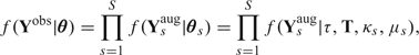(2.1)

where Y_s^aug is the sth column of Y^aug and f(Y_s^aug|τ,T,κ_s,μ_s) is the likelihood at site s, easily computed with the techniques in Felsenstein (1981).

We appreciate the complexity of the RT model notation; for clarity, Figure 2 summarizes the important quantities for a specific model realization. The figure assumes 2 parental sequences 𝒫₁ and 𝒫₂ and 2 recombinant sequences ℛ₁ and ℛ₂, all of length 300 in Y^obs. Sequence ℛ₁ has recombinant breaks at positions 100 and 200, and ℛ₂ has one recombinant break at position 200. A substitution change point is located at position 150; hence, M₁ = 2, M₂ = 1, J = 1, ρ = (0,150,301), ξ₁ = (0,100,200,301), and ξ₂ = (0,200,301).

Fig. 2.

Relationship between the observed data Y^obs, the augmented data Y^aug, and a phylogenetic tree τ with a random number of tips. Sequences 𝒫₁ and 𝒫₂ in Y^obs represent the parental sequences that do not split in the model. Sequences ℛ₁ and ℛ₂ represent the putative recombinant sequences, which can split. For the recombinant sequences in Y^aug, the black regions represent data from the corresponding full-length recombinant sequences in Y^obs, while the white regions represent wild cards (missing data). Each tip l_a on τ represents a sequence in Y^aug, and the b_i represents bifurcation points that occur at times t_i.

Corresponding to the substitution change point at site 150, there exists a κ₁, κ₂, μ₁, and μ₂, such that sites s∈[1,150) evolve according to κ₁ and μ₁ and the remaining sites evolve under κ₂ and μ₂.

Using Figure 2 as a guide, we see that transforming Y^obs into Y^aug generates 7 sequences: 𝒫₁, 𝒫₂, ℛ₁₁, ℛ₁₂, ℛ₁₃, ℛ₂₁, and ℛ₂₂. We now elaborate on the contents of a specific column, say 250, of Y^aug. For this column, Y₂₅₀^aug represents a vector of length 7, such that the characters in the first 2 positions come from the parental sequences, position 5 comes from ℛ₁, position 7 comes from ℛ₂, and the remaining positions are wildcards. All other sites in Figure 2 have a similar characterization.

2.2. Prior

We complete our model formulation by specifying a prior distribution over the evolutionary substitution change-point process (J,ρ,κ,μ) and the recombination break point processes (M,ξ) with corresponding (τ,T). The substitution change-point process finds a direct analog in Minin and others (2005). In brief, we assume that J follows a truncated Poisson distribution with prior expectation δ. Given J, the substitution change-point locations ρ are uniform over all possible unordered selections from S − 1 choices. The vectors (κ_j,μ_j) follow a standard hierarchical prior over ℝ² after suitable transformation with estimable location and scale parameters φ. The distributions for (κ_j,μ_j) are independent of each other given the hyperparameters φ (Minin and others, 2005), (Gelman, 2006).

The specification of (τ, T) and (M, ξ) differs substantially from that found in Minin and others (2005) and requires further discussion. Traditional Bayesian phylogenetic reconstruction grows from the premises of a fixed tree size. However, the RT model lives in a parameter space that grows with a variable number of tips. The space is also extremely large. Therefore, a noninformative prior over all trees places unreasonable mass on trees with unrealistically large numbers of recombination events.

As an alternative, we return to the roots of Bayesian phylogenetic inference (Rannala & Yang, 1996) and consider each tree as sprouting from a Yule process. The Yule process defines a pure birth branching process that is time homogeneous and begins with the first bifurcation event of a single particle into 2. At any time in the process, extant particles divide independently with infinitesimal-time probability λ. If one identifies the bifurcation points with the internal nodes b_i of τ, then the differences between branch lengths in T, e.g. t₅ − t₄ or t₆ − t₂, become exponential waiting times until division. Following Edwards (1972), for a given λ, the Yule process gives the joint probability density of a labeled, rooted bifurcating tree τ and branch length vector T, given V tips and t₁ = 1, as

(2.2)

We use this density as the joint prior of τ and T, where V = M + P. In this density, the parameter λ determines the tendency of branches to sprout closer to the sampling time, such that larger values of λ increase the tendency. Since we usually want branches to sprout uniformly over the tree a priori, we set λ = 0.05. However, in most standard phylogenetic problems, the posterior remains highly robust against larger values of λ since the likelihood dominates the prior.

The final pieces of the puzzle are the priors for M and ξ. We assume that M_r follows a truncated Poisson distribution with expectation η_r, η = (η₁,…,η_R). Since M jointly affects the probability of τ and T, the induced hierarchical prior on (M₁,M₂,…,M_R) generates a positive correlation on the M_r. For typical values of η, this correlation is usually small with values below 10%.

Given M, we assume a joint prior over ξ. While we could simply assume that each ξ_r is independently and identically distributed uniformly over M_i choices from S − 1 locations, this does not allow us to model the prior probability that 2 or more ℛ_r share the same break point. Also, with this independence prior, the prior probability that a recombinant break point coincides with 2 or more sequences is unrealistically small, usually less than 1%.

To correct these shortcomings, we develop an urn model that we first describe when R = 2. Assume that we have 2 urns with S − 1 labeled balls each of weight 1. The balls in the first urn represent locations in the sequence space of the first recombinant, while balls in the second urn represent the second recombinant. We select M₁ balls from the first urn and M₂ balls from the second urn and note the number of matching pairs O selected. We model the probability of the sample as , where w ≥ 0 and W is a normalizing constant. Physically, each of the M₁ + M₂ balls contributes 1 unit of weight to the sample; but, depending on w, the model adds extra “weight” to samples based on the number of shared pairs, more shared pairs imply a larger aggregate weight and a larger probability of occurrence. When w = 0, the model reduces to a product of independent priors, but as w grows large, the probability of at least one shared break point soon dominates the probability of none. For R recombinants, we model ξ as

(2.3)

where

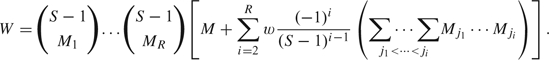(2.4)

We provide a derivation of W in the supplementary material available at Biostatistics online. The specification of O takes into account the size of an overlap break point: a break point that contains 3 separate sequences contributes 2 overlaps to O, 4 separate sequences contribute 3 overlaps to O, and so on. We take w as a known constant. In a setting similar to one in which our data live, setting w = 1000, S = 3224, R = 2, and η = (3.7,5.2) so that the E(M) = (3,4), the prior probability that at least 2 break points overlap is roughly 28%.

2.3. Posterior

The posterior distribution of the RT model falls out naturally using Bayes theorem. Specifically, if we let Θ define the collection of all model parameters, the posterior distribution of Θ given Y^obs is

(2.5)

To make inference on Θ, we employ an MCMC sampler that we describe in Section 2.5.

2.4. Identifiability issues

We restrict the tree τ to lie in a subspace of 𝒯, the set of all rooted bifurcating trees τ, where the number of tips of trees in 𝒯 can vary over a bounded set. The restrictions are necessary for 2 reasons. The space 𝒯 is potentially too large for efficient exploration because of the data augmentation procedure, and 𝒯 is not completely identifiable with respect to the data likelihood.

To manage the first difficulty, we assume that the topological relationships of the P parental sequences are known. Fixing the parental history remains reasonable for recombination inference involving distantly related parentals, such as those found in inter-subtype HIV and HBV evolution.

To appreciate the second restriction and its implications for data identifiability, we need to define a recombinant neighborhood 𝒩(l_a) for a tip l_a. Intuitively, 𝒩(l_a) is the collection of all recombinant tips on τ that share a common bifurcation point b_i with l_a. To be more precise, we establish a family of working sets related to l_a. We define the first working set to be ℋ₀ = ∅ or the empty set and the next working set to be ℋ₁ = {l_a}. Then, starting at l_a, we move upwards along τ toward b₁ and stop at the first bifurcation node b_i. The next working set ℋ₂ includes all the descendant tips of this b_i, note l_a∈ℋ₂. We continue this process of moving toward the root until we reach the root, at which point, we define our last working set and group all the working sets into ℋ = {ℋ₀,ℋ₁,ℋ₂,…}. Now, 𝒩(l_a) is the set with the largest cardinality in ℋ that does not include any parental tips. For any b_i, we also define 𝒩(b_i) in the same way, except now ℋ₁ includes all descendant nodes of b_i.

As an example, we illustrate the recombinant neighborhood definition on Figure 2. For tip l₃, ℋ = {∅,{l₃},{l₃,l₅},{l₃,l₅,l₇,l₂},{l₁,l₂,…,l₇}}, implying 𝒩(l₃) = {l₃,l₅}. Other examples include 𝒩(l₅) = {l₃,l₅}, 𝒩(b₃) = {l₃,l₅}, and 𝒩(l₁) = ∅.

Using the recombinant neighborhood definition, we can be precise about the identifiability issue. Let l_a and l_{a + 1} on τ correspond to one ℛ_r, and assume 𝒩(l_a) = 𝒩(l_{a + 1}). Since Y^aug is ordered by m, l_a corresponds to some ℛ_rm and l_{a + 1} corresponds to ℛ_{r,m + 1}. By the construction of ξ_r, ℛ_rm and ℛ_{r,m + 1} share a boundary ξ_rm. Now, from basic phylogenetic principles, if ℛ_rm and ℛ_{r,m + 1} are combined into a single sequence ℛ_rm^☆, and l_a (or l_{a + 1}) is removed from τ so that ℛ_rm^☆ corresponds to l_{a + 1} (or l_a) on τ^☆, the likelihood does not change.

In other words, the model can only identify the break ξ_rm if the 2 corresponding sequences on either side of ξ_rm do not have the same recombinant neighborhood. Or in more formal terms, if θ^☆ represents the likelihood parameters without ξ_rm, we have the situation where f(Y^obs|θ) = f(Y^obs|θ^☆) and θ≠θ^☆. Hence, a necessary condition that we impose for likelihood identifiability is that for all τ and all tips l_a and l_{a + 1} pertaining to the same ℛ_r, 𝒩(l_a)∩𝒩(l_{a + 1}) = ∅. This problem does not occur for tips such as l_a and l_{a + 2} because they are not adjacent in the sequence space.

The topology within each recombinant neighborhood is allowed to vary for 2 reasons. If tips from 2 or more recombinants are present in the same recombinant neighborhood, the topological structure within the neighborhood will affect the likelihood. Second, a change in the topology of the neighborhood can affect the prior through the sum of the branch lengths.

In addition to topological identifiability, changes in branch lengths within a recombinant neighborhood do not affect the data likelihood. However, the Yule-like tree prior influences these parameters, so the model posterior is identifiable, and importantly, we do not need to draw inferences about these heights. As an example, consider node b₃ and time t₃ in Figure 2. Due to the data augmentation, adjusting t₃ does not affect the data likelihood, but adjusting t₂ does. In later sections, we call nodes such as b₃ recombinant nodes and all others likelihood nodes to highlight about which node heights the data inform us.

2.5. Sampling

We employ a Metropolis-within-Gibbs MCMC sampler to gain samples from p(Θ|Y^obs). Because this sampler needs to move in the complicated parameter space of Θ, we implement a variety of transition kernels; details of which are found in the supplementary material available at Biostatistics online. Importantly, since the number of parameters in the model is unknown, we employ the reversible jump MCMC sampler of Green (1995). For more background information regarding MCMC for phylogenetic modeling, we refer the reader to Larget (2005).

We implement a working version of the sampler in Java called StepBrothers (available at http://www.biomath.ucla.edu/msuchard/StepBrothers/index.html). Before using this sampler to run examples, we have extensively checked our program by simulating from the prior distribution using the code and running numerous simulated examples. StepBrothers passed all tests. On the performance side, StepBrothers works well on moderately sized data sets but can bog down on data sets with large numbers of taxa. This performance issue, however, is not surprising. Via profiling, StepBrothers spends over 95% of its time calculating the likelihood: the bottleneck of all likelihood-based phylogeny inference. Therefore, on large data sets, users can face the same sorts of problems that plague likelihood-based phylogeny inference in general. To assess convergence of the MCMC sampler, we run multiple chains and assess the estimated posterior distributions. In the examples below, any differences between each chain can easily be attributed to Monte Carlo error.

3. DATA EXAMPLES

We demonstrate the benefits of the RT model on data from 2 sets of viral recombinants, one from HIV and the other from HBV. We show how the RT model permits analysis and comparison of multiple recombinants in order (1) to deduce whether they descend from the same recombinant ancestor or multiple distinct recombination events and (2) to date or at least bound the recombination events in time.

HIV circulating recombinant form 12 (CRF_12) affects patients in Argentina, Bolivia, Brazil, and Uruguay (Carr and others, 2001), (Quarleri and others, 2004). To better characterize the diversity and prevalence of CRF_12 in Argentina, Quarleri and others (2004) sample 284 recombinant HIV strains from patients seeking second-line antiretroviral therapy and sequence protease and the first 400 codons of reverse transcriptase from the pol region of HIV. The authors classify the 284 strains, along with the CRF_12 reference strain, and note the presence of 2 distinct subclades within the clade containing CRF_12. The authors are interested in whether the 2 subclades contain sequences with distinct recombination structure, but a dearth of appropriate modeling tools hamper their efforts.

Upon conducting a nationwide survey of HBV in China to better characterize the prevalence and diversity of the disease, Zeng and others (2005) identify genetic material from 8 patients who appear to descend from the D strain of HBV, but after more careful analysis, including full-genome sequencing, the authors discover that the 8 strains are recombinant HBV stains between HBV type C and type D (Wang and others, 2005). Our goal is to determine whether these strains share at least one recombination event in their histories.

3.1. Human immunodeficiency virus

We use the RT model to explore the relationship of recombinants in each subclade to the CRF_12 reference sequence (GenBank #AF385936). We select 2 patient sequences, 112567 (GenBank #AY365861) and 113314 (GenBank #AY365871), from the subclade containing CRF_12 and 1 sequence, 103520 (GenBank #AY365682), from the other. We use the same parental sequences as Quarleri and others (2004): A (GenBank #AF069671), B (GenBank #M17449), C (GenBank #AF110978), and F (GenBank #AF005494). We set the parental tree to be ((A, F), (B, C)). We treat the bifurcation times on τ as parameters that we infer, only the underlying parental tree topology remains fixed. We align the sequences first using an automated alignment program and then manually correct for obvious errors. Since the pol region of HIV is relatively conserved, we feel that the assumption of a fixed and known alignment has little impact on the results. For all analyses, we set w = 0 and η so that 0 break points occur with 50% prior probability.

We start off with separate, independent analyses to classify each recombinant sequence. As Figure 3(a) shows, sequences 112567, 113314, and CRF_12 have almost identical (F, B, F, B, F) recombinant structure. Sequence 103520, however, differs in 2 ways from CRF_12; the third break of 103520 occurs further right than the corresponding break in CRF_12, and sequence 103520 does not possess the fourth break present in CRF_12. A formal Bayes factor (BF) verifies this second observation: a recombinant break point is present in the interval (1400, 1497) for sequences 112567, 113314, and CRF_12 (BF  > 10⁵ for all 3), whereas there is little evidence to suggest that a break point exists in the same interval of sequence 103520 (BF ≈0.5).

We now compare each patient sequence to CRF_12. If a patient sequence and CRF_12 both descend from the same recombinant parent and have not experienced further recombination, then the 2 sequences should have the same recombinant neighborhoods throughout the genome. To summarize this information, we obtain the posterior probability that 2 sites, one from each of the recombinants, land on recombinant tips in the same neighborhood. If this occurs, we say these sites overlap on τ. We plot these posterior probabilities for all sites s in CRF_12 and sites s^′ in the patient sequences in Figures 3(a) and (b). We move the results for 112567 to Supplementary Figure SF-1, available at Biostatistics online, as they do not differ much from 113314. In these figures, the shade of the pixel (s,s^′) denotes the posterior probability of an overlap; the darker the shade, the more likely the 2 sites overlap and the more likely the 2 sites share their recombinant histories.

Fig. 3.

HIV recombinant analysis: (a) Posterior probabilities that each site in the alignment is a nearest neighbor to one of the parental nodes. The dashed line indicates the probability that a site phylogenetically arises from an F parental strain. The solid line indicates a B strain. (b) The probability that each site of the HIV patient sequence 113314 overlaps with each site of CRF_12. The shade of each pixel (s,s^′) represents the posterior probability that the 2 sites fall into the same recombinant neighborhood on τ. This figure shows 2 regions of high similarity between the patient sequence and the CRF_12. (c) In contrast, shows only one large of similarity between HIV patient sequence 103520 and CRF_12.

From Figure 3(b), we see that sequence 113314 shares 2 large areas of similarity with CRF_12. An analogous similarity exists between 112567 and CRF_12 in Supplementary Figure SF-1, available at Biostatistics online. In both cases, the dark regions present extremely strong evidence that the patient sequence derives from CRF_12. Through simulation, we find a 12% prior probability that any 2 sites overlap on τ. Thus, a 90% posterior probability in Figure 3(a) and Supplementary Figure SF-1, available at Biostatistics online, translates into a BF of 66. In Figure 3(b), we see that patient 103520 differs from the other 2; only one large area of similarity is shared with CRF_12.

Our final analysis in this section explores the timing of recombination. Since the RT model utilizes a single phylogenetic tree τ, a time ordering is maintained on τ, from which an upper bound on the time of recombination can be inferred for each break. Consider the first break in ℛ₁ in Figure 2. Here, the left portion of ℛ₁ corresponds to tip l₃ and the right portion corresponds to l₄. Noting this relationship, we see that tip l₃ diverges from τ_p at time t₂, while l₄ diverges at t₅. We focus on t₂ rather than t₃ since t₃ corresponds to a recombinant node, as defined in Section 2.4. With these 2 times, t₂ and t₅, we can infer an upper bound on the time of recombination by noting that the first recombination break point in ℛ₁ occurred before the min(t₂,t₅) = t₅.

Using the procedure just outlined, we consider such an upper bound as a proportion of the total tree height on each sequence using univariate analyses. To conduct this analysis, we use a different B parental (GenBank #AF156836) than Quarleri and others (2004) since their B parental was sampled approximately 14 years earlier than the other sequences in the data set. Because the topological space of our model can vary, we condition on the topological structure (F, B, F, B, F) for CRF_12, 112567, and 113314, and (F, B, F, B) for 103520. In Table 1, we present the upper bounds for all 4 breaks. We believe that the estimates from each analysis are comparable because the bifurcation time of the parental sequences A and F and the bifurcation time of the parental sequences B and C remain relatively constant in all 4 analyses (B–C difference < 0.04; A–F difference  < 0.01).

Table 1.

Expected upper bounds on the time of each recombinant break in the HIV example. The 4 breaks correspond to those at approximate positions 250, 350, 750, and 1450, as shown in Figure 3(a). Since no evidence exists for the fourth break in sequence 103520, we do not give a bound

	Break
Sequence	1	2	3	4
CRF_12	0.24	0.25	0.32	0.28
113314	0.20	0.21	0.29	0.27
112567	0.24	0.28	0.28	0.28
103520	0.38	0.38	0.39	NA

As shown in the table, the bounds for CRF_12, 113314, and 112567 generally group together. Sequence 103520, however, does not fit the pattern of the other 3 sequences; its bounds are relatively higher than the other 3. To gain a better handle on the results in Table 1, we roughly translate these proportions into actual dates. To do this, we follow Korber and others (2000) and use the year 1930 as the date of divergence for subgroup M in HIV-1. As the sequences in our data set were approximately sampled in the year 1998, we can translate the proportions into approximate dates using linear interpolation. With a little work, we see that the upper bound times for sequences CRF_12, 113314, and 112567 all fall around 1980 (1976–1984), while the upper bounds for sequence 103520 fall in the early 1970s (1971–1972).

The 95% posterior credible intervals corresponding to the estimates in Table 1 are all quite wide and overlap in all 4 sequences at all 4 breaks. For example, the RT model provides (0.03,0.33) as a credible interval for the first break in 113314. Therefore, we should not credit these differences as statistically significant. Still, the results do suggest another difference between the recombination histories of the 3 patient sequences.

As a whole, these results favor the hypothesis of differences between the recombination histories of 3 patient sequences. This implies that a discordance exists between the 2 subclades from Quarleri and others (2004). While not presented here, we conduct further analysis on additional sequences in each subclade. Even though it is difficult to generalize all the results, we find that sequences in the subclade containing CRF_12 tend to have 2 large areas of overlap with CRF_12 and 4 recombinant break points; the results are similar to the results from sequences 112567 and 113314. Sequences in the other subclade, however, have only 3 recombinant break points and 1 large area of overlap with CRF_12; the results are similar to those from 103520. Therefore, from our analyses, the 2 subclades found in Quarleri and others (2004) represent distinct recombination histories: one subclade shares its break points with CRF_12 and most likely represents an expansion of this variant across the population, while the second subclade exposes a unique pattern that apparently predates the formulation of CRF_12.

As with any statistical analysis, some issues remain with these results. In particular, the results in Figures 3(b) and (c) and Supplementary Figure SF-1, available at Biostatistics online, demonstrate 1 or 2 large areas of similarity with CRF_12, but the ambiguous results in the lower 2 areas beg for further explanation. Biologically, the results could simply imply that further recombination events occurred at the first 2 breaks. Other reasons include a lack of informative sites and violations of the strict molecular clock assumption across τ. These same issues can also affect the dating analysis, but we leave them for future research.

3.2. HBV recombinant

We now explore the relationship of 2 HBV sequences (GenBank #AF460143 and #AY817511), the later published in Wang and others (2005). For our analysis, we use 8 parental sequences: 3 D strains (GenBank #M32138, X02496, X72702), 3 C strains (GenBank #X02496, D12980, AB014381), 1 B strain (GenBank #D23677), and 1 A strain (GenBank #AF297623). We set η≈(3.7,5.2) so that E(M) = (3,4) and align the sequences in a similar method as the HIV example. All sequences are of length 3224.

While several features of the 2 sequences are comparable, we focus our attention on the location of the recombination break points within the 2 recombinant sequences. In particular, we conduct a BF test whether the 2 sequences share at least one recombinant break point. This hypothesis translates into whether the location of the break near position 1400 occurs at the same position in both sequences (Supplementary Figure SF-2, available at Biostatistics online). To carry out the test, we follow Suchard and others (2005) and estimate the BF under several values of overlap weight w. Estimating the BF across a wide spectrum of weights w allows us to obtain a more accurate estimate of the BF, gain insight into the joint prior over ξ, and expose possible programing errors. After performing MCMC simulations at 8 values of w ranging from 20 to 10 000, we estimate the BF = 5.3 (Supplementary Figure SF-3, available at Biostatistics online). While not providing overwhelming support for our hypothesis, this BF does suggest the sharing of at least one break point.

4. DISCUSSION

The RT model presented in this paper fosters clear advantages over previous methodologies. With its more appropriate assumptions regarding the recombination history, the RT model allows researchers to bound times of recombination and infer relationships between multiple recombinant sequences. Without these 2 new forms of data analysis, we would not have discovered the discordant recombination histories in Section 3.1.

A few aspects of the RT model deserve more attention. The RT model relies upon a strict molecular clock assumption: the substitution rate μ along τ remains constant. In some data situations, strong evidence exists that μ changes along τ as time progresses. In these situations, assumption of a constant rate can lead to incorrect topology estimation (Ho & Jermiin, 2004). For these reasons, we plan to explore alternatives to a strict molecular clock for the RT model. Such alternatives include the relaxed clock model of Drummond and others (2006), but issues arise with model identifiability.

Beyond the molecular clock assumption, the RT model also requires at least 2 parental sequences to be present in the data. For intrahost sequences from rapidly evolving viruses, this requirement may not hold because a substantial minority of the sequences present in the data may be recombinants. To handle this more extreme case, a new technique for phylogenetic-based recombination detection exploiting ancestral recombination graphs (ARGs) may afford a future solution. First developed by Hudson (1983), Hudson (1990) and later by Griffiths & Marjoram (1996), an ARG is a graph much like a phylogenetic tree but allows for the complete characterization of the recombination history for all sequences present within the data. The ARG's benefits include the removal of the a priori distinction between parental sequences and recombinant sequences. Also, ARGs naturally generalize and extend the RT framework presented in this paper. By simply constraining certain sequences from recombining in an ARG, we can find a surjective function from ARG space to RT tree space. We further elaborate on this function in Supplementary Figure SF-4, available at Biostatistics online. Even so, for the ARG, the sequence data contain no more information about the recombination times than the bounds provided by the RT model. So, until sampling methods for ARGs advance to match the field's successes with trees, we endorse the use of random-tipped trees.

FUNDING

National Institutes of Health (AI07370 to E.W.B., GM068955 to K.S.D. and M.A.S.).

References

- Adojaan M, kivisild T, Männik A, Onu krispin T, Ustina V, Zilmer k, Liebert E, Jaroslav N, Priimägi L, Tefanova V. Predominance of a rare type of HIV-1 in Estonia. Journal of Acquired Immune Deficiency Syndromes. 2006;39:598–605. and others. [PubMed] [Google Scholar]
- Carr J, Avila M, Carrillo MG, Salomon H, Hierholzer J, Watanaveeradej V, Pando M, Negrete M, Russell K, Sanchez J. Diverse BF recombinants have spread widely since the introduction of HIV-1 into South America. AIDS. 2001;15:F41–F47. doi: 10.1097/00002030-200110190-00002. and others. [DOI] [PubMed] [Google Scholar]
- Chan C, Beiko R, Ragan M. Detecting recombination in evolving nucleotide sequences. BMC Bioinformatics. 2006;7:412–426. doi: 10.1186/1471-2105-7-412. [DOI] [PMC free article] [PubMed] [Google Scholar]
- Dorman K, Kaplan A, Sinsheimer J. Bootstrap confidence intervals for HIV-1 recombinants. Journal of Molecular Evolution. 2002;54:200–209. doi: 10.1007/s00239-001-0002-4. [DOI] [PubMed] [Google Scholar]
- Drummond A, Ho S, Phillips M, Rambaut A. Relaxed phylogenetics and dating with confidence. PLoS Biology. 2006;4:699–710. doi: 10.1371/journal.pbio.0040088. [DOI] [PMC free article] [PubMed] [Google Scholar]
- Edwards A. Estimation of the branch points of a branching diffusion process. Journal of the Royal Statistical Society, Series B (Methodological) 1972;32:155–174. [Google Scholar]
- Felsenstein J. Evolutionary trees from DNA sequences: a maximum likelihood approach. Journal of Molecular Evolution. 1981;17:368–376. doi: 10.1007/BF01734359. [DOI] [PubMed] [Google Scholar]
- Felsenstein J. Inferring Phylogenies. Sunderland, MA: Sinauer Associates; 2003. [Google Scholar]
- Gelman A. Prior distributions for variance parameters in hierarchical models. Bayesian Analysis. 2006;1:515–534. [Google Scholar]
- Green P. Reversible jump Markov chain Monte Carlo computation and Bayesian model determination. Biometrika. 1995;82:711–732. [Google Scholar]
- Griffiths R, Marjoram P. Ancestral inference from samples of DNA sequences with recombination. Journal of Computational Biology. 1996;3:479–502. doi: 10.1089/cmb.1996.3.479. [DOI] [PubMed] [Google Scholar]
- Hannoun C, Norder H, Lindh M. An aberrant genotype revealed in recombinant hepatitis B virus strains from Vietnam. Journal of General Virology. 2000;81:2267–2272. doi: 10.1099/0022-1317-81-9-2267. [DOI] [PubMed] [Google Scholar]
- Hasegawa M, Kishino H, Yano T. Dating the human-ape splitting by a molecular clock of mitochondrial DNA. Journal of Molecular Evolution. 1985;22:160–174. doi: 10.1007/BF02101694. [DOI] [PubMed] [Google Scholar]
- Ho S, Jermiin L. Tracing the decay of the historical signal in biological sequence data. Systematic Biology. 2004;53:628–637. doi: 10.1080/10635150490503035. [DOI] [PubMed] [Google Scholar]
- Hudson R. Properties of a neutral allele model with intragenic recombination. Theoretical Population Biology. 1983;23:183–201. doi: 10.1016/0040-5809(83)90013-8. [DOI] [PubMed] [Google Scholar]
- Hudson R. Gene genealogies and the coalescent process. In: Futuyma D, Antonovics J, editors. Oxford Surveys in Evolutionary Biology. Volume 7. New York: Oxford University Press; 1990. pp. 1–44. [Google Scholar]
- Husmeier D, McGuire G. Detecting recombination in 4-taxa DNA sequence alignments with Bayesian hidden Markov models and Markov chain Monte Carlo. Molecular Biology and Evolution. 2003;20:315–337. doi: 10.1093/molbev/msg039. [DOI] [PubMed] [Google Scholar]
- Korber B, Muldoon M, Theiler J, Gao F, Gupta R, Lapedes A, Hahn B, Wolinsky S, Bhattacharya T. Timing the ancestor of the HIV-1 pandemic strains. Science. 2000;288:1789–1796. doi: 10.1126/science.288.5472.1789. [DOI] [PubMed] [Google Scholar]
- Larget B. Introduction to Markov chain Monte Carlo methods in molecular evolution. In: Nielsen R, editor. Statistical Methods in Molecular Evolution. New York: Springer; 2005. pp. 45–62. [Google Scholar]
- Li S, Pearl D, Doss H. Phylogenetic tree construction using Markov chain Monte Carlo. Journal of the American Statistical Association. 2000;95:493–508. [Google Scholar]
- Minin V, Dorman K, Fang F, Suchard M. Dual multiple change-point model leads to more accurate recombination detection. Bioinformatics. 2005;21:3034–3042. doi: 10.1093/bioinformatics/bti459. [DOI] [PubMed] [Google Scholar]
- Owiredu W, Kramvis A, Kew M. Molecular analysis of hepatitis B virus genomes isolated from black african patients with fulminant hepatitis B. Journal of Medical Virology. 2001;65:485–492. [PubMed] [Google Scholar]
- Posada D, Crandall K, Holmes E. Recombination in evolutionary genomics. Annual Reviews of Genetics. 2002;36:75–97. doi: 10.1146/annurev.genet.36.040202.111115. [DOI] [PubMed] [Google Scholar]
- Quarleri J, Rubio A, Carobene M, Turk G, Vignoles M, Harrigan R, Montaner J, Salomon H, Carrillo MG. HIV Type 1 BF recombinant strains exhibit different pol gene mosaic patterns: descriptive analysis from 284 patients under treatment failure. AIDS Research and Human Retroviruses. 2004;20:1100–1107. doi: 10.1089/aid.2004.20.1100. [DOI] [PubMed] [Google Scholar]
- Rambaut A, Posada D, Crandall K, Holmes E. The causes and consequences of HIV evolution. Nature Reviews Genetics. 2004;5:52–61. doi: 10.1038/nrg1246. [DOI] [PubMed] [Google Scholar]
- Rannala B, Yang Z. Probability distribution of molecular evolutionary trees: a new method of phylogenetic inference. Journal of Molecular Evolution. 1996;43:304–311. doi: 10.1007/BF02338839. [DOI] [PubMed] [Google Scholar]
- Suchard M, Weiss R, Dorman K, Sinsheimer J. Inferring spatial phylogenetic variation along nucleotide sequences: a multiple changepoint model. Journal of the American Statistical Association. 2003;98:427–437. [Google Scholar]
- Suchard M, Weiss R, Sinsheimer J. Models for estimating Bayes factors with applications to phylogeny and tests of monophyly. Biometrics. 2005;61:665–673. doi: 10.1111/j.1541-0420.2005.00352.x. [DOI] [PubMed] [Google Scholar]
- Temin H. Sex and recombination in retroviruses. Trends in Genetics. 1991;7:71–74. doi: 10.1016/0168-9525(91)90272-R. [DOI] [PubMed] [Google Scholar]
- Wang Z, Liu Z, Zeng G, Wen S, Qi Y, Ma S, Naoumov N, Hou J. A new intertype recombinant between genotypes C and D of hepatitis B virus identified in China. Journal of General Virology. 2005;86:985–990. doi: 10.1099/vir.0.80771-0. [DOI] [PubMed] [Google Scholar]
- Zeng G, Wang Z, Wen S, Jiang J, Wang L, Cheng J, Tan D, Xiao F, Ma S, Li W. Geographic distribution, virologic and clinical characteristics of hepatitis B virus genotypes in China. Journal of Viral Hepatitis. 2005;12:609–617. doi: 10.1111/j.1365-2893.2005.00657.x. and others. [DOI] [PubMed] [Google Scholar]
- Zhang Y, Lu L, Ba L, Yang L, Jia M, Wang H, Fang Q, Shi Y, Yang W, Chang G. Dominance of HIV-1 subtype CRF_AE in sexually acquired cases leads to a new epidemic in Yunnan Province of China. PLoS Medicine. 2006;3:2065–2076. doi: 10.1371/journal.pmed.0030443. and others. [DOI] [PMC free article] [PubMed] [Google Scholar]
Associated Data
This section collects any data citations, data availability statements, or supplementary materials included in this article.