Graph-partitioned spatial priors for functional magnetic resonance images

Abstract

Spatial models of functional magnetic resonance imaging (fMRI) data allow one to estimate the spatial smoothness of general linear model (GLM) parameters and eschew pre-process smoothing of data entailed by conventional mass-univariate analyses. Recently diffusion-based spatial priors (Harrison et al., 2008) were proposed, which provide a way to formulate an adaptive spatial basis, where the diffusion kernel of a weighted graph-Laplacian (WGL) is used as the prior covariance matrix over GLM parameters. An advantage of these is that they can be used to relax the assumption of isotropy and stationarity implicit in smoothing data with a fixed Gaussian kernel. The limitation of diffusion-based models is purely computational, due to the large number of voxels in a brain volume. One solution is to partition a brain volume into slices, using a spatial model for each slice. This reduces computational burden by approximating the full WGL with a block diagonal form, where each block can be analysed separately. While fMRI data are collected in slices, the functional structures exhibiting spatial coherence and continuity are generally three-dimensional, calling for a more informed partition. We address this using the graph-Laplacian to divide a brain volume into sub-graphs, whose shape can be arbitrary. Their shape depends crucially on edge weights of the graph, which can be based on the Euclidean distance between voxels (isotropic) or on GLM parameters (anisotropic) encoding functional responses. The result is an approximation the full WGL that retains its 3D form and also has potential for parallelism. We applied the method to high-resolution (1mm³) fMRI data and compared models where a volume was divided into either slices or graph-partitions. Models were optimized using Expectation-Maximization and the approximate log-evidence computed to compare these different ways to partition a spatial prior. The real high-resolution fMRI data presented here had greatest evidence for the graph partitioned anisotropic model, which was best able to preserve fine functional detail.

Introduction

Functional magnetic resonance imaging (fMRI) data are typically smoothed using a fixed Gaussian kernel before mass-univariate estimation of general linear model (GLM) parameters (Friston et al., 2006), referred to hereafter as parameters. An alternative is to include smoothness as a hyperparameter of a multivariate statistical model that encodes similarity between neighbouring voxels (Flandin and Penny, 2007; Gossl et al., 2001; Penny et al., 2005; Woolrich et al., 2004). These Bayesian spatial models estimate the smoothness of each parameter image in an optimal way and do not require data to be smoothed prior to entering a statistical model. An additional advantage is that the evidence for different spatial models (i.e., priors) can be compared (MacKay, 2003). However, there are two key issues with spatial models for fMRI data; (i) given the convoluted structure of the cortex and patchy functional segregation, the smoothness of a parameter image, in general, varies over anatomical space in a non-stationary fashion, i.e. realistic spatial models are required and (ii) the inversion (i.e., parameter estimation, given data) of such models is computationally demanding, due to the large number of voxels in a brain volume.

A solution to (i) has been proposed that uses diffusion-based spatial priors (Harrison et al., 2008). An advantage of using a diffusion kernel, i.e. matrix exponential of a scaled graph-Laplacian (Chung, 1997), as the covariance compared to the Laplacian as a precision matrix (i.e. a Laplacian prior, used for example in Penny et al, 2005), is that its spatial extent can be optimized. The scale (hyper)-parameter, τ, of the diffusion kernel, K₂ = exp(−Lτ), plays an important role in that its value determines whether the kernel encodes local (i.e. nearest neighbour coupling in the graph-Laplacian, L) or global properties (i.e. eigenvectors of L) of the graph. For small values of τ this is best seen using a first order Taylor expansion of the matrix exponential, K₂ ≈ I − Lτ. However, as τ increases the kernel becomes dominated by lower spatial frequency eigenmodes. Using the eigensystem of the graph-Laplacian to compute the matrix exponential also means that we have an explicit spatial basis set of the prior covariance. This again is in contrast to Laplacian priors, where the spatial basis is implicit. In addition, Penny et al factorize the posterior density of GLM parameters over voxels, thereby avoiding inversion of the Laplacian matrix. This means that the spatial prior encodes local and not global properties of the graph. The downside of being able to optimize the spatial scale of the kernel is that it requires computing the reduced eigensystem of the graph-Laplacian, which has limited its application to one or two slices. The posterior density could also be factorised over voxels, however, the bottleneck is still computing this reduced eigensystem.

A way to facilitate this is to divide a volume into slices (similar to Flandin and Penny, 2007) and thereby reduce the Laplacian matrix to block-diagonal form. The issue with this is that the 3D prior has been reduced to a set of 2D priors. Our proposal is to use the graph-Laplacian to partition a volume into 3D segments, which provides an alternative that retains the 3D nature of the spatial prior and the computational advantage of a block-diagonal form. The eigensystem of each block can then be computed easily using standard Matlab routines. Note that this is a pragmatic approach to the problem, which does not seek to segment a brain volume into spatially distributed causes; however, its advantages include potential for parallelism and extension to include overlap among segments, i.e. soft instead of hard partition boundaries (see discussion). We first consider the more general problem of image segmentation before specific graph-partitioning algorithms.

Image segmentation algorithms (Aubert and Kornprobst, 2002) have been developed for use in, for example, computer vision (Shapiro and Stockman, 2001) and medical imaging (Pham et al., 2000). Many methods are available e.g. based on decomposing an image into approximately piece-wise constant regions and a set of edges (Mumford and Shah, 1989), level sets (Osher and Paragios, 2003) and graph partitioning (Grady, 2006; Grady and Schwartz, 2006; Qui and Hancock, 2007; Shi and Malik, 2000). The focus of this paper will be the latter, in particular, on methods that use the Laplacian matrix also called the graph-Laplacian, which is our preferred rhetoric. Applications to MRI data include spatial mixture models using Gaussian Markov random fields (Held et al., 1997; Wells et al., 1996; Woolrich and Behrens, 2006; Zhang et al., 2001) and clustering techniques (Flandin et al., 2002; Thirion et al., 2006). Graph-Laplacians have been used to segment structural MRI data (Liang et al., 2007; Song et al., 2006; Tolliver et al., 2005) and anatomo-functional parcellation (Flandin et al., 2002; Thirion et al., 2006) proposed to partition fMRI data into many small, homogeneous regions, or parcels, which employs clustering algorithms such as Gaussian mixture models (Penny and Friston, 2003) or spectral clustering (Tenenbaum et al., 2000). This latter approach is a convenient way to reduce the dimensionality of a brain volume and has been used to perform random effects (i.e. between subjects) analysis of fMRI data. The approach we propose is different in that each segment is not assumed to be homogeneous and is modelled using a multivariate spatial model to provide optimised parameter estimates for every voxel in every segment.

The basic idea is to represent a brain volume as an irregular graph that is defined by vertex (node) and weighted edge sets. Vertices correspond to voxels and edges are defined by specifying neighbours to each vertex. Weights can then be placed on the edges and the graph represented by a graph-Laplacian. The vertex set, or brain volume of voxels, can be defined using a mask, e.g. based on an anatomical atlas to define a volume of interest or computed from tissue probability maps (Ashburner and Friston, 2005) to exclude voxels in regions containing cerebral spinal fluid. In general, this leads to an irregular graph, in that it has irregular boundaries, i.e. is not a box. The advantage here is that a spatial model can be used to analysis a volume of interest; however, computing with irregular graphs is more computationally demanding than regular. Note that white matter could also be excluded or indeed one could limit the nodes to a cortical mesh (see discussion). The eigensystem of a graph-Laplacian can be used to compute the diffusion kernel, which for large graphs, is computationally demanding. A way to deal with this is to reduce it to block-diagonal form, which can be achieved using graph-partitioning algorithms. Given a 3D graph, each block or segment¹ will be, in general, a 3D sub-volume, which can be used to provide a piecewise spatial prior of brain data.

Finding an optimal partition of a graph, in terms of computational complexity, is an NP-hard (nondeterministic polynomial-time hard) problem; i.e., it is at least as hard as the hardest problems in NP (Garey and Johnson, 1979). As such many heuristics have been formulated. Examples of publicly available software packages are Chaco (Hendrickson and Leland, 1994), Metis (Karypis and Kumar, 1998), Meshpart (Gilbert et al., 1998) and Graph Analysis Toolbox (Grady and Schwartz, 2003). Many of these methods use the graph-Laplacian. The challenge is to define a function over a graph, which can be used to divide the vertex set into two subsets that share a minimal number of edges. In particular, spectral graph partitioning (Chung, 1997; Shi and Malik, 2000) uses the second eigenvector (Fiedler vector) of the graph-Laplacian to achieve this. That is, it uses global features of the graph to partition it into segments. This can be repeated for each segment, in a recursive scheme. An alternative, that also uses the graph-Laplacian, is the isoperimetric method. This uses the solution of a linear system of equations instead of an eigenvalue problem, which leads to improved speed and numerical stability (Grady and Schwartz, 2006). The solution is a function over the graph that can be used recursively, as with spectral partitioning.

The edge weights of a graph-Laplacian play a crucial role in determining the shape of segments. If they depend on Euclidean distance between voxels, then segments depend on the overall shape of the graph. An alternative, used to partition general images (Grady and Schwartz, 2006; Qui and Hancock, 2007) is to make weights a function of pixel values. This means that not only the shape of the image is encoded in the graph, but also the topology, i.e. connectivity, of its pixel values. The result is segmentation that respects boundaries between pixel values; i.e. partition boundaries tend to be along lines of steepest spatial gradient (edges of an image). This idea can be translated to partition a spatial prior of fMRI data by making edge weights depend on the values of a GLM parameter image that encodes functional activations. This leads to a functionally-informed block-wise approximation of the full graph-Laplacian, where in general, a volume is cut along boundaries between functionally specific regions.

This paper is organized as follows; the first section reviews a diffusion-based spatial model used to analysis fMRI data. We summarise the steps involved in this approach; however, full details can be found in (Harrison et al., 2008). We then consider the formulation of the graph-Laplacian from vertex and edge sets. In particular, we focus on computing edge weights that depend on ordinary least square (OLS) parameter estimates of non-smoothed data, which leads to an anisotropic (i.e., encoding a preferred direction) graph-Laplacian. Without this dependence it is isotropic. This is followed by an outline of the partitioning algorithm (full details can be found in Grady and Schwartz, 2006) for which we provide an intuitive illustration using a synthetic image. In the results section, we demonstrate the approach using a volume of synthetic fMRI data before applying it to high-resolution fMRI (hr-fMRI) data acquired during visual processing. Note that a surface based analysis could also be performed on these data, however, the focus of this current work is volume data, in particular, comparing analyses based on dividing a volume into slices or a graph partition (see discussion). We conclude by discussing some issues with the current implementation and comment on future developments.

Method

Diffusion-based models depend on the inversion of a N_V × N_V covariance matrix, which is the same in general for Gaussian process models, wherein the computational challenge lies. We therefore proceed in three steps; (1) define a volume using a mask, which allows for an informed selection of voxels, (2) partition this volume into computationally manageable segments (which in this paper contained ~ 1– 2×10³ voxels) and (3) optimize a spatial model for each segment separately.

Our main aim here is to describe the second of these steps, which we do after providing an outline of the third. First, we describe the spatial GLM used to analyse a segment of fMRI data, which uses a hierarchical (i.e., empirical Bayes) two-level model, where the second level contains a spatial prior over parameter values at the first level. We then provide details of how to define a graph-Laplacian over a brain volume and use it to partition the volume recursively into segments.

Spatial priors for fMRI

In this section, we outline a two-level GLM in terms of matrix-variate normal densities (Gupta and Nagar, 2000). We start with a linear model, under Gaussian assumptions, of the form

$$\begin{array}{c}Y=X\beta +{\epsilon }_1\hfill \\ \beta ={\epsilon }_2\hfill \\ {\epsilon }_i~N_{r_i,c_i}(0,S_i\otimes K_i)\hfill \end{array}\Rightarrow \begin{array}{c}\hfill p(Y,\beta \mid X)=p(Y\mid X,\beta )p\left(\beta \right)\hfill \\ \hfill p(Y\mid X,\beta )=N_{r_1,c_1}(X\beta ,S_1\otimes K_1)\hfill \\ \hfill p\left(\beta \right)=N_{r_2,c_2}(0,S_2\otimes K_2)\hfill \end{array}$$ 1

The left-hand expressions specify a hierarchical linear model and the right-hand defines the implicit generative density in terms of a likelihood, p(Y | X,β ) and and and prior, p(β). N_r,c stands for a matrix-normal density, where the matrix A^r×c, has probability density function, p(A)~N_r,c(M,SK) with mean, M, of size r×c, and two covariances, S and K, of size r×r and c×c, for rows and columns respectively. Here, Y is a T × N_V data matrix containing T measurements at each of N_V locations in space. X is a T × N_V design matrix with an associated P × N_V matrix of unknown parameters, β, so that r₁ = T, r₂ = P, c₁ = c₂ = N_V. The errors at both levels, i.e. observation error and parameters, have covariance S_i over rows i.e. time or regressors and K_i over columns i.e. voxels. Eq.1 is a typical model used in the analysis of fMRI data comprising T scans, N_V voxels and P regressors. The second level induces empirical shrinkage priors on the parameters, β.

The covariance matrices ${\left\{S_i\right\}}_{i=1}^2$ and ${\left\{K_i\right\}}_{i=1}^2$ can be chosen in a number of ways, which for diffusion-based spatial priors involves hyperparameters for the j^th segment, α ^j = {η,υ,τ }, where S₁ = I_T, K₁ = ηI_NV, S₂ = υ and K₂ = exp(−Lτ). It is the last of these covariances that renders the prior diffusion-based and corresponds to the matrix exponential of a graph-Laplacian (described below). The form of the first level covariance has been simplified by assuming independent and identical noise, however, this can be relaxed easily; for example, an independent and non-identical noise process over voxels would require K₁ to be diagonal with N_V hyperparameters, or temporal dependence introduced using an autoregressive (AR) model (Penny et al., 2007), which is an important consideration (Gautama and Van Hulle, 2004; Worsley, 2005) for future work. The second level row covariance, S₂, is also simplifed to be diagonal with non-identical elements.

Given N_E segments, there is a set of hyperparameters for the whole volume, $\alpha ={\left\{{\alpha }^j\right\}}_{j=1}^{N_E}$, which are estimated using Expectation-Maximization (EM) (Dempster et al., 1977) and the approximate log-model evidence computed as described in (Harrison et al., 2008). The log-evidence² is approximated with a free-energy bound and provides an important characterization of the model M (e.g., defined by the number of segments) that does not depend on the parameters or hyperparameters. This can also be used to compare different spatial priors³, as we shall see later. Next we describe the graph-Laplacian, L, which specifies the spatial covariance matrix, K₂, in diffusion-based models and can also be used to partition a volume into segments.

The graph-Laplacian

Here we describe how to compute the graph-Laplacian, in particular its edge weights. We will see that, in general, this can be formulated as a function of a parameter image that enables a functionally informed partition. The continuous analogue is to consider a parameter image as a surface embedded in a higher dimensional space, which is a geometric perspective used in image processing (Kimmel, 2003; Sochen et al., 1997).

We consider a graph with vertices (voxels) and edges, Γ = (V, E). The vertex and edge sets are V and E V × V. An element from each is v_i V and e_ij E, where an edge connects two vertices v_i and v_j. Neighbouring vertices are denoted by i ~ j. The total number of nodes and edges are N_V = |V| and N_E = |E|, where the vertical bars indicate cardinality; i.e. number of elements in the set. Each edge has a weight, w_ij, given by

$$w_{\mathit{ij}}=\{\begin{array}{cc}\exp (-\mathit{ds}{(v_i,v_j)}^2)\hfill & \mathit{for}i~j\hfill \\ 0\hfill & \mathit{otherwise}\hfill \end{array}\phantom{\}}$$ 2

The weights, w_ij [0,1], encode the relationship between neighbouring voxels. Edge weights of this kind have been used (Belkin and Niyogi, 2003; Belkin and Niyogi, 2005) to show the correspondence between the Laplace-Beltrami operator (Rosenberg, 1997) and weighted graph-Laplacian (described shortly). Each weight represents the similarity between neighbouring vertices, where higher values reflect greater similarity. These are elements in a weight matrix, W, which is symmetric; i.e., w_ij = w_ij. The weights depend on a squared distance ds² between vertices i and j. The degree of the i^th vertex is defined as the sum of all neighbouring edge weights⁴, i.e. e_ij E: d_i = Σi~j w_ij. The graph-Laplacian can be formulated (Strang, 2004; Strang, 2007) using the N_E × N_V edge-vertex (see subscript) incidence matrix

$$A_{e_{\mathit{ij}}{v}_k}=\{\begin{array}{cc}+1\hfill & \mathit{if}i=k\hfill \\ -1\hfill & \mathit{if}j=k\hfill \end{array}\phantom{\}}$$ 3

And a N_E × N_E diagonal matrix, C, containing edge weights, i.e. C_aa = w_ij for the a^th edge between vertices i and j. This matrix is known as the constitutive matrix, as it derives from a constitutive law, which in physics relates two physical quantities and is specific to the material, such as Hooke's or Ohm's Law for elastic media and resistive networks respectively (Strang, 2007). Given these, the graph-Laplacian is

$$L=A^T\mathit{CA}$$ 4

This is typically referred to as a weighted (due to C) graph-Laplacian (WGL). Note that A and A^T are the discrete analogues of the continuous grad and div operators (Branin, 1966; Strang, 2007). If C is the identity matrix then L = A^TA, which is the graph equivalent of the Laplace operator, · = Δ. In contrast, for the Laplace-Beltrami operator, which is a generalization of the Laplace operator to curved spaces, e.g., on the surface of a sphere, C will contain diagonal elements different from one.

In our case, the weights are a function of a distance, ds(v_i,v_j) between vertices v_i and v_j, which in general is comprised of two components, dε and dg. These are distances in anatomical and feature-space respectively, where the ‘feature’ at a vertex is the vector of image values such as GLM parameters over anatomical space (see matrix f below). The squared distance of the a^th edge connecting vertices v_i and v_j is given by

$$\begin{array}{cc}\hfill & {\mathit{ds}}^2=d{\epsilon }^2+{\mathit{dg}}^2\hfill \\ \hfill & d{\epsilon }^2={\mathit{du}}_a^T{H}_d{\mathit{du}}_a\hfill \\ \hfill & {\mathit{dg}}^2={\mathit{df}}_a^T{H}_f{\mathit{df}}_a\hfill \end{array}$$ 5

where ${\mathit{du}}_a={({\mathit{du}}_a^1,{\mathit{du}}_a^2,{\mathit{du}}_a^3)}^T$ is displacement in anatomical space and ${\mathit{df}}_a^T=A_a{f}^T$ is displacement in feature-space, where f is a matrix containing image intensities of dimension P × N_V, and A_a is the a^th row of A. As such, the last two lines of Eq.5 are squared distance in anatomical space and feature-space respectively. The quantities, H_d and H_f scale the respective displacements. In this paper, we chose these to be Euclidian, i.e. H_d = I_nd (where n_d is the number of physical dimensions) and fix H_f given OLS parameter estimates of non-smoothed data (see Appendix). If H_d = I_nd and H_f = 0 then the Laplacian is based on Euclidean distance in anatomical space only, which results in an isotropic graph-Laplacian with no preferred direction, otherwise the weights are anisotropic. We refer to these respectively as Euclidean graph-Laplacian (EGL) and geodesic graph-Laplacian (GGL) (Harrison et al., 2008).

A simple example of the components of a graph-Laplacian are shown below for a 1D graph (see Figure 1), comprised of three nodes and two edges, configured as a chain. As the edge weights are symmetric we have re-labelled them, c₁ and c₂. Using Eqn 3 the incidence and constitutive matrices are

$$\begin{array}{cc}\hfill & A=\left(\begin{array}{ccc}\hfill -1\hfill & \hfill 1\hfill & \hfill 0\hfill \\ \hfill 0\hfill & \hfill -1\hfill & \hfill 1\hfill \end{array}\right)\hfill \\ \hfill & C=\left(\begin{array}{cc}\hfill c_1\hfill & \hfill 0\hfill \\ \hfill 0\hfill & \hfill c_2\hfill \end{array}\right)\hfill \end{array}$$ 6

and Eqn 4 produces the WGL

$$L=\left(\begin{array}{ccc}\hfill c_1\hfill & \hfill -c_1\hfill & \hfill 0\hfill \\ \hfill -c_1\hfill & \hfill c_1+c_2\hfill & \hfill -c_2\hfill \\ \hfill 0\hfill & \hfill -c_2\hfill & \hfill c_2\hfill \end{array}\right)$$ (7)

This matrix appears in many different physical contexts, such as mass-spring systems where it is called the “stiffness” matrix (Strang, 2007, Hatch, 2000 #715), or electrical networks, where components along edges can be resistors, capacitors or inductors (Bamberg and Shlomo, 1990). Using the mass-spring analogy, the graph in Figure 1 corresponds to three unit masses coupled by two springs, characterized by Hooke's constant, which corresponds to an edge weight for each spring. This formalism extends naturally to 2 and 3 dimensions, where it can be used to represent an image or volume of GLM parameter values.

Figure 1. synthetic image.

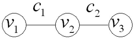
1D graph. Given a three-node, two-edge graph, the vertex and edge sets are V = {v₁,v₂,v₃} and E = {e₁₂,e₂₃}. Edge weights are symmetric and have been re-labelled, c₁ and c₂, where c₁ = w₁₂ = w₂₁ and c₂ = w₂₃ = w₃₂.

Looking at the Laplacian matrix in Eqn 7 we see that the all ones vector is an eigenvector of this system, which has eigenvalue equal to zero. This means that the matrix is singular and is due to the boundary conditions implicit in this formulation of the stiffness matrix, which is that neither of the two masses at the end of the chain in Figure 1 are fixed. Intuitively this eigenvector corresponds to rigid motion of the masses. Next we consider how the WGL can be used to divide it into sub-graphs.

Partitioning a graph using a graph-Laplacian

The eigensystem of the WGL can be used to compute the diffusion kernel (Moler and Van Loan, 2003), K₂ = exp(−Lτ), i.e. the covariance of the spatial prior over GLM parameters. However, instead of computing it for a graph of dimension ~10^5-6, we approximate it by dividing it into block-diagonal form, which can be achieved using ideas from graph partitioning. The eigensystem for each block can then be computed separately. The task is to separate a graph into two subsets, V_P and $V_P^C$ (the complement of V_P), that share a minimal number of edges, where $V=\{V_P,V_P^C\}$. We have chosen to use the isoperimetric algorithm of Grady and Schwartz, 2006, instead of spectral techniques (Shi and Malik, 2000) as it involves solving a system of equations instead of an eigenvalue problem, which can improve speed and stability. An additional benefit is that it also has the potential to be used in a Mixture of Experts (Bishop and Svensen, 2003) model, which has soft instead of hard partition boundaries (see Discussion). We provide a brief outline of the algorithm here (see Grady and Schwartz, 2006 for further details) and present a summary of the steps used in our implementation.

The isoperimetric problem is; for a fixed area, find the shape with minimal perimeter (Chung, 1997). The isoperimetric number (Mohar, 1989), h_G, is the infimum of the ratio of the area of the boundary and the volume of V_P, where the boundary, |∂V_P|, is defined as $\partial V_P=\{e_{\mathit{ij}}\mid i\in V_P,j\in V_P^C\}$. The subset, V_P, can be defined by a binary indicator vector, x

$$x_i=\{\begin{array}{cc}0\mathit{if}\hfill & v_i\in V_P\hfill \\ 1\mathit{if}\hfill & v_i\in V_P^C\hfill \end{array}\phantom{\}}$$ 8

In which case, the boundary and volume of V_P are given by |∂V_P| = x^TLx and vol_VP = x^Td. The isoperimetric number is then the minimum of their ratio

$$h_G=\underset{x}{\min }\left\{\frac{x^T\mathit{Lx}}{x^{T}d}\right\}$$ 9

This minimization can be cast as the solution of a system of linear equations by allowing x to take non-negative real values (instead of binary) and solving Eqn 9 using Lagrange multipliers (Grady and Schwartz, 2006). This results in the equation, Lx = d, which can be solved by specifying a boundary condition to remove the singularity in L. The boundary condition can be thought of, in terms of the electrical circuit analogue of a graph (Strang, 2004), as equivalent to selecting a ground node (vertex). This provides the boundary condition required to render L non-singular and thereby invertible. This additional constraint amounts to removing the row and column of the ground node from the full Laplacian matrix, L, to give the reduced Laplacian, L₀. We reduce both other quantities to get

$$L_0{x}_0=d_0$$ 10

which can be solved easily, for N_V ~ 10⁵, using standard Matlab routines or relaxation methods (Press et al., 2007) for N_V > 10⁵. In the circuit analogue, the solution, x₀, is the measurement of potential at all other nodes in the circuit. This provides a function over the graph, which monotonically increases from the ground node. The vector x₀ is converted into binary form by specifying a threshold, t, i.e., V_P = {v_i | x_i ≤ t} and $V_P^C=\{v_i\mid x_i>t\}$. This partition is referred to as a cut. Each segment can then be divided again⁵, resulting in a recursive partitioning algorithm.

The ground node can be selected in a number of ways; either the node with maximal degree or at random. We have chosen the latter in our implementation, the steps of which are provided below:

1. Define a vertex set containing the volume to be analysed

2. Compute the graph-Laplacian for the whole graph

3. Select a ground node (at random)

4. Solve Eqn 10

5. Partition the vertex set into V_P and $V_P^C$

6. Ensure that $V_P^C$ is connected (if not, return to 3)

7. Separate the Laplacian for each segment and go to 3

8. Stop if the number of vertices of a sub-graph is below a threshold

This algorithm ensures that each segment is connected and contains a similar number of voxels. We demonstrate the algorithm for volumes of time series data in the next section and provide an illustration here using a synthetic image (i.e. these data are not over time) shown in Figure 2. This shows a partition of the image using a EGL (upper row) and GGL (lower row), i.e. where dg = 0 and dg ≠ 0 respectively (see Eqn 5). The image to be partitioned is shown in the first column, which contains two regions of pixel values greater than the surround plus low amplitude Gaussian noise. The task is to partition the image predominantly along an edge of these regions. The solution of Eqn 10 is shown in the third column, where the ground node and subsets, V_P and $V_P^C$, are indicated. A partition based on this is indicated by the thick line. The central column contains a plot of edge weights that uses the 2^nd and 3^rd eigenvectors of the graph-Laplacian as coordinates (the first eigenvector is constant). Each line segment of this plot represents an edge of the graph and is a convenient way to visualize [an]-isotropy of edge weights.

Figure 2. Synthetic image.

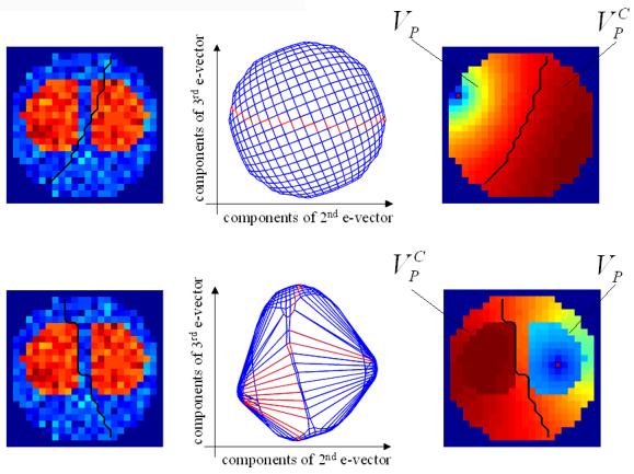
Note that there is no temporal component to these data. Partitions based on EGL and GGL are shown in the upper and lower rows respectively. Columns show (left to right) the synthetic image, to be partitioned, with a thick black line indicating the partition boundary; plot of edge weights using the 2^nd and 3^rd eigenvectors of the graph-Laplacian as coordinates to show [an]-isotropy of weights and the potential function over the graph used to determine an optimal cut. The potential function is zero at the ground node (marked pixel), which is greater than zero at all other pixels. The partition boundary is superimposed on this latter image to show that it follows a line of equal potential.

We consider first the EGL (upper row) and note that the potential function does not represent pixel values of the image. Using this function to divide the image produces a cut that passes through a region of pixels with high values, which is at odds with the task. The isotropy of edge weights (central column) can be seen as regularity in the plot, where cut edges are shown in red. As there is no preferred direction (i.e. isotropic) many different cuts can be selected given different ground nodes, the majority of which will not achieve the task. Compare this to the partition achieved using the GGL (lower row). First, we notice that the partition is predominantly along one of the steepest edges of the image. We see why this is so by examining the potential function, which now encodes pixel values as well (because dg ≠ 0). Given this function, a cut is selected, which results in a partition that respects image boundaries. The anisotropy of edge weights is seen easily in the central figure, which contains long line segments representing boundaries between high/low pixel values, i.e. ds is large (edge weight is small). In the next section, we present results applied to volumes of synthetic and real fMRI time-series data, where the spatial prior is divided into either slices or 3D segments using the WGL. We refer to a segment as being either a slice or sub-volume of a graph partition.

Results

Analysing a full volume is computationally demanding and is the reason for dividing a volume into segments. We do this in two ways; (1) dividing it into slices and (2) using the WGL to partition a volume into 3D segments. The purpose of this section is to compare the performance of models based on such divisions of a full volume. We compared them in terms of partition maps (cross-section of a volume showing partition boundaries; c.f. Figure 2), posterior mean parameter estimates, posterior probability maps (PPM)⁶ (Friston and Penny, 2003) and log-evidence. The hyperparameters of each segment were optimized using the EM scheme described in (Harrison et al., 2008).

Synthetic fMRI data

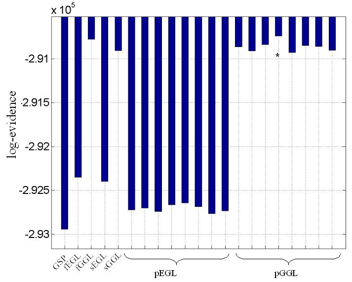
A volume of data was generated containing four slices and 1624 voxels. The main aim was to compare models using the full spatial model with those divided into segments. This led to the comparison of seven different models (1), global shrinkage prior (GSP), (2) full EGL, (3) full GGL, (4) slice-wise EGL, (5) slice-wise GGL, (6) partitioned EGL and (7) partitioned GGL. Abbreviations used for these models are given in the caption of Table 1. GSP is a spatially independent prior, i.e. K₂ = I_NV, and was included for comparison with spatial priors. As the selection of seed points (ground nodes) determines the partition in models 6 and 7, we repeated the process using eight different sets of randomly selected points. This produced eight partitions for each model.

Table 1. Log evidences for synthetic data.

Model comparison for synthetic data. Model with maximal log-evidence is shown in bold. Abbreviations; global shrinkage prior (GSP), diffusion-based spatial models applied to full volume, i.e. not divided into segments (fEGL and fGGL), applied independently to slices of a volume (sEGL and sGGL) and 3D segments using graph partitioning (pEGL and pGGL). The last two require seed points (ground nodes) to perform the segmentation, which were selected at random. This was repeated eight times to produce different partitions. The models and difference between largest (in bold) and second largest (underscored) log-evidence was for pGGL-fGGL (~40; Bayes factor > 100).

model	GSP	fEGL	fGGL	sEGL	sGGL	pEGL	pGGL
log- evidence ×105	− 2.929 4	− 2.923 5	− 2.907 8	− 2.924 0	− 2.909 1	−2.9272, − 2.9270, −2.9274, − 2.9267, −2.9264, − 2.9269, −2.9277, − 2.9273	−2.9086, − 2.9091, −2.9084, − 2.9074, −2.9093, − 2.9085, −2.9086, − 2.9090

The known parameter values of an effect of interest, design matrix and an example time-series are shown in Figure 3a. The effect of interest is encoded in the first column of the design matrix, while the remaining columns contain low-frequency oscillations to simulate scanner drift and a constant term (session mean). The known spatial pattern of response is spatially non-stationary as its smoothness varies with location. The example time series is from the marked voxel and shows the temporal profile of the effect of interest (red), scanner drift (green) and observed signal (black dashed line), which includes noise. The signal-to-noise (SNR)⁷ was approximately 1/10. Confounds were removed⁸ and data from each segment analyzed independently.

Figure 3. Synthetic fMRI data.

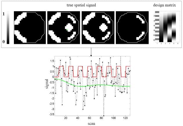
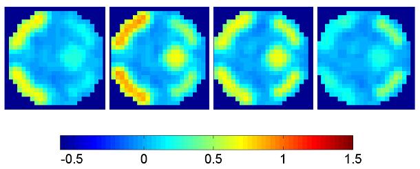
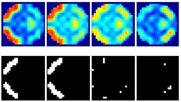
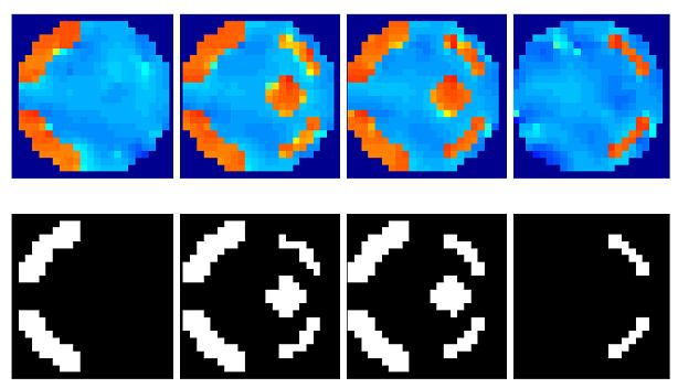
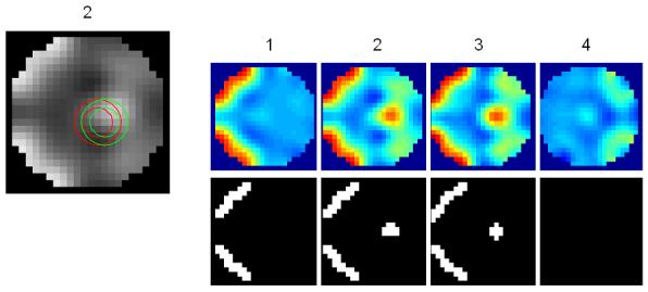
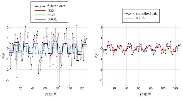
(a) A volume of data containing 1624 voxels, in 4 slices, was generated, given a known spatial response to the effect of interest. This effect is shown at the top along with the design matrix to the right. An example time series is shown from the marked voxel below, (b) OLS estimates given data smoothed by a two voxel FWHM 3D Gaussian kernel (colour scale, shown below, is common to all parameter images in Figure 3); (c-e) posterior mean estimates and PPMs (thresholds at p(u > 0.5) > 0.95) for GGL, EGL and GGL-based model using the full-graph; (f, g) same as (d, e) for volumes divided into slices with locals weights shown from the second slice on the left; (h, i) same as (f, g) for volumes divided using graph-Laplacians along with partition maps showing partition boundaries (thick white lines) overlaid on OLS estimates of non-smoothed data; and (j) Predictions from the marked voxel in a for GSP (see c) and partitioned models (see h, i) (left) and smoothed data (see b) on the right. (k) Log-evidence for all models fitted. See caption of Table 1 for abbreviations.

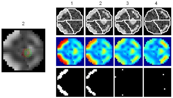
For comparison, Figure 3b shows OLS parameter estimates given data smoothed (sOLS) using a two voxel full width at half maximum (FWHM) 3D Gaussian kernel, to represent the standard mass-univariate approach used in SPM (note that the colour bar in 3b is common to all mean estimates in Figure 3). Figures 3c-e contain posterior mean estimates and PPMs using the full graph (not partitioned into segments), for GSP, EGL and GGL-based spatial models respectively. Figures 3f-g show the same for priors divided into slices, along with local weights⁹ of the diffusion kernel, while Figures 3h-i show the same for graph-partitioned priors using a EGL and GGL respectively.

First we consider the full graphs in Figures 3c-e, which illustrate the performance of GSP, EGL and GGL-based spatial models for time-series data. The posterior mean estimates of the GSP prior are noisy, suggesting the benefit of using a spatial model that includes correlations between voxels. The EGL prior is isotropic and stationary, which leads to over smoothing of boundaries between high/low regions of response. This can be seen as a blurred reconstruction of the true spatial pattern of response, which occurs within and between slices. This does not occur with the GGL-based model, which preserves functional boundaries and reduces noise within homogeneous regions. PPMs (thresholds at p(u > 0.5) > 0.95) show increased detection of the underlying signal for the GGL compared to the EGL-based model. The result is a PPM that reflects the true spatial signal more accurately than the EGL-based model.

Figures 3f-g show results where the spatial prior is divided into slices and EGL and GGL-based models applied to each independently. Local weights from the spatial covariance of parameters are shown on the left. These provide insight into the [an]-isotropy of the models, with circular kernels of the same scale at all locations in the image for EGL and kernels that adapt to functional boundaries using GGL. The issue with dividing a spatial prior into slices is that it is no longer three dimensional. As a result, edges of the original image are not all preserved (see circled regions in slices 2 and 3). An alternative that retains the priors 3D form is considered next.

Figures 3h-i show results using the graph-Laplacian to partition the prior into 3D segments. Partition boundaries are shown (thick white lines; top), which transect a region of large response (see slices 2 and 3) for the EGL. This is not so using the GGL, which partitions the parameter image along response boundaries. The effect of segmentation on local weights is to reduce their extent, however, not at the expense of adapting to functional boundaries, as seen in Figure 3i. Compared to Figure 3g, more edges of the original image are preserved. However, we now notice discontinuities in posterior estimates along partition boundaries through homogeneous regions. We address this issue in the discussion.

Predictions (along with observed time-series) from Figures 3h-i are shown in Figure 3j (left) from the marked voxel (see Figure 3a). For comparison (right), we include the prediction from smoothed data (see Figure 3b), which shows reduced amplitude of data and estimated signal. Log-evidences for all models are shown graphically in Figure 3k (see also Table 1). The greatest evidence was for a partitioned GGL-based model (pGGL). The second largest log-evidence was for the full volume (fGGL), with a difference of 40 (i.e. Bayes factor > 100). The log-evidence was greater for 7 out of 8 partitions for the GGL-based model compared to a slice-wise division of the prior. These show that partitioned GGL-based models can provide a more parsimonious model compared to priors based on the full graph and slice-wise approximation. We now compare results for real data.

High-resolution fMRI data

Here we analyse hr-fMRI data collected during a standard visual stimulation protocol used for meridian mapping. The aim was to compare spatial priors divided into slices and graph-partitions. This led to the comparison of five different models (1), global shrinkage prior (GSP), (2) slice-wise EGL, (3) slice-wise GGL, (4) partitioned EGL and (5) partitioned GGL.

These data were collected at the Wellcome Trust Centre for Neuroimaging using a 3T Siemens Allegra system with a surface coil¹⁰ centred over occipital cortex. BOLD images of retinotopic visual cortex were acquired using a multi-slice gradient echo EPI sequence, whose parameters were; 160×72 matrix, FoV = 160×72 mm², 1mm slice thickness with no gap between slices, trapezoidal EPI readout with a ramp up time of 100 ms, a flat top time of 780 ms and an echo spacing of 980 ms, slice TR 112 ms, volume TR 6720 ms, TE 45ms and 90° flip angle. Each volume contained 60 contiguous slices with 1mm² in-plane resolution and 1mm thickness. A total of 125 volumes were acquired, but the first 5 volumes were discarded prior to analysis to allow for T1-effects to stabilise.

The visual stimulus protocol presented standard flickering (at 10Hz) checkerboard wedge stimuli either on the horizontal or vertical meridian, each for a duration of 4 image volumes. Fifteen cycles of alternating horizontal-vertical meridian stimulation (duration 8 image volumes each) were acquired. Spatial pre-processing included realignment (Friston et al., 1995) and definition of the search volume used for subsequent GLM analyses, by means of a smoothed and thresholded brain mask image where scalp tissue voxels had been manually eroded. The design matrix used for GLM parameter estimation comprised one regressor encoding the difference between periods with vertical vs horizontal meridian stimulation, as well as several confound regressors (including a constant term ; see design matrix, top left of Figure 4b).

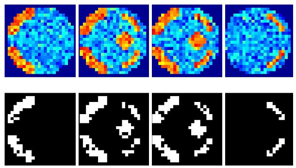
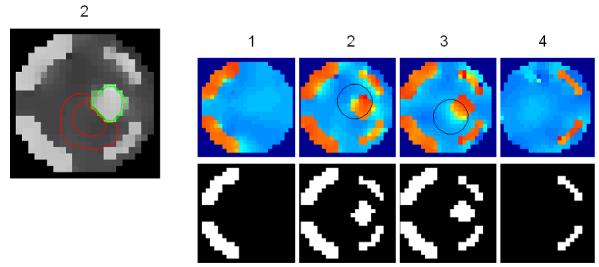
Figure 4. Real fMRI data.

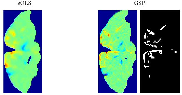
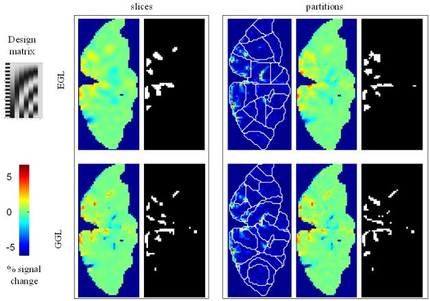
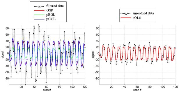
(a) OLS estimates from a transverse slice using smoothed data (left) and posterior mean estimates (see colour scale in 4b) and PPM (thresholds at p(u > 5) > 0.95) for the GSP (right). (b) design matrix and percentage signal change (colour scale common to all parameter images) shown on the left. Posterior mean estimates, PPMs for volumes divided into slices (left box) and graph partitions for EGL (top row) and GGL priors. Partition boundaries are also shown overlaid on the absolute values of OLS estimates of non-smoothed data, (c) prediction from the marked voxel for non-smoothed data, analysed using graph-partitioned priors (left) and mass-univariate approach using smoothed data (right). (d) Log-evidence for all models used. See Table 1 caption for abbreviations.

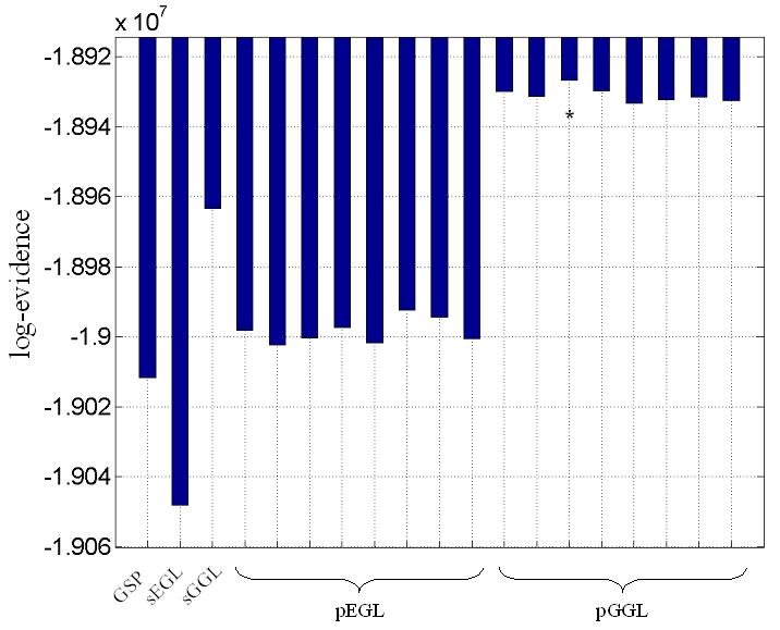
The volume analysed contained forty slices, which comprised ~75,000 voxels. The average time to process this volume was ~60 minutes using a computer with clock rate 3.06GHz and 2Gb of RAM (~0.05 seconds/voxel). The time to segment this volume was ~20 minutes. The main effect of visual stimulation (horizontal vs vertical meridian; first column of design matrix; top left) from a transverse slice is shown for data smoothed using a 2mm FWHM Gaussian (sOLS) in Figure 4a (left; see color scale in 4b). Posterior mean estimates and a PPM (right; thresholds at p(u > 5) > 0.95), which correspond to maps of voxels where the model is 95% confident that the effect size is greater than 5% of the global mean) for the spatially independent prior (GSP) show a noisy response, however, there is clear spatial structure. Posterior mean estimates (colour scale to the left indicates percent signal change), PPMs and partition boundaries are shown in Figure 4b for EGL-based (top row) and GGL-based models, where the left and right boxes contain results from volumes divided into slices and 3D segments using graph partitioning respectively. The partition boundaries from EGL and GGL show a similar pattern as with simulated data; i.e., cuts along regions containing similar responses for GGL compared to EGL-based partitions. Comparing PPMs for all 5 models, we see reduced noise (compared to the GSP) and blurred responses for both EGL-based priors. This is in contrast to the pGGL prior (lower right), which preserves the fine spatial detail of cortical responses.

Predictions from the marked voxel (shown in Figure 4a), within a region of large response, are shown for GSP, pEGL and pGGL-based models (see Table 1 for abbreviations) in the left panel of Figure 4c along with non-smoothed data from that voxel. This shows similar predicted responses for GSP and pGGL-based models, which (visually) provide a good explanation of the data. In contrast, the prediction using the EGL-based model is poor. A similar effect is seen in the right panel for data that has been smoothed with a 2mm FWHM fixed Gaussian kernel, which is common practice for hr-fMRI data (Mobbs et al., 2007; Sylvester et al., 2007). This again shows how this pre-processing step results in data that is regularized, but at the expense of its magnitude.

This is important as accurate inference over a volume, i.e. family of voxels, requires taking into consideration correlations between data points to appropriately protect again false positives. In SPM this is achieved by estimating the spatial smoothness of residuals and using results from random field theory (RFT) to correct test statistics computed at each voxel independently (Worsley et al., 1996). To ensure the assumptions of RFT are not violated, data is typically smoothed (see Chapter 2 of (Friston et al., 2006)). However, neuroimagers may not smooth data so as to preserve fine spatial detail in high resolution data. An explicit spatial model of dependence between voxels provides an alternative, where the posterior covariance encodes this dependence and can be used to make inference over a family of voxels. In particular, the GGL-based model allows for non-stationary/non-isotropic smoothness, which leads to preservation of fine spatial detail.

Discussion

The motivation for the current development was pragmatic, in that it aimed to extend the application of diffusion-based spatial priors to large numbers of voxels, using computational resources typically available to neuroimagers to analyse data in a reasonable amount of time. This is important in order to make realistic spatial models accessible to the neuroimaging community. This is particularly relevant for high-resolution fMRI data, because these present a specific challenge to neuroimaging methods; in that investigators wish to preserve fine functional detail that could otherwise be over smoothed using conventional approaches. We have compared two different ways to approximate a spatial prior here, based on dividing a volume into slices and graph partitions using a WGL, which we also compared to a model comprised of the full graph for synthetic data. These analyses show that a partitioned GGL-based model (pGGL) provides a parsimonious model, which is supported by the data. However, there are a number of issues to consider which we discuss next.

The issue of scalability is central to Bayesian spatial models. As there is only one model of the data, there is just one Laplacian, which is over all voxels in the brain. The associated spatial prior has a covariance matrix of the order 10^5-6, where in lies the problem. While multiple core machines and even small clusters are becoming increasingly accessible to neuroimagers, so too is the amount and complexity of data, e.g. high-resolution fMRI. Practically this means that more powerful machines are a partial and not complete solution. A regular graph could be used in an efficient algorithm, however, this would be limited to a diffusion kernel based on a EGL only. This is because the eigensystem of this graph Laplacian is known, i.e. eigenvectors are given by the discrete cosine set (Strang, 2007), and so does not need to be computed. However, this is very specialized in that as soon as we generalize to a WGL, where weights are no longer isotropic and stationary, the eigensystem needs to be computed. A simple strategy would be to restrict an analysis to a volume of interest, which is standard practice in neuroimaging, which could be achieved by first performing a standard SPM analysis using smoothed data, to produce masks of regional activity, followed by a spatial model using non-smoothed data from this smaller volume. Alternatively, a brain volume could be defined solely on grey matter tissue probability maps and a cortical representation achieved by projecting this volume onto a cortical mesh and performing the statistical analysis on the 2D embedded cortical surface (Kiebel et al., 2000). While useful for cortical structures, full 3D models are still required for sub-cortical structures.

The approach taken here was to use graphs with irregular boundaries, i.e. which excluded regions of no interest. A large number of voxels was analysed by reducing the WGL to block-diagonal form. This was achieved by dividing a volume into non-overlapping segments so that each block could be processed independently. This meant that the eigensystem of each block could be computed easily using standard routines in Matlab, which also lends itself to parallel processing. This was pragmatic and not aimed at segmenting a brain volume into biological causes of the data. While some promising results were obtained using the pGGL prior, there was an issue in that a visible impression of partition boundaries was noticed in the posterior means. This could be addressed by combining the division of a spatial prior into segments and parameter estimation using a hierarchical mixtures of experts (MoE) model (Bishop, 2006), where each segment of brain data is explained by an “expert”, which is a regression model for a specific region of anatomical space. Importantly, the probability of a voxel being generated from an expert is learnt. This is in contrast to the current approach that effectively considers the probability of belonging to an expert as either zero or one, which leads to ‘hard’ partition boundaries. This means that in the current implementation we have one expert for each segment, with no mixing between them. A benefit of a MoE formulation is that the posterior density over GLM parameters is a weighted sum over experts, which will reduce boundary effects. A similar approach has been taken by (Trujillo-Barreto et al., 2004) to analyse electrophysiological data, who refer to the probability of a class label as a ‘probabilistic mask’; however, these were not estimated and taken as known from an anatomical atlas. In addition, the ground node location used here could be included as a hyperparameter, which could be optimized similar to pseudo-inputs in (Snelson and Ghahramani, 2006). Lastly, a hierarchical MoE model could be used to optimize the number of segments as proposed in (Ueda and Ghahramani, 2002), which entails optimising the log-evidence with respect to the number of segments or mixtures.

An alternative to the large segments used here (~1-2×10³ voxels), would be to first reduce the dimensionality of a brain volume using anatomo-functional parcellation (Flandin et al., 2002; Thirion et al., 2006). The spatial priors described here could then be applied over parcels instead of voxels. A different strategy to segmenting a volume would be to compute the (reduced) eigensystem of the full WGL, which could be achieved using Nystrom method (Rasmussen and Williams, 2006) or multilevel eigensolvers (Arbenz et al., 2005) based on algebraic multigrid (AMG) (Stuben, 2001), which are designed for irregular graphs. Another promising multiscale approach is diffusion wavelets, which are an established method for fast implementation of general diffusive processes (Coifman and Maggioni, 2006; Maggioni and Mahadevan, 2006).

In summary, graph-partitioning can be used to realize sparse diffusion-based spatial priors over volumes of fMRI data. This approach may be of particular relevance to analysing high-resolution data, whose motivation is to investigate the “texture” of functional responses.

Table 2.

Log evidences for real data

Model comparison for real data. See Table 1 for abbreviations. The models and difference between largest (in bold) and second largest (underscored) log-evidence was for pGGL-sGGL (~3×10⁴; Bayes factor > 100).

model	GSP	sEGL	sGGL	pEGL	pGGL
log- evidence ×107	− 1.901 2	− 1.904 8	− 1.896 3	−1.8998, − 1.9002, −1.9000, − 1.8997, −1.9002, − 1.8992, −1.8994, − 1.9000	−1.8930, − 1.8931, −1.8927, − 1.8930, −1.8933, − 1.8932, −1.8931, − 1.8933

Appendix – H_f

In this paper the matrix that scales feature displacement (last line of Eq.5) is

$$\begin{array}{cc}\hfill & H_f=C_{\mathit{ols}}^{-1}\hfill \\ \hfill & C_{\mathit{ols}}=({\beta }_{\mathit{ols}}-M_{\mathit{ols}}){({\beta }_{\mathit{ols}}-M_{\mathit{ols}})}^T\hfill \\ \hfill & M_{\mathit{ols}}=\frac{1}{N_V}{\beta }_{\mathit{ols}}{1}_{N_V}{1}_{N_V}^T\hfill \end{array}$$ A.1

where β_ols is the OLS estimate of GLM parameters, given non-smoothed data and 1_NV is a column vector of ones length N_V.

Bibliography

- Arbenz P, Hetmaniuk UL, Lehoucq RB, Tuminaro RS. A comparison of eigensolvers for large-scale 3D modal analysis using AMG-preconditioned iterative methods. International Journal for Numerical Methods in Engineering. 2005;64:204–236. [Google Scholar]
- Ashburner J, Friston KJ. Unified segmentation. NeuroImage. 2005;26:839–851. doi: 10.1016/j.neuroimage.2005.02.018. [DOI] [PubMed] [Google Scholar]
- Aubert G, Kornprobst P. Mathematical Problems in Image Processing: Partial Differential Equations and the Calculus of Variations. Vol. 147. New York: Springer-Verlag; 2002. [Google Scholar]
- Bamberg P, Shlomo S. A course in mathematics for students of physics. Vol. 2. Cambridge: Cambridge University Press; 1990. [Google Scholar]
- Belkin M, Niyogi P. Laplacian eigenmaps for dimensionality reduction and data representation. Neural Computation. 2003;15:1373–1396. [Google Scholar]
- Belkin M, Niyogi P. Towards a theoretical foundation for Laplacian-based manifold methods. Learning Theory, Proceedings. 2005;3559:486–500. [Google Scholar]
- Bishop C. Pattern recognition for machine learning. New York: Springer; 2006. [Google Scholar]
- Bishop C, Svensen M. Bayesian hierarchical mixtures of experts. Paper presented at: Uncertainty in Artificial Intelligence. 2003 [Google Scholar]
- Branin J,FH. The Algebraic-Topological Basis for Network Analogies and the Vector Calculus; Paper presented at: Symposium on Generalized Networks; Polytechnic Institute of Brooklyn; 1966. [Google Scholar]
- Chung F. Spectral graph theory. Providence, Rhode Island: American mathematics society; 1997. [Google Scholar]
- Coifman RR, Maggioni M. Diffusion wavelets. Applied and Computational Harmonic Analysis. 2006;21:53–94. [Google Scholar]
- Dempster A, Laird N, Rubin D. Maximum likelihood from incomplete data via the EM algorithm. Journal of Royal Statistical Society Series B. 1977;39:1–38. [Google Scholar]
- Flandin G, Kherif F, Pennec X, Malandain G, Ayache N, Poline JB. Improved detection sensitivity in functional MRI data using a brain parcelling technique. Medical Image Computing and Computer-Assisted Intervention-MICCAI 2002. 2002;2488(Pt 1):467–474. [Google Scholar]
- Flandin G, Penny WD. Bayesian fMRI data analysis with sparse spatial basis function priors. NeuroImage. 2007;34:1108–1125. doi: 10.1016/j.neuroimage.2006.10.005. [DOI] [PubMed] [Google Scholar]
- Friston K, Ashburner J, Frith CD, Poline JB, Heather JD, Frackowiak RS. Spatial registration and normalization of images. Hum Brain Mapp. 1995;3:165–189. [Google Scholar]
- Friston K, Ashburner J, Kiebel S, Nichols T, Penny W. Statistical Parametric Mapping: The analysis of functional brain images. London: Elsevier; 2006. [Google Scholar]
- Friston KJ, Penny W. Posterior probability maps and SPMs. NeuroImage. 2003;19:1240–1249. doi: 10.1016/s1053-8119(03)00144-7. [DOI] [PubMed] [Google Scholar]
- Garey MR, Johnson DS. Computers and Intractability: A Guide to the Theory of NP-Completeness. W.H.Freeman & Co; 1979. [Google Scholar]
- Gautama T, Van Hulle MM. Optimal spatial regularisation of autocorrelation estimates in fMRI analysis. Neuroimage. 2004;23:1203–1216. doi: 10.1016/j.neuroimage.2004.07.048. [DOI] [PubMed] [Google Scholar]
- Gilbert JR, Miller GL, Teng S. Geometric mesh partitioning: Implementation and experiments. SIAM Journal of Scientific Computing. 1998;19:2091–2110. [Google Scholar]
- Gossl C, Auer DP, Fahrmeir L. Bayesian spatiotemporal inference in functional magnetic resonance imaging. Biometrics. 2001;57:554–562. doi: 10.1111/j.0006-341x.2001.00554.x. [DOI] [PubMed] [Google Scholar]
- Grady L. Random walks for image segmentation. IEEE Trans Pattern Anal Mach Intell. 2006;28:1768–1783. doi: 10.1109/TPAMI.2006.233. [DOI] [PubMed] [Google Scholar]
- Grady L, Schwartz EL. The graph analysis toolbox: Image processing on arbitrary graphs. Boston, MA: Boston University; 2003. [Google Scholar]
- Grady L, Schwartz EL. Isoperimetric graph partitioning for image segmentation. IEEE Trans Pattern Anal Mach Intell. 2006;28:469–475. doi: 10.1109/TPAMI.2006.57. [DOI] [PubMed] [Google Scholar]
- Gupta AK, Nagar DK. Matrix variate distributions. Boca Raton, Chapman & Hall/CRC; 2000. [Google Scholar]
- Harrison LM, Penny W, Daunizeau J, Friston KJ. Diffusion-based spatial priors for functional magnetic resonance images. NeuroImage. 2008 doi: 10.1016/j.neuroimage.2008.02.005. [DOI] [PMC free article] [PubMed] [Google Scholar]
- Held K, Rota Kops E, Krause BJ, Wells WM, 3rd, Kikinis R, Muller-Gartner HW. Markov random field segmentation of brain MR images. IEEE Trans Med Imaging. 1997;16:878–886. doi: 10.1109/42.650883. [DOI] [PubMed] [Google Scholar]
- Hendrickson B, Leland R. The Chaco User's Guide version 2.0. 1994 [Google Scholar]
- Karypis G, Kumar V. A fast and high quality multilevel scheme for partitioning irregular graphs. Siam Journal on Scientific Computing. 1998;20:359–392. [Google Scholar]
- Kass RE, Raftery AE. Bayes Factors. Journal of the American Statistical Association. 1995;90:773–795. [Google Scholar]
- Kiebel SJ, Goebel R, Friston KJ. Anatomically informed basis functions. NeuroImage. 2000;11:656–667. doi: 10.1006/nimg.1999.0542. [DOI] [PubMed] [Google Scholar]
- Kimmel R. Numerical geometry of images. New York: Springer; 2003. [Google Scholar]
- Liang L, Rehm K, Woods RP, Rottenberg DA. Automatic segmentation of left and right cerebral hemispheres from MRI brain volumes using the graph cuts algorithm. NeuroImage. 2007;34:1160–1170. doi: 10.1016/j.neuroimage.2006.07.046. [DOI] [PubMed] [Google Scholar]
- MacKay DJC. Information theory, inference, and learning algorithms. Cambridge: Cambridge University Press; 2003. [Google Scholar]
- Maggioni M, Mahadevan S. A Multiscale Framework For Markov Decision Processes using Diffusion Wavelets. Massachusetts: University of Massachusetts; 2006. [Google Scholar]
- Mobbs D, Petrovic P, Marchant JL, Hassabis D, Weiskopf N, Seymour B, Dolan RJ, Frith CD. When fear is near: threat imminence elicits prefrontal-periaqueductal gray shifts in humans. Science. 2007;317:1079–1083. doi: 10.1126/science.1144298. [DOI] [PMC free article] [PubMed] [Google Scholar]
- Mohar B. Isoperimetric Numbers of Graphs. Journal of Combinatorial Theory Series B. 1989;47:274–291. [Google Scholar]
- Moler C, Van Loan C. Nineteen dubious ways to compute the exponential of a matrix, twenty-five years later. Siam Review. 2003;45:3–49. [Google Scholar]
- Mumford D, Shah J. Optimal Approximations by Piecewise Smooth Functions and Associated Variational-Problems. Communications on Pure and Applied Mathematics. 1989;42:577–685. [Google Scholar]
- Osher S, Paragios N. Geometric Level Set Methods in Imaging Vision and Graphics. New York: Springer Verlag; 2003. [Google Scholar]
- Penny W, Flandin G, Trujillo-Barreto N. Bayesian comparison of spatially regularised general linear models. Hum Brain Mapp. 2007;28:275–293. doi: 10.1002/hbm.20327. [DOI] [PMC free article] [PubMed] [Google Scholar]
- Penny W, Friston K. Mixtures of general linear models for functional neuroimaging. IEEE Trans Med Imaging. 2003;22:504–514. doi: 10.1109/TMI.2003.809140. [DOI] [PubMed] [Google Scholar]
- Penny WD, Trujillo-Barreto NJ, Friston KJ. Bayesian fMRI time series analysis with spatial priors. NeuroImage. 2005;24:350–362. doi: 10.1016/j.neuroimage.2004.08.034. [DOI] [PubMed] [Google Scholar]
- Pham DL, Xu C, Prince JL. Current methods in medical image segmentation. Annu Rev Biomed Eng. 2000;2:315–337. doi: 10.1146/annurev.bioeng.2.1.315. [DOI] [PubMed] [Google Scholar]
- Press WH, Teukolsky SA, Vetterling WT, Flannery BP. Numerical Recipes. 3rd edn Cambridge, U.K: Cambridge University Press; 2007. [Google Scholar]
- Qui H, Hancock ER. Clustering and Embedding Using Commute Times. IEEE Transactions on Pattern Analysis and Machine Intelligence. 2007;29:1873–1890. doi: 10.1109/TPAMI.2007.1103. [DOI] [PubMed] [Google Scholar]
- Rasmussen C, Williams C. Gaussian processes for machine learning. Cambridge, Massachusetts: The MIT Press; 2006. [Google Scholar]
- Rosenberg S. The Laplacian on a Riemannian Manifold. Cambridge, U.K: Cambridge University Press; 1997. [Google Scholar]
- Shapiro LG, Stockman GC. Computer Vision. New Jersey: Prentice-Hall; 2001. [Google Scholar]
- Shi JB, Malik J. Normalized cuts and image segmentation. IEEE Transactions on Pattern Analysis and Machine Intelligence. 2000;22:888–905. [Google Scholar]
- Snelson E, Ghahramani Z. Paper presented at: Neural Information Processing Systems (NIPS) MIT Press; 2006. Sparse Gaussian processes using pseudo-inputs. [Google Scholar]
- Sochen N, Kimmel R, Malladi R. From high energy physics to low level vision. Scale-Space Theory in Computer Vision. 1997;1252:236–247. [Google Scholar]
- Song Z, Tustison N, Avants B, Gee JC. Integrated graph cuts for brain MRI segmentation. Med Image Comput Comput Assist Interv Int Conf Med Image Comput Comput Assist Interv. 2006;9:831–838. doi: 10.1007/11866763_102. [DOI] [PubMed] [Google Scholar]
- Strang G. Linear Algebra and Its Applications. Belmont, USA: Thomson Brookes/Cole; 2004. [Google Scholar]
- Strang G. Computational Science and Engineering. Wellesley-Cambridge Press; 2007. [Google Scholar]
- Stuben K. A review of algebraic multigrid. Journal of Computational and Applied Mathematics. 2001;128:281–309. [Google Scholar]
- Sylvester R, Josephs O, Driver J, Rees G. Visual FMRI responses in human superior colliculus show a temporal-nasal asymmetry that is absent in lateral geniculate and visual cortex. J Neurophysiol. 2007;97:1495–1502. doi: 10.1152/jn.00835.2006. [DOI] [PubMed] [Google Scholar]
- Tenenbaum JB, de Silva V, Langford JC. A global geometric framework for nonlinear dimensionality reduction. Science. 2000;290:2319. doi: 10.1126/science.290.5500.2319. [DOI] [PubMed] [Google Scholar]
- Thirion B, Flandin G, Pinel P, Roche A, Ciuciu P, Poline JB. Dealing with the shortcomings of spatial normalization: multi-subject parcellation of fMRI datasets. Hum Brain Mapp. 2006;27:678–693. doi: 10.1002/hbm.20210. [DOI] [PMC free article] [PubMed] [Google Scholar]
- Tolliver D, Miller GL, Collins RT. Corrected Laplacians: closer cuts and segmentation with shape priors. Paper presented at: Computer Vision and Pattern Recognition, 2005. 2005 [Google Scholar]
- Trujillo-Barreto NJ, Aubert-Vazquez E, Valdes-Sosa PA. Bayesian model averaging in EEG/MEG imaging. NeuroImage. 2004;21:1300–1319. doi: 10.1016/j.neuroimage.2003.11.008. [DOI] [PubMed] [Google Scholar]
- Ueda N, Ghahramani Z. Bayesian model search for mixture models based on optimizing variational bounds. Neural Networks. 2002;15:1223. doi: 10.1016/s0893-6080(02)00040-0. [DOI] [PubMed] [Google Scholar]
- Wells WM, Grimson WL, Kikinis R, Jolesz FA. Adaptive segmentation of MRI data. IEEE Trans Med Imaging. 1996;15:429–442. doi: 10.1109/42.511747. [DOI] [PubMed] [Google Scholar]
- Woolrich MW, Behrens TE. Variational Bayes inference of spatial mixture models for segmentation. IEEE Trans Med Imaging. 2006;25:1380–1391. doi: 10.1109/tmi.2006.880682. [DOI] [PubMed] [Google Scholar]
- Woolrich MW, Jenkinson M, Brady JM, Smith SM. Fully Bayesian spatiotemporal modeling of FMRI data. IEEE Trans Med Imaging. 2004;23:213–231. doi: 10.1109/TMI.2003.823065. [DOI] [PubMed] [Google Scholar]
- Worsley KJ. Spatial smoothing of autocorrelations to control the degrees of freedom in fMRI analysis. Neuroimage. 2005;26:635–641. doi: 10.1016/j.neuroimage.2005.02.007. [DOI] [PubMed] [Google Scholar]
- Worsley KJ, Marrett S, Neelin P, Vandal AC, Friston KJ, Evans AC. A unified statistical approach for determining significant voxels in images of cerebral activation. Hum Brain Mapp. 1996;4:58–73. doi: 10.1002/(SICI)1097-0193(1996)4:1<58::AID-HBM4>3.0.CO;2-O. [DOI] [PubMed] [Google Scholar]
- Zhang Y, Brady M, Smith S. Segmentation of brain MR images through a hidden Markov random field model and the expectation-maximization algorithm. IEEE Trans Med Imaging. 2001;20:45–57. doi: 10.1109/42.906424. [DOI] [PubMed] [Google Scholar]