Bayesian estimation of synaptic physiology from the spectral responses of neural masses

Abstract

We describe a Bayesian inference scheme for quantifying the active physiology of neuronal ensembles using local field recordings of synaptic potentials. This entails the inversion of a generative neural mass model of steady-state spectral activity. The inversion uses Expectation Maximization (EM) to furnish the posterior probability of key synaptic parameters and the marginal likelihood of the model itself. The neural mass model embeds prior knowledge pertaining to both the anatomical [synaptic] circuitry and plausible trajectories of neuronal dynamics. This model comprises a population of excitatory pyramidal cells, under local interneuron inhibition and driving excitation from layer IV stellate cells. Under quasi-stationary assumptions, the model can predict the spectral profile of local field potentials (LFP). This means model parameters can be optimised given real electrophysiological observations. The validity of inferences about synaptic parameters is demonstrated using simulated data and experimental recordings from the medial prefrontal cortex of control and isolation-reared Wistar rats. Specifically, we examined the maximum a posteriori estimates of parameters describing synaptic function in the two groups and tested predictions derived from concomitant microdialysis measures. The modelling of the LFP recordings revealed (i) a sensitization of post-synaptic excitatory responses, particularly marked in pyramidal cells, in the medial prefrontal cortex of socially isolated rats and (ii) increased neuronal adaptation. These inferences were consistent with predictions derived from experimental microdialysis measures of extracellular glutamate levels.

Introduction

The goal of neural mass modelling is to understand the neuronal architectures that might generate electrophysiological data. Key model parameters are sought, which explain observed changes in, for example, EEG spectra, particularly under pathological conditions (e.g., Liley and Bojak. 2005; Rowe et al., 2005). The ability to infer quantitative measures of microscopic synaptic function at molecular and ultra-structural levels using macroscopic electrophysiological measurements is important; it permits the use of electrophysiological data to answer questions about pathophysiological changes that are framed in terms of physiological and synaptic mechanisms. The inversion of neurobiologically grounded generative models can, in principle, quantify microscopic dynamics given macroscopic observation and thereby link the two scales.

The aim of this paper is to show how one can make inferences about synaptic function at the neuronal level using macroscopic electrophysiological measurements. In particular, we will focus on responses measured in the spectral (frequency) domain. Electrophysiologists use spectral measures of local field potentials and scalp potential recordings to investigate steady-state cortical dynamics that operate over long time periods and are not phase-locked to experimental events (David et al., 2003; Hald et al., 2006; Dumont et al,, 1999). Indeed, some brain systems have been associated with characteristic spectral behaviour; for example, the theta rhythm (4-8Hz) appears to index key operations in the hippocampus during memory consolidation (Hasselmo et al., 2002; Buzsaki, 2002; Vinogravdova, 1995).

In animal studies, microscopic physiological investigations such as microdialysis, single-cell or patch-clamp recordings are often used in conjunction with macroscopic electrophysiological measurements of population activity (Fellous et al., 2000). In humans, this is usually not feasible since, with rare exceptions (e.g., pre-surgical evaluation in epilepsy patients), experimental measurements must be non-invasive. A long-term goal of the work presented here is to enable inference about low-level physiological processes using non-invasive recordings from the human brain (Stephan et al., 2006), within a model-based approach. This paper is a step towards this goal, in which we demonstrate the plausibility of the approach using invasive animal data.

There are several features of the EEG that demonstrate clear differences between normal and pathologic conditions (Hughes and John, 1999). Examples include differences in the P300 component of event-related potentials between Alzheimer’s patients and controls (Polich, and Pitzer, 1999); differences in background spectral band power reported for several neurological and neuropsychiatric diseases (e.g., Fenton et al., 1980; Tanaka et al., 2000) and differences in chaotic dimensions from single-trial time series (Hornero et al., 1999) in schizophrenia. A key distinction between these approaches, and the one adopted here, is that previous approaches are descriptive, aiming to find discriminative features of the data. In contrast, our approach is mechanistic and tries to characterise pathophysiological processes through inference on the parameters of a biophysical model. These parameters may encode fundamental synaptic physiological differences between normal and diseased subjects. The model we consider here comprises interacting neural masses, which constitute cortical or subcortical sources of electromagnetic activity. Our approach accommodates neurobiologically plausible interactions within and among sources. For simplicity, in this paper, we focus on a single source model.

In previous work (Moran et al., 2007), we proposed a generative or forward model of spectral output based on an established neural mass model of cortical dynamics (Jansen and Rit, 1995). This was an extension of a model that has been characterised extensively in the literature (e.g., David et al, 2005 and references therein). The extensions included recurrent inhibitory connections and an explicit parameterization of neuronal adaptation. The model’s dynamics were examined in a linear setting to establish the values of various parameters leading to stable steady-state dynamics. The linearity assumption is used widely in the context of spectral analysis; for example, estimation of frequency spectra pervades the literature regarding cortical rhythms. The linear framework treats the neural mass as a system that is perturbed by white noise; analogous to non-specific afferents. This provides a compact summary of the system in terms of its transfer function, H(s), where the output (under flat spectral input) can be obtained from the magnitude of H(s) directly. The transfer function depends on the physiological parameters of the model. Therefore, the transfer function links unobserved physiological processes to measured spectral responses and is an essential part of the forward or generative model of spectral measures.

Bayesian inversion of this model provides the posterior probability densities of the model parameters. The variational expectation maximisation (EM) scheme employed below has been applied successfully to similar input-state-output systems to produce Dynamic Causal Models (DCMs) of event-related potentials (ERPs). These models allow for inference on the deployment of sources and the connections among sources during stimulation (David et al., 2006, Kiebel et al., 2006). This paper describes a DCM for the spectral domain that can be used to model steady-state or induced responses.

The paper comprises two sections. The first section describes the equations controlling the evolution of the local field potential of a neural mass. The transfer function associated with these equations is used as the basis of a likelihood model for observed spectral activity. The prior density assumptions are then described. Together, the likelihood and prior densities constitute a generative model, which can be inverted given some data. Finally, we consider the inversion scheme for deriving the posterior or conditional estimates of the model parameters. The second section tries to establish the models face and construct validity using simulated and empirical data. We analyse efficiency and robustness, using synthetic data generated with different noise levels and parameter values, respectively. The final analysis addresses construct-validity using empirical LFP data. This necessitated the use of an animal model where other invasive measurements were available to corroborate the analysis of the LFP. Specifically, we studied a rodent model of schizophrenia, the isolation-rearing model (Geyer et al., 2001). Radio-telemetric data (EEG), via a subdural electrode (Siedenbecher et al., 2003), and extracellular glutamate and γ -aminobutyric acid (GABA) levels, via microdialysis probe (Brady et al., 2005; De Souza et al., 2005), were obtained from the medial prefrontal cortex of social and isolated rats. This allowed us to compare conditional estimates of synaptic function with predictions derived from the empirical measures of extracellular glutamate and GABA levels.

A neural mass model of spectral activity

Spectral Responses of a Neural Mass Model

In a spectral formulation of neural mass models, we assume that the source of LFP or EEG applies a filter-like operation to its inputs so that the input frequencies are modulated by its transfer function, H(s), where s denotes a location in the complex s-plane encoding damped oscillatory dynamics. In linear systems analysis, the Laplace transform allows one to formulate the system’s time-domain equations of motion in terms of frequency domain operators that are characterized by the system’s transfer function (see Figure 1). This allows us to express the output Y(s), in response to an input, U(s) in the frequency domain, directly.

$$Y\left(s\right)=H\left(s\right)U\left(s\right)$$ (1)

Fig. 1.

Conversion scheme to obtain spectral outputs from the systems transfer function

We model a single source as a microcircuit, in which three neuronal populations are assigned to three cortical layers (infragranular, granular and supragranular; see Fig. 2). Different sources can be connected through forward, backward and lateral connections, with laminar-specific patterns of origin and termination that conform to neuroanatomical studies (Felleman and Van Essen 1991); however, here we consider just one source. Within each source, a population of excitatory pyramidal (output) cells receives inputs from inhibitory and excitatory populations of interneurons via intrinsic connections. In this model, excitatory interneurons are spiny stellate (input) cells, which are found in layer IV and receive forward connections (or subcortical inputs). Although pyramidal cells and inhibitory interneurons are found in both infra- and supragranular layers in cortex, we assign each population to a single layer for simplicity (David et al. (2006). The three neuronal populations are connected as shown in Fig. 2, with intrinsic coupling parameters, γ_i. Neuronal populations are modelled with linearly separable synaptic responses to excitatory and inhibitory inputs. Importantly, the (dendritic) membrane potential of pyramidal cells provides the cortical output as measured with the LFP or EEG. This is based on the fact that the apical dendrites of these cells orient perpendicularly to the cortical surface, providing congruent post-synaptic potentials.

Fig. 2.

Equations of motion for a single source comprising three neural masses or populations. The insets show the impulse response kernel and firing rate-input curves

There are two key operators that describe the behaviour of the neuronal populations. The first transforms u(t), the average density of pre-synaptic input arriving at the population, into v(t), the average postsynaptic membrane potential (PSP). This can be modelled by convolving the input with a parameterised impulse response function h_e/i(t). The synapse operates as either inhibitory or excitatory, (e/i), such that

$$\begin{array}{c}\hfill v\left(t\right)=h_{e∕i}\left(t\right)\otimes u\left(t\right)\hfill \\ \hfill h_{e∕i}\left(t\right)=H_{e∕i}{\kappa }_{e∕i}t\exp (-t{\kappa }_{e∕i})\hfill \end{array}$$ (2)

The parameter H tunes the maximum amplitude of PSPs, and κ = 1/τ is a lumped representation of the rate constants (inverse time-constants) of passive membrane and other spatially distributed delays in the dendritic tree. This synaptic convolution can be formulated in terms of a kernel or a state-space representation using equations of motion $\stackrel{.}{x}=f\left(x\right)$, where $x\in \{v,\stackrel{.}{v}\}$ (see Fig. 2 and David et al., 2003).

The second operator transforms the average membrane potential of the population into the average rate of action potentials fired by the neurons. This transformation is assumed to be instantaneous and is described by the sigmoid function

$$S\left(v\right)=\frac{1}{1+\exp (-{\rho }_1(v-{\rho }_2))}-\frac{1}{1+\exp \left({\rho }_1{\rho }_2\right)}$$ (3)

where ρ₁ and ρ₂ are parameters that determine its shape (c.f., voltage sensitivity) and position respectively. It is this function that endows the model with nonlinear behaviour and biological plausibility. Its motivation comes from the fact that firing thresholds vary over a population or ensemble of many neurons (Freeman 1972). The parameter ρ₂ can be regarded as modelling adaptation currents, such that increases in adaptation reduce the sensitivity or gain of the relationship between the average membrane potential and firing rate (see Fig. 3). This models steady-state changes in synaptic firing induced by neuromodulatory effects (e.g., pharmacological manipulations). In brief, ρ₂ is a lumped representation of the effect of several currents, including voltage-gated potassium currents, calcium-gated potassium channels and the slow recovery from inactivation of the fast sodium current; these currents tend to shift the firing rate-input to the right (see Benda and Herz, 2003), causing the firing rate to drop for a given membrane potential.

Fig. 3.

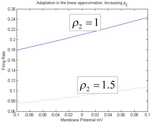
Increasing the adaptation parameter produces a decreased neural output firing rate and sensitivity (i.e., gain) for any given membrane potential. The linear approximation holds for small perturbations around a stead-state equilibrium membrane potential.

Finally, a parameter, d controls intrinsic conduction delays between populations of neurons. In summary, the neurophysiology of the source or neural mass is determined by the twelve parameters, θ ⊆ ρ₁,ρ₂,τ_e,τ_i,H_e,H_i,γ₁,γ₂,γ₃,γ₄,γ₅,d, representing sigmoid parameters, synaptic parameters, intrinsic connection strengths, and conduction delay.

The likelihood model

To estimate these physiological parameters, we need to specify a generative model that comprises a likelihood function and priors on the parameters. The likelihood function enables us to specify the probability of any output given some model parameters and input. This probability is defined by assuming the difference between what is observed and what is predicted is well-behaved observation noise. In this case, the observed output is the energy spectrum or power across the frequencies encountered in the EEG and LFP, encompassing 0⁺- 60 Hz, (i.e., delta (0-4), theta (4-8), alpha (8-16), beta (16-30) and gamma (30-60) bands). The predicted output is determined by the transfer function, under simplifying assumptions about the spectral properties of the input. Transfer functions are properties of linear systems and so we approximate the sigmoid function with a linear Taylor expansion S(v) = [∂S/∂v]v around the equilibrium point v = 0. This assumes small perturbations of neuronal states around steady-state, where

$${\phantom{\mid }\frac{\partial S}{\partial v}=\frac{{\rho }_1\exp \left({\rho }_1{\rho }_2\right)}{{(1+\exp \left({\rho }_1{\rho }_2\right))}^2}\mid }_{v=0}$$ (4)

After linearization changes in gain ∂S/∂v produced by changes in ρ₁ and ρ₂ have a very similar effect. We can accommodate this by keeping ρ₁ fixed and restricting our inference to ρ₂. Linearising the model in this way allows us to evaluate the transfer function

$$H\left(s\right)=C{(sI-A)}^{-1}B$$ (5)

where, A = ∂f/∂x, B = ∂f/∂u and C is a row vector that constrains the measured output to the pyramidal cell depolarisation, x₉. These matrices depend on the parameters which parameterise the equations of motion f(x,θ); see Fig. 2.

The frequency response for steady-state input oscillations at ω radians per second obtains by evaluating Eq.5 at s = jω (where jω represents the axis of the complex s-plane corresponding to steady-state frequency responses). In the case of unknown afferent input, we assume white noise (Wright et al., 1994). This corresponds to a flat spectral input and is the standard for system characterization (Chichilnisky, 2001). The output frequency spectrum is now simply the magnitude of the system’s transfer function.

$$\mid Y\left(j\omega \right)\mid =\mid H\left(j\omega \right)\mid$$ (6)

When the system is driven by a stimulus with a known spectrum, U (jω), the output becomes the frequency profile of the stimulus modulated by the transfer function

$$\mid Y\left(j\omega \right)\mid =\mid H\left(j\omega \right)\mid \mid U\left(j\omega \right)\mid$$ (7)

Real LFP and EEG recordings contain non-specific components from nearby sources. We model these as a mixture of white and pink, or 1/f, noise, where f = 2πω. Pink noise exhibits the ubiquitous 1/f spectrum seen in steady-state EEG spectral measures. This spectral component has been shown to be insensitive to pre- and post-sensory excitation differences (Barrie et al., 1996), and may represent non-specific desynchronisation (Lopes da Silva, 1991; Accardo et al, 1997). Its form, where the log of spectral magnitude decreases linearly with the log of the frequency, is thought to arise as a general property of closed medium wave propagation (Barlow, 1993; Jirsa and Haken 1996; Robinson 2005). In light of this, we assume the observed spectrum is a mixture of a spatially distributed 1/f component and a regionally specific component modelled with our neural masses. The resulting full observation model for measured log-spectral output at frequency ω_i is then

$$\begin{array}{c}G\left({\omega }_i\right)=\zeta \left({\omega }_i\right)+{\epsilon }_i\hfill \\ \zeta \left({\omega }_i\right)=\ln ({\beta }_1{\mid Y\left(j{\omega }_i\right)\mid }^2+{\beta }_2+{\beta }_3∕{\omega }_i)\hfill \end{array}$$ (8)

where β ∈ {β₁,β₂,β₃} controls the relative power of the modelled source, white and pink physiological noise respectively. For clarity, we will absorb these coefficients into the vector of free parameters; θ → {θ,β }. Notice that we have log-transformed the predicted power. This ensures our assumptions about observation noise are more tenable¹. Observation noise, ε (which is distinct from the random physiological fluctuations) is assumed to be Gaussian with zero mean and unknown covariance, λQ. λ is a variance hyperparameter controlling the amount of noise whose correlations are encoded by Q. Under this assumption, the likelihood is simply

$$p(G\mid \theta ,\lambda )=N(\zeta \left(\theta \right),\lambda Q)$$ (9)

The posterior probability p(θ | G,λ) of these parameters is proportional to the likelihood of obtaining the measured power spectrum p(G | θ,λ) times the prior probability, p(θ); these priors are required to complete our specification of the generative model.

The priors

We assume that priors conform to Gaussian probability density distributions. This means that prior densities can be specified in terms of their expectation and covariance. The expectations of these parameters are biologically plausible amplitudes and rate constants that have been used in previous instances of the model (Jansen et al., 1992; David et al., 2005). The original motivation for these values is described in Jansen and Rit (1995), and is based mainly on animal studies. The prior expectations used in this work are shown in Table 1.

Table 1.

[Log-normal] priors on physiological parameters

Parameter θi = μi exp(i)	Physiological Interpretation	Prior:
		Mean: μi	Variance: i ~ N(0, C)
ρ1,ρ2	Parameters of firing-rate-input function (amplitude and adaptation)	μρ1 = 2 μρ2 = 1	C = 1/8 C = 1/8
τe/i = 1/κe/i	Average synaptic time-constant	μτe = 4msec μτi = 16msec	C = 1/8 C = 1/8
He/i	Maximum post-synaptic potential (amplitude of synaptic kernel)	μHe = 4mV μHi = 16mV	C = 1/8 C = 1/8
γ 1,2,3,4,5	Efficacy of synaptic connections among populations	μγ1 = 128 μγ2 = 128 μγ3 = 64 μγ4 = 64 μγ5 = 16	C = 1/8 C = 1/8 C = 1/8 C = 1/8 C = 1/8
d	Intrinsic conduction delay	μd = 2m sec	C = 1/2

The dynamics associated with different parameter values can also inform our choice of priors: Transfer functions are known as BIBO stable, when a bounded input (BI) yields a bounded output (BO). This is an intuitive and necessary condition for healthy cortical dynamics. The parameter values that conform to these BIBO conditions were established in Moran et al. (2007). Briefly, for stability, necessary and sufficient conditions arise when the roots of the denominator of the transfer function (known as the system poles) remain inside the unit circle in the z-plane (the discrete analogue to the Laplacian s-domain). Parameters were scaled from one quarter to four times their prior expectation and stable BIBO dynamics were established for this range. Figure 4 presents an example of this analysis, where the system poles are tracked for the excitatory time constantτ_e (see Moran et al., 2007 for more details).

Fig. 4.

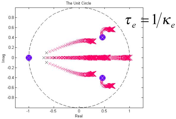
Stability analysis for the excitatory time-constant; which was scaled from one quarter to four times its prior expectation of 4mV. Stability is characterised by the movement of the poles with changes in a parameter (red crosses). If the poles remain within the unit circle the system is stable. The complete system representation also includes the system zeros (area of zero frequency output); these are the roots of the transfer functions numerator and are depicted as blue circles. The crosses and circles increase in size with increasing time-constants (from 1 to 16mV). The real positive half of the unit circle axis encompasses frequencies from 0 to 60Hz. The system response at these frequencies can be regarded as the distance from the axial frequency point to each zero (the product of all distances), divided by the distance from that frequency to the poles (hence poles on the unit circle present an infinite unbounded output, and a zero on the unit circle represents zero frequency response).

In our model, all the parameters θ are positive variables and rate-constants and so we re-parameterise with θ_i = μ_i exp(_i), where μ_i is the prior mode and exp(_i) is a scale parameter. This formulation rests on a zero mean Gaussian prior p(_i) = N(0,C) for _i. This implicitly provides a log-normal prior density on the parameters (see Table 1), where, effectively, the prior mean enters as a fixed parameter of the model. A variance of C ≈ 1/2 corresponds to a rather uninformative prior that allows θ_i to vary by an order of magnitude. Conversely, C ≈ 1/8 corresponds to an informative prior and will only allow variations of about fifty percent around the prior expectation. We used C ≈ 1/8, which ensures stability (see Table 1 and Fig. 4) and reflects our formal knowledge of the underlying dynamics. Equipped with these priors, a full Bayesian estimation of the particular parameters producing the data can proceed.

Bayesian inversion

In Bayesian inference, prior beliefs about model parameters are quantified by the prior, p(θ). Inference on θ after observing data, G rests on the posterior density p(θ | G). These densities are related using Bayes rule

$$p(\theta \mid G)\propto p(G\mid \theta )p\left(\theta \right)$$ (10)

where p(G | θ) is the likelihood. The posterior density is an optimal combination of prior knowledge and new observations, weighted by their relative precision (i.e., inverse variance); it provides a complete description of uncertainty about the parameters, given prior knowledge. The Maximum a Posteriori or MAP estimate is simply

$${\theta }_{\text{MAP}}=\underset{\theta }{\max }p(\theta \mid G)$$ (11)

Special cases of this estimate are used in classical estimation schemes. For example, when the priors are flat (i.e., a uninformative or uniform prior) one obtains

$${\theta }_{\text{MAP}}={\theta }_{MI}=\underset{\theta }{\mathit{max}}p(G\mid \theta )$$ (12)

where, θ_ML is the Maximum Likelihood estimate, which does not include prior information about the parameters. Priors are included in Bayesian schemes to place constraints on model parameters. Using human and animal data, Jansen and Rit (1993; 1995) outlined synaptic parameter values that are biologically plausible and generate typical EEG spectra and ERPs. This information is embodied in the priors used here. Generally, the choice of priors can either reflect empirical knowledge (e.g., previous measurements) or formal considerations (e.g., some parameters cannot have negative values).

In variational approaches to inverting generative models, the moments of the posterior density (conditional mean η and covariance Σ) are updated iteratively under a fixed-form Laplace (i.e., Gaussian) approximation to the conditional density, q(θ) = N(ν,Σ). If we assume the variance hyperparameter has a point mass, then these updates can be regarded as an Expectation-Maximization (EM) scheme. The E-step performs an ascent on a variational bound to optimise the conditional moments. In the M-Step, the variance hyperparameters λ are updated in exactly the same way. The variational bound that is maximised is the free energy:

$$\begin{array}{c}F=\ln p(G\mid \lambda )-KL[q\left(\theta \right),p(\theta \mid G,\lambda )]\hfill \\ \mathbf{E}-\text{step}\eta =\underset{\eta }{\mathit{max}}F\hfill \\ \mathbf{M}-\text{step}\lambda =\underset{\lambda }{\max }F\hfill \end{array}$$ (13)

When the free energy is maximised the Kullback-Leibler (KL) divergence term becomes small and q(θ) ≈ p(θ | G,λ). Note that the conditional covariance is not optimised explicitly because, under the Laplace assumption, it is an analytic function of the conditional mean. For dynamic models of the sort presented in this paper, this approach has been evaluated in relation to Monte Carlo Markov chain (MCMC) techniques and has been found to be robust, providing accurate posterior estimates while being far superior in terms of computational efficiency (see Friston et al. 2006). It is important to note that the use of priors cannot bias one towards false inference; this is because tighter priors shrink estimates to their prior means and suppress differences in their conditional estimate.

Following Friston et al. (2002; 2006) our E-step employs a local linear approximation of Eq. (8) about the current conditional expectation

$$\begin{array}{c}\hfill G-\zeta \left(\eta \right)\approx J\Delta \vartheta +\epsilon \hfill \\ \hfill \Delta \vartheta =\vartheta -\eta \hfill \\ \hfill J=\frac{\partial \zeta \left(\eta \right)}{\partial \vartheta }\hfill \end{array}$$ (14)

This local linear approximation allows one to perform a gradient ascent on the free energy to optimise the posterior moments. The M-step performs an ascent on the free energy to update the hyperparameter, λ. This is repeated until convergence

$$\begin{array}{c}\mathbf{E}-\text{step}\hfill \\ \stackrel{‒}{G}=\left[\begin{array}{c}\hfill G-\zeta \left(\eta \right)\hfill \\ \hfill -\eta \hfill \end{array}\right]\stackrel{‒}{J}=\left[\begin{array}{c}\hfill J\hfill \\ \hfill I\hfill \end{array}\right]\stackrel{‒}{C}=\left[\begin{array}{cc}\hfill \lambda Q\hfill & \hfill 0\hfill \\ \hfill 0\hfill & \hfill C_{\vartheta }\hfill \end{array}\right]\hfill \\ \Sigma ={\left({\stackrel{‒}{J}}^T{\stackrel{‒}{C}}^{-1}\stackrel{‒}{J}\right)}^{-1}\hfill \\ \Delta \eta =\Sigma \left({\stackrel{‒}{J}}^T{\stackrel{‒}{C}}^{-1}\stackrel{‒}{G}\right)\hfill \\ \mathbf{M}-\text{step}\hfill \\ P={\stackrel{‒}{C}}^{-1}-{\stackrel{‒}{C}}^{-1}\stackrel{‒}{J}\Sigma {\stackrel{‒}{J}}^T{\stackrel{‒}{C}}^{-1}\hfill \\ F_{\lambda }=-\frac{1}{2}tr\left(PQ\right)+\frac{1}{2}{\stackrel{‒}{G}}^T{P}^{T}QP\stackrel{‒}{G}\hfill \\ F_{\lambda \lambda }=-\frac{1}{2}tr\left(PQPQ\right)\hfill \\ \Delta \lambda =-F_{\lambda \lambda }^{-1}{F}_{\lambda }\hfill \end{array}$$ (15)

We use Q = I, assuming measurement error that is independently and identically distributed across frequencies (in log-space).

The scheme affords an efficient way to obtain the posterior density of the parameters of our model. Although we will focus on the conditional means, the conditional covariances also contain important information about dependencies among parameter estimates. These can arise when changes in different parameters are expressed in a similar way in the data. Fig.6 shows an example using empirical data (from a control rat analysed in the final section). Here, we have normalised the posterior covariance matrix to produce a correlation matrix. Fig.6 shows that most of the parameters have very small correlations; however, ρ₁ and ρ₂ are negatively correlated (suggesting they have positively correlated effects in data space). This means that if one is interested in one of the sigmoid parameters, the other can be fixed to suppress redundancy. In the next section, we apply the theory above to synthetic and real data to see if we can recover meaningful model parameters from observed data.

Fig. 6.

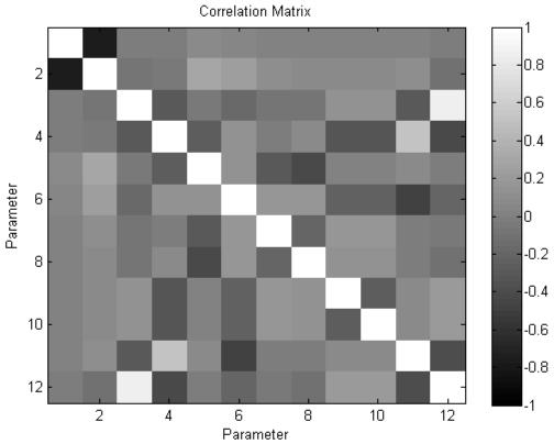
Conditional dependencies between ρ₁ and ρ₂ are revealed in terms of a posterior covariance matrix (normalised to a correlation matrix for visual inspection). The high values of Σ₁₂ and Σ₂₁ reveal correlations between the sigmoid parameters. Other parameters do not exhibit high interdependence and are estimated efficiently (i.e., with high precision).

Model validation

Simulations

In this section, we demonstrate the methodology using synthetic and empirical data. In our simulations, data were generated using Eq.5, with frequencies from 0⁺ to 50 Hz. Two important aspects of the inversion were addressed. In the first set of simulations we examined the sensitivity or efficiency of the scheme. This involved assessing the precision with which various parameters could be estimated under different levels of measurement noise. The second set of simulations looked at posterior means, when the true parameter values deviate from their prior expectation. This assesses how the inversion behaves when the system operates in regions of parameter space that are remote from the prior assumptions.

Efficiency under different levels of noise

In these analyses, data were simulated with various levels of noise. We generated frequency responses using the prior expectation of the parameters and then added noise after log-transforming. The levels of noise were based on the variance hyperparameter estimates of the empirical dataset (a social baseline animal; see below). The noise was then scaled from exp(-4) to exp(6) times this empirical level. Figure 7 shows representative parameter estimates, in terms of their 90% confidence intervals (Bayesian credible intervals) as a function of noise variance. Dashed lines show the true parameter values. These results are representative of the whole set of simulations and reflect accurate parameter estimates across large ranges of noise. Note that the conditional uncertainty is bounded by the prior uncertainty; this can be seen by increasing confidence intervals that asymptote to the prior confidence intervals at very high noise levels (this effect is most obvious for parameter H_e, in Figure 7a). Figure 7d shows the asymptotic behaviour of the posterior variance estimate of parameter, γ₅, this parameter was given a prior variance of 1/8 and approaches this value in high noise levels. Overall, the conditional means remained close to the true values for all parameters, despite differences in their conditional precision.

Fig. 7.

Results of parameter estimation using synthetic data in the presence of noise; parameter estimates, plotted with 90% confidence intervals in grey. The x-axis is the scaled noise variance. Dashed red lines show the true parameter value. A) Maximum Excitatory Postsynaptic Potential, H_e B) Pyramidal Cell to Stellate Connectivity, γ₂ C) Recurrent Inhibitory Connectivity, γ₅ D) Posterior variance estimate for parameterγ₅, in increasing levels of noise.

Accuracy under different parameter values

We next investigated the behaviour of the conditional estimates when true parameter values deviate markedly from their prior expectation. Spectral responses were synthesised using parameter values equal to the prior expectation, with the exception of the parameter under test; which was scaled from exp(-0.5) to exp(0.5) of its prior mean. This addresses the applicability of our model to neural masses with ‘unusual’ parameters. Two exemplar parameters were examined, namely, the adaptation parameter ρ₂ and the inhibitory post-synaptic time-constant, τ_i = 1/κ_i .

The conditional estimates and their true values are presented in Fig. 8, along with the spectral fits obtained for synthesized data (at a scaling by exp(0.5) of the prior mean). These results show that the true value can be estimated when our prior assumptions are not veridical. Note the characteristic regression or ‘shrinkage’ of the posterior mean to the prior mean in the case of very low ρ₂. This reflects the use of shrinkage priors in the Bayesian inversion scheme. The inhibitory time constant τ_i however, is estimated well for all simulated changes. In summary, the scheme seems to afford accurate predictions over a reasonable domain of parameter space.

Fig. 8.

Results of the second simulations, showing estimated (dark line) and true (dashed line) parameter values for the adaptation parameter (left) and the inhibitory time constant (right). 90% confidence intervals are shown in grey. The bottom panel shows the spectral fits for models where parameters are simulated at exp(0.5) times their prior expectation (true spectra; dashed red line, model fit; dark line)

Empirical LFP studies

The final validation comprised an inversion of the model using empirical LFP recordings from embedded electrodes in the prefrontal cortex of normal rats and isolation reared counterparts. These data came from a study of a rat model of schizophrenia, the isolation-rearing model (Geyer et al., 2001). In this model, Wistar rats are taken at weaning (postnatal day 25) and housed alone; devoid of contact with other animals or environmental stimulation. When compared to socially-housed control counterparts, isolated rats exhibit deficits akin to those seen in schizophrenic patients, as measured by a putative schizophrenia endophenotype, i.e., pre-pulse inhibition of startle (Geyer et al., 1993).

For the present analysis, local field potential (LFP) data were recorded by means of a deep-implanted electrode (Siedenbecher et al., 2003) and a radio-telemetric system (Data Sciences International, St Paul, MN, USA). LFPs were recorded over a 24h period from the prefrontal cortex of six isolated and six socially raised animals. During the recordings, the animals were moving freely in their home cage and not exposed to external stimuli. The data analysed here were spectral responses averaged over epochs covering a ten-minute period. The neural mass model of the previous section was fitted separately to the data from each rat. To establish construct validity, we compared the ensuing parameter estimates with predictions that were derived from microdialysis measurements of extracellular glutamate and γ -aminobutyric acid (GABA) levels in a separate group of six social and six isolated rats. Note that electrophysiological recordings and microdialysis measures were obtained from separate animals; therefore, our comparisons are not performed within individual animals, but at the group level.

It should be noted that changes in extracellular transmitter levels and estimates of synaptic parameters in our model do not have a direct one-to-one relationship. Chronic alterations of extracellular transmitter levels, induced by social manipulations can be produced by different neurobiological mechanisms; i.e., changes in neurotransmission itself, changes in transmitter metabolism by glial cells or changes in transmitter reuptake. For example, disruption of glutamate reuptake by reduced transporter activity results in accumulation of neurotransmitters (Jabaudon et al., 1999; Gegelashvili et al., 1997; Ishiwari et al., 2004). However, whatever the cause of transmitter level changes, we can make precise predictions about the consequences of these changes on synaptic transmission and therefore about the expected changes in our model parameters. For example, a chronic increase in extracellular glutamate levels leads to down-regulation of associated post-synaptic receptors and a reduction in excitatory post-synaptic potentials, i.e., de-sensitization of excitatory post-synaptic responses (Oliet et al., 2001). Conversely, a lasting decrease of extracellular glutamate induces up-regulation and sensitisation of postsynaptic glutamate receptors (Van den Pol et al. 1996).

Figure 9 illustrates the mean power spectra in each group. A descriptive analysis demonstrates that the two groups exhibit significant differences in recorded LFP spectra: a two-sample t-test, applied to each 5Hz frequency bin, showed significant between-group differences (p<0.05 corrected for multiple comparisons) for frequencies below 10 Hz and in the high-alpha/low-beta band at 15-10Hz (see astrix: Fig. 9). These differences in the measured spectra suggest that one should see significant differences in our parameter estimates, when fitting the model to data from both groups. To establish construct validity we used the empirical microdialysis measures to predict which parameter estimates should differ most and in which direction:

Fig. 9.

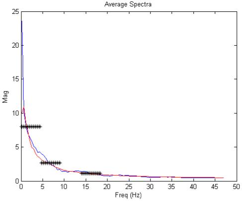
Average Spectra of isolated (red) and control (blue) animals. Significant between-group differences (p<0.05 corrected for multiple comparisons and binned to mean freq across 5Hz) are indicated by an astrix.

The microdialysis measures showed a profound reduction in extracellular glutamate levels in the prefrontal region of the isolated rats² (Table 2; Brady et al., 2005; De Souza et al., 2005). Reduction in extracellular glutamate levels is associated with a sensitization of post-synaptic mechanisms, e.g. by means of AMPA receptor up-regulation (McLennan 1980; Van den Pol et al., 1996). Therefore we expected an increase in the amplitude ( H_e) of excitatory synaptic kernels and an increase in the coupling parameters of glutamatergic connections (γ₁,γ₂,γ₃) in the isolated group, relative to the control group. Furthermore, given stronger glutamatergic postsynaptic responses in the isolated group, one would also expect stronger neuronal adaptation (i.e., increased ρ₂): adaptation is caused mainly by calcium-dependent potassium currents, and the level of intracellular calcium depends on voltage-sensitive calcium channels, whose opening probability increases with the amplitude of the excitatory postsynaptic potential (Faber and Sah 2003; Kavalali and Plummer 1994, 1996; Sanchez-Vives et al,. 2000).

Table 2.

Microdialysis measures of extracellular glutamate neurotransmitter levels from two groups (Social and Isolated) of Wistar rats. Measurements were taken from the medial prefrontal cortex.

	Glutamate
Social	4.2 ± 1.4μM (100%)
Isolated	1.5 ± 0.8μM (36%)

Data analysis and results

We analysed frequency spectra from the medial prefrontal cortex of social control and isolation-reared rodents. As explained above, these two groups exhibited measurable differences in both LFP spectra and extracellular glutamate levels in the prefrontal cortex. Model inversion was performed separately on each rat’s spectral response. Our aim was to infer the functional status of excitatory connections from the measured spectral responses and relate these to the differences in glutamate levels between the two groups. To focus on the parameters of interest, we assumed inhibitory transmission did not differ between the groups. This assumption was implemented by setting prior variances on parameters H_i,τ_i,γ₄,γ₅ to zero. The scheme could then account for changes in spectral response, between the two groups, using parameters H_e,τ_e,γ₁,γ₂,γ₃ and ρ₂. This ensured group differences were explained in terms of parameters that could change; i.e., those associated with differences in glutamate levels.

We tested for significant between-group differences in these MAP estimates using two-tailed paired t-tests. As predicted, MAP estimates for H_e and ρ₂ were significantly larger in the isolated group compared to the control group (p < 0.05). Also, as predicted, the MAP estimates for γ₁,γ₂,γ₃ were larger in the isolated than in the control group, but did not reach significance at the prescribed level. Group means and their respective p-values are shown in Fig. 10. Examples of the model fit for typical isolated and control animals are presented in Figure 11. Statistical inference about group differences used t-tests on the ensuing subject-specific MAP estimates. This is an example of the ‘summary statistic approach’ (Friston et al. 2005) in which a parameter estimate (in this case, the MAP estimate) of each subject is taken to the second (between-subject) level for subsequent testing. An alternative to this procedure is to use hierarchical generative models for multiple subjects that include subject-specific random effects on the parameters and use Bayesian inference to address group differences. However, this would entail inverting very large models, while the summary statistic approach used above is sufficient for our purposes. Significant parameters H_e and ρ₂ are plotted for both groups in Figure 12, these parameters that produced the two examples of fitted animal data from Fig. 11 are marked.

Fig. 10.

Results of empirical data analysis: the main panel shows the connection parameters among the neuronal populations. In our simulations, excitatory parameters were inferred with inhibitory connectivity (and impulse response) prior parameter variances set to zero. The mean estimates of the excitatory connectivity’s γ_1,2,3 are shown with the associated p-value. The left panels display the inferred excitatory impulse response functions and sigmoid firing functions for both groups. These are constructed using the MAP estimates for the excitatory maximum postsynaptic potential and time constant (H_e,τ_e) in the former and ρ₂ in the latter. The control group estimates are shown in blue and the isolated animals in red, with p-values in parentheses.

Fig. 11.

Model Fits; Real (red hash) and predicted (dark line) spectra constructed using posterior parameter estimates of typical rat from a) isolated and b) control population.

Fig. 12.

Maximum a posteriori estimates for parameters with significant between group differences, marked are the parameters from the inversion of data shown in fig. 11 a) MAP estimates, ρ₂ b) MAP estimates H_e .

In summary, we used Bayesian statistics at the first (within-subject) level and classical inference on the ensuing estimators at the second (between-subject) level. This ensures group differences in posterior estimates are driven exclusively by group differences in the measured data. The between-group differences in parameter estimates were entirely consistent with predictions based on independent microdialysis measurements of glutamate levels in the same region from which our LFP data were acquired.

Discussion

In this work, we used electrophysiological measures in the spectral domain to invert a plausible generative model, under quasi-stationarity assumptions. Bayesian inversion of these models furnishes the conditional or posterior density of key physiological parameters. This application is based on the use of linear systems theory to analyse the neural mass model as a probabilistic generative model. The spectral measure used for model inversion in this paper comprised the average power of the frequency response following a standard Fourier Transform of many epochs in a long data segment. This spectral feature-selection throws away phase information, which means differences in phase organization (e.g., monomorphic vs. normal delta) are not accommodated in the current scheme. Analysis of monomorphic band power, for example spike and wave activity, may call for a different sort of model that does not assume stationary or steady state dynamics and focuses on the underlying attractors (e.g., Breakspear et al 2006). A further consequence of modelling power is that the model cannot generate EEG data. This is because the signal at one EEG channel is a mixture of activity from different sources, which depends on the relative phase and power in source space. There are several approaches to this problem; e.g., direct frequency domain source localization, in which inversion schemes can be applied to the Fourier components of sensor data (Jensen and Vanni, 2001), or to sensor data decomposed in time, space and frequency power (see Miwakeichi et al., 2002). Evoked time-series localization (Mattout et al., 2005) could also be employed for the parameterisation of event locked power sources. However, a simple solution, which we have exploited in Chen et al (submitted), is to reconstruct the source activity in a small number of point sources (c.f., equivalent current dipoles) and then evaluate the power spectra. These spectra can then be modelled with the appropriate neural masses. This is easy because the projection from channels to a small set of sources is not ill-posed.

The use of a generative model for spectra as opposed to modelling the time series per se is motivated by the need to accommodate continuous data under steady-sate assumptions. The spectral domain allows for a compact representation of very long time series; e.g., continuous recordings from freely behaving animals, over several hours. In this case, model fitting in the time domain would incur severe computational challenges. A second motivation derives from the stability analysis that formal transfer function analysis allow (see Moran et al., 2007). This type of analysis may help understand the types of dynamics observed in EEG spectra. One unpublished observation, for example, is the occurrence of unstable gamma band activity with large increases in inhibitory-inhibitory coupling.

The EM algorithm provides MAP estimates of the posterior mode and distribution of the model’s parameters. The validity of this approach rests on both the model adopted and the priors. We employ a dynamic causal model that had been used previously to explain EEG data (David et al., 2006). Our model was augmented with spike-rate adaptation and recurrent intrinsic inhibitory connections (Moran et al., 2007) to increase the model’s biological plausibility. Recurrent inhibitory connections have been investigated in spike-level models and have been shown to produce fast dynamics in the gamma band (32-64 Hz) (Traub et al., 1996). Similar conclusions were reached in the in vitro analysis of Vida et al. (2006) of hippocampal neurons in the rat. Spike-frequency adaptation was included in our model because this is an important and ubiquitous property of neurons throughout the brain and a common site of action for many neuromodulatory effects (e.g., modulatory neurotransmitter manipulations). Adaptation will be investigated in detail in relation to cholinergic modulation of cortical dynamics in forthcoming work. In this work, we focussed on early validation of the model and proof of principle.

The simulations illustrate the accuracy of our method and some aspects of efficiency and robustness that may be important in physiological investigations. For example, while τ_i estimates remain within 90% confidence bounds in the range; 75% to 135% of their prior expectation, ρ₂ estimates are less robust to deviations from their prior. Very low levels of firing are not well estimated and speak to, in future experiments, an experimental paradigm that requires some level of sustained activity in the cortical regions of interest. Further, in experiments where this parameter is of particular importance; e.g., when characterizing the effects of acetylcholine and other modulatory transmitters on spike-frequency adaptation; tighter prior assumptions on the other synaptic parameters could be used. As shown in the empirical analyses, changes across experiments are likely to occur in numerous parameters and so a careful analysis of the posterior density may be important and, in some instances, a re-parameterisation of the model may be called for.

The neurobiological contribution of this work is to show how detailed mechanistic descriptions of synaptic function can, in principle, be achieved using macroscopic measures like the LFP. Further, we have shown how these descriptions are consistent with independent microscopic [microdialysis] characterisations: The parameter estimates based on empirical data should be considered in the light of the microdialysis measurements and their physiological concomitants. The isolated group had rather low extracellular glutamate concentrations, at 36% the level of the social controls. The sources of glutamate as measured by microdialysis are not perfectly understood (Timmerman et al., 1997). They include synaptic transmission, reverse uptake by carrier-mediated processes and release from non-neuronal pools (e.g., glial cells). Irrespective of this multiple-origin hypothesis, predictions can be made about how the neurophysiological parameters in our model should behave in the presence of chronically reduced extracellular glutamate levels. As indicated above, one can predict the consequences of chronically reduced extracellular glutamate levels on various parameters in our model. In brief, one should find (i) an increase in the amplitude (H_e) of the excitatory synaptic kernels, (ii) an increase in excitatory coupling (γ₁,γ₂,γ₃), and (iii) stronger neuronal adaptation (i.e., increased ρ₂) in the isolated group, relative to the social control group.

The parameter estimates based on the LFP recordings in Fig. 10 show a 66% increase in the magnitude of excitatory post synaptic impulse responses with a corresponding 76% increase in ensemble firing rate. Also, we found a significant increase in the parameter ρ₂ encoding neuronal adaptation. In contrast, although the coupling estimates of excitatory connections (γ₁,γ₂,γ₃) were, as predicted, higher in the isolated than in the control group, these differences did not reach significance. In summary, two of the three predicted between-group differences were found. The third predicted change occurred in the right direction, but did not reach significance. This may be due to the fact that the number of animals in both groups was relatively small (six), and we therefore did not have high statistical power.

The data analysed here were an average spectral response over a ten-minute period. However there is no principled reason why the current model may not be inverted using spectra from a time-frequency analysis of evoked and induced responses, under the assumption of local stationarity over a few hundred milliseconds. This would entail making the model parameters time-dependent and the use of Bayesian filtering to make inferences about their temporal evolution, given time-frequency responses. Alternatively one could expand the time-dependent changes in model parameters in terms of temporal basis functions as in Riera et al (2005). We will pursue this in future work.

These findings provide a demonstration that neurophysiologically interpretable dynamic system models can be applied to individual empirical imaging data to infer the nature of synaptic deficits underpinning diseases like schizophrenia. Future work will focus on transfer function algebra for generative models of frequency responses of multiple sources that comprise distributed neuronal systems and on experimental validation of these models using pharmacological manipulations.

Fig. 5.

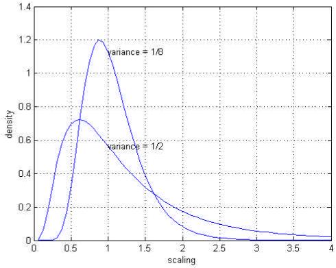
Log-normal densities: prior expectations of zero are shown with a variance of 1/2 and 1/8. These correspond to less informative and more informative priors respectively.

References

- Accardo A, Affinito M, Carrozzi M, Bouqet F. Use of fractal dimension for the analysis of electroencephalographic time series. Biol. Cybern. 1997;77:339–350. doi: 10.1007/s004220050394. [DOI] [PubMed] [Google Scholar]
- Barlow JS. The Electroencephalogram, Its Patterns and Origins. MIT Press; 1993. (1993) ISBN 0262023547. [Google Scholar]
- Barrie JM, Freeman WJ, Lenhart MD. Spatiotemporal analysis of prepyriform, visual, auditory and somethetic surface EEGs in trained rabbits. J. Neurophysiol. 1996;76(1):520–539. doi: 10.1152/jn.1996.76.1.520. 1996. [DOI] [PubMed] [Google Scholar]
- Benda J, Herz AV. A Universal Model for Spike-Frequency Adaptation. Neural Computation. 2003;15:2523–2564. doi: 10.1162/089976603322385063. [DOI] [PubMed] [Google Scholar]
- Brady AT, De Souza IEJ, O’Keeffe MA, Kenny CM, McCabe O, Moran MP, Duffy AM, Mulvany SK, O’Connor WT. Hypoglutamatergia in the rat medial prefrontal cortex in two models of schizophrenia. Acta Neurobiologiae Experimentalis. 2005;65:29. [Google Scholar]
- Breakspear M, Roberts JA, Terry JR, Rodrigues S, Mahant N, Robinson PA. A unifying explanation of primary generalized seizures through nonlinear brain modeling and bifurcation analysis. Cereb Cortex. 2006;16(9):1296–313. doi: 10.1093/cercor/bhj072. [DOI] [PubMed] [Google Scholar]
- Buzsaki G. Theta Oscillations in the Hippocampus. Neuron. 2002;33(3):325–340. doi: 10.1016/s0896-6273(02)00586-x. [DOI] [PubMed] [Google Scholar]
- Chichilnisky EJ. A simple white noise analysis of neuronal light responses. Comp in Neural Systems. 2001;12(2):199–213. [PubMed] [Google Scholar]
- David O, Harrison L, Friston KJ. Modelling event-related responses in the brain. NeuroImage. 2005;25(3):756–770. doi: 10.1016/j.neuroimage.2004.12.030. [DOI] [PubMed] [Google Scholar]
- David O, Kilner JM, Friston KJ. Mechanisms of evoked and induced responses in MEG/EEG. NeuroImage. 2006 Jul 15;31(4):1580–91. doi: 10.1016/j.neuroimage.2006.02.034. [DOI] [PubMed] [Google Scholar]
- David O, Harrison L, Friston KJ. Modelling event-related responses in the brain. NeuroImage. 2005 Apr 15;25(3):756–70. doi: 10.1016/j.neuroimage.2004.12.030. [DOI] [PubMed] [Google Scholar]
- David O, Cosmelli D, Friston KJ. Evaluation of different measures of functional connectivity using a neural mass model. NeuroImage. 2004 Feb;21(2):659–73. doi: 10.1016/j.neuroimage.2003.10.006. [DOI] [PubMed] [Google Scholar]
- David O, Friston KJ. A neural mass model for MEG/EEG: coupling and neuronal dynamics. NeuroImage. 2003 Nov;20(3):1743–55. doi: 10.1016/j.neuroimage.2003.07.015. [DOI] [PubMed] [Google Scholar]
- De Souza IEJ, Brady AT, O’Keeffe MA, Kenny CM, McCabe O, Moran MP, Duffy AM, Fitzgerald C, Mulvany SK, O’Connor WT. Effect of environment and clozapine on basal and stimulated medial prefrontal GABA release in two rat models of schizophrenia. Acta Neurobiologiae Experimentalis. 2005;65:40. [Google Scholar]
- Dumont M, Macchi MM, Carrier J, Lafrance C, Herbert M. Time course of narrow frequency bands in the waking EEG during sleep deprivation. NeuroReport. 1999;10(2):403–407. doi: 10.1097/00001756-199902050-00035. [DOI] [PubMed] [Google Scholar]
- Faber LES, Sah P. Calcium-Activated Potassium Channels: Multiple Contributions to Neuronal Function. The Neuroscientist. 2003;9(3):181–194. doi: 10.1177/1073858403009003011. [DOI] [PubMed] [Google Scholar]
- Friston KJ, Mattout J, Trujilo-Barreto N, Ashburner J, Penny W. Variational free energy and the Laplace approximation. NeuroImage. 2006;34:220–234. doi: 10.1016/j.neuroimage.2006.08.035. [DOI] [PubMed] [Google Scholar]
- Friston KJ, Glaser DE, Henson RNA, Kiebel S, Phillips C, Ashburner J. Classical and Bayesian Inference in Neuroimaging: Applications. NeuroImage. 2002;16:484–512. doi: 10.1006/nimg.2002.1091. [DOI] [PubMed] [Google Scholar]
- Friston KJ, Stephan KE, Lund TE, Morcom A, Kiebel S. Mixed-effects and fMRI studies. NeuroImage. 2005;24:244–252. doi: 10.1016/j.neuroimage.2004.08.055. [DOI] [PubMed] [Google Scholar]
- Fellous JM, Sejnowski J. Cholinergic Induction of Oscillations in the Hippocampal Slice in the Slow (0.5-2Hz), Theta (5-12), and Gamma (35-70) Bands. Hippocampus. 2000;10:187–197. doi: 10.1002/(SICI)1098-1063(2000)10:2<187::AID-HIPO8>3.0.CO;2-M. [DOI] [PubMed] [Google Scholar]
- Fellemann DJ, Van Essen DC. Distributed Hierarchical Processing in the Primate Cerebral Cortex. Cerebral Cortex. 1991;1(1):1–47. doi: 10.1093/cercor/1.1.1-a. [DOI] [PubMed] [Google Scholar]
- Fenton GW, Fenwick PB, Dollimore J, Dunn Tolland Hirsch SR. EEG spectral analysis in schizophrenia. The British Journal of Psychiatry. 1999;136:445–455. doi: 10.1192/bjp.136.5.445. 1980. [DOI] [PubMed] [Google Scholar]
- Freeman WJ. Linear analysis of the dynamics of neural masses. Ann. Rev. Biophys. Bioeng. 1972;1:225–256. doi: 10.1146/annurev.bb.01.060172.001301. [DOI] [PubMed] [Google Scholar]
- Gegelashvili G, Schouboe A. High Affinity Glutamate Transporters: Regulation of Expression and Activity. Molecular Pharmacology. 1997;52:6–15. doi: 10.1124/mol.52.1.6. [DOI] [PubMed] [Google Scholar]
- Geyer MA, Wilkinson LS, Humby T, Robbins TW. Isolation rearing of rats produces a deficit in prepulse inhibition of acoustic startle similar to that in schizophrenia. Biological Psychiatry. 1993:361–372. doi: 10.1016/0006-3223(93)90180-l. 34. [DOI] [PubMed] [Google Scholar]
- Geyer MA, Krebs-Thomson K, Braff DL. Swerdlow, Pharmacological studies of prepulse inhibition models of sensorimotor gating deficits in schizophrenia: a decade in review. Psychopharmacology. 2001;156(2-3) doi: 10.1007/s002130100811. [DOI] [PubMed] [Google Scholar]
- Hald LA, Bastiaansen CM, Hagoort P. EEG theta and gamma responses to semantic violations in online sentence processing. Brain and Language. 2006;96:90–105. doi: 10.1016/j.bandl.2005.06.007. [DOI] [PubMed] [Google Scholar]
- Hasselmo ME, Bodelon C, Wyble BP. A proposed function for hippocampal theta rhythm: Separate phases of encoding and retrieval enhance reversal of prior learning. Neural Computation. 2002;14(4):793–817. doi: 10.1162/089976602317318965. [DOI] [PubMed] [Google Scholar]
- Hertz L, Dringen R, Schousboe, Robinson SR. Astrocytes: Glutamate Producers for Neurons. Journal of Neuroscience Research. 1999;57:417–428. [PubMed] [Google Scholar]
- Hornero R, Alonso A, Jimeno N, Jimeno A, Lopez M. Nonlinear Analysis of Time Series Generated by Schizophrenic Patients. IEEE ENGINEERING IN MEDICINE AND BIOLOGY magazine. 1999 May;:0739–5175. doi: 10.1109/51.765193. [DOI] [PubMed] [Google Scholar]
- Hughes JR, John ER. Conventional and Quantitative Electroencephalography in Psychiatry. J Neuropsychiatry Clin Neurosci. 1999 May;11:190–208. doi: 10.1176/jnp.11.2.190. 1999. [DOI] [PubMed] [Google Scholar]
- Ishiwari K, Mingote S, Correa M, Trevitt JT, Carlson BB, Salamone JD. The GABA uptake inhibitor Beta-alanine reduces pilocarpine-induced tremors and increases extracellular GABA in substantia nigra pars reticulate as measured by microdialysis. Journal of Neuroscience Methods. 2004;140:39–46. doi: 10.1016/j.jneumeth.2004.03.030. [DOI] [PubMed] [Google Scholar]
- Jabaudon D, Shimamoto K, Yasuda-Kamatani Y, Scanziani M, Gahwiler BH, Gerber U. Inhibition of uptake unmasks rapid extracellular turnover of glutamate of nonvesicular origin. PNSA. 1999 Feb;96:8733–8738. doi: 10.1073/pnas.96.15.8733. [DOI] [PMC free article] [PubMed] [Google Scholar]
- Jansen BH, Rit VG. Electroencephalogram and visual evoked potential generation in a mathematical model of coupled cortical columns. Biological Cybernetics. 1995;(73):357–366. doi: 10.1007/BF00199471. 1995. [DOI] [PubMed] [Google Scholar]
- Jansen BH, Zouridakis G, Brandt ME. A neurophysiologically-based mathematical model of flash visual evoked potentials. Biol Cybernetics. 1993;68(3) doi: 10.1007/BF00224863. [DOI] [PubMed] [Google Scholar]
- Jensen O, Vanni S. A New Method to Identify Multiple Sources of Oscillatory Activity from Magnetoencephalographic Data. NeuroImage. 2002;15:568–574. doi: 10.1006/nimg.2001.1020. [DOI] [PubMed] [Google Scholar]
- Jirsa VK, Haken H. Field Theory of Electromagnetic Brain Activity. Phys Rev Lett. 1996;77(5):960–963. doi: 10.1103/PhysRevLett.77.960. [DOI] [PubMed] [Google Scholar]
- Kavalali ET, Plummer MR. Selective potentiation of a novel calcium channel in rat hippocampal neurones. J. Physiol. 1994;480:475–484. doi: 10.1113/jphysiol.1994.sp020376. [DOI] [PMC free article] [PubMed] [Google Scholar]
- Kavalali ET, Plummer MR. Multiple voltage-dependent mechanisms potentiate calcium channel activity in hippocampal neurons. J. Neurosci. 1996;16:1072–1082. doi: 10.1523/JNEUROSCI.16-03-01072.1996. [DOI] [PMC free article] [PubMed] [Google Scholar]
- Kiebel SJ, David O, Friston KJ. Dynamic causal modelling of evoked responses in EEG/MEG with lead field parameterization. NeuroImage. 2006 May;30(4):1273–1284. doi: 10.1016/j.neuroimage.2005.12.055. [DOI] [PubMed] [Google Scholar]
- Liley DT, Bojak I. Understanding the transition to seizure by modeling the epileptiform activity of general anesthetic agents. J Clin Neurophysiol. 2005 Oct;22(5):300–13. [PubMed] [Google Scholar]
- Lopes da Silva F. Neural mechanisms underlying brain waves: from neural membranes to networks. Electroencephalogr Clin Neurophysiol. 1991;79(2):81–93. doi: 10.1016/0013-4694(91)90044-5. [DOI] [PubMed] [Google Scholar]
- McLennan H. The effect of decortication on the excitatory amino acid sensitivity of striatal neurones. Neurosci Lett. 1980;18:313–316. doi: 10.1016/0304-3940(80)90303-1. [DOI] [PubMed] [Google Scholar]
- Mattout J, Phillips C, Penny WD, Rugg MD, Friston KJ. MEG source localization under multiple constraints: An extended Bayesian framework. NeuroImage. 2005;30(3):753–767. doi: 10.1016/j.neuroimage.2005.10.037. [DOI] [PubMed] [Google Scholar]
- Moran RJ, Kiebel SJ, Stephan KE, Reilly RB, Daunizeau J, Friston KJ. A Neural Mass Model of spectral responses in electrophysiology. NeuroImage. 2007;37(3):706–720. doi: 10.1016/j.neuroimage.2007.05.032. [DOI] [PMC free article] [PubMed] [Google Scholar]
- Oliet SHR, Piet R, Poulain DA. Control of Glutamate Clearance and synaptic Efficacy by Glial Coverage of Neurons. Science. 2001;292:923. doi: 10.1126/science.1059162. [DOI] [PubMed] [Google Scholar]
- Polich J, Pitzer A. P300 in early Alzheimer’s disease: Oddball task difficulty and modality effects. In: Comi G, Lucking CH, Kimura J, Rossini RM, editors. Clinical Neurophysiology: From Receptors to Perception, EEG Supplement. Elsevier; Amsterdam: 1999. pp. 281–287. [PubMed] [Google Scholar]
- Press WH, Teukolsky SA, Vetterling WT, Flannery BP. Numerical Recipes in C. Cambridge Univ. Press; Cambridge MA, USA: 1992. 1992. [Google Scholar]
- Riera J, Aubert E, Iwata K, Kawashima R, Wan X, Ozaki T. Fusing EEG and fMRI based on a bottom-up model: inferring activation and effective connectivity in neural masses. Philos Trans R Soc Lond B Biol Sci. 2005;360(1457):1025–41. doi: 10.1098/rstb.2005.1646. [DOI] [PMC free article] [PubMed] [Google Scholar]
- Robinson PA. Propagator theory of brain dynamics. Phys Rev E Stat Nonlin Soft Matter Phys. 2005 Jul;72(1 Pt 1):011904. doi: 10.1103/PhysRevE.72.011904. [DOI] [PubMed] [Google Scholar]
- Rowe DL, Robinson PA, Gordon E. Stimulant drug action in attention deficit hyperactivity disorder (ADHD): inference of neurophysiological mechanisms via quantitative modelling. Clin Neurophysiol. 2005 Feb;116(2):324–35. doi: 10.1016/j.clinph.2004.08.001. [DOI] [PubMed] [Google Scholar]
- Sanchez-Vives MV, Nowak LG, McCormick DA. Cellular mechanisms of long-lasting adaptation in visual cortical neurons in vitro. J. Neurosci. 2000;20:4286–4299. doi: 10.1523/JNEUROSCI.20-11-04286.2000. [DOI] [PMC free article] [PubMed] [Google Scholar]
- Seidenbecher T, Laxmi TR, Stork O, Pape HC. Amygdalar and hippocampal theta rhythm synchronization during fear memory retrieval. Science. 2003;301:846–850. doi: 10.1126/science.1085818. [DOI] [PubMed] [Google Scholar]
- Stephan KE, Baldeweg T, Friston KJ. Synaptic plasticity and dysconnection in schizophrenia. Biological Psychiatry. 2006;59:929–939. doi: 10.1016/j.biopsych.2005.10.005. [DOI] [PubMed] [Google Scholar]
- Tanaka H, Koenig T, Pascual-Marqui RD, Hirata K, Kochi K, Lehmann D. Event-Related Potential and EEG Measures in Parkinson’s Disease without and with Dementia. Dementia and Geriatric Cognitive Disorders. 2000;11:39–45. doi: 10.1159/000017212. 2000. [DOI] [PubMed] [Google Scholar]
- Timmerman W, Westerink BHC. Brain Microdialysis of GABA and Glutamate: What Does it Signify? Synapse. 1997;27:242–261. doi: 10.1002/(SICI)1098-2396(199711)27:3<242::AID-SYN9>3.0.CO;2-D. [DOI] [PubMed] [Google Scholar]
- Traub RD, Whittington MA, Stanford IM, Jefferys JGR. A mechanism for the generation of long-range synchronous fast oscillations in the cortex. Nature. 1996;383:621–624. doi: 10.1038/383621a0. [DOI] [PubMed] [Google Scholar]
- Wendling F, Bellanger JJ, Bartolomei F, Chauvel P. Relevance of nonlinear lumped-parameter models in the analysis of depth-EEG epileptic signals. Biological Cybernetics. 2000 Sep;8(4):367–378. doi: 10.1007/s004220000160. [DOI] [PubMed] [Google Scholar]
- Wright JJ, Liley DT. A millimetric-scale simulation of electrocortical wave dynamics based on anatomical estimates of cortical synaptic density. Computation in Neural Systems. 1994;5(2):191–202. [Google Scholar]
- Van Den Pol AN, Obrietan K, Belousov A. Glutamate hyperexcitability and seizure-like activity throughout the brain and spinal cord upon relief from chronic glutamate receptor blockade in culture. Neuroscience. 1996;74:653–674. doi: 10.1016/0306-4522(96)00153-4. [DOI] [PubMed] [Google Scholar]
- Vida I, Bartos M, Jonas P. Shunting inhibition improves robustness of Gamma Oscillations in Hippocampal Interneuron Networks by Homogenizing Firing Rates. Neuron. 2006;49(1):107–117. doi: 10.1016/j.neuron.2005.11.036. [DOI] [PubMed] [Google Scholar]
- Vinogradova OS. Expression, control and probable functional significance of the neuronal theta-rhythm. Prog Neurobiol. 1995;45(6):523–583. doi: 10.1016/0301-0082(94)00051-i. [DOI] [PubMed] [Google Scholar]