Investigating the functional role of callosal connections with dynamic causal models

Abstract

The anatomy of the corpus callosum has been described in considerable detail. Tracing studies in animals and human post-mortem experiments are currently complemented by diffusion-weighted imaging, which enables non-invasive investigations of callosal connectivity to be conducted. In contrast to the wealth of anatomical data, little is known about the principles by which inter-hemispheric integration is mediated by callosal connections. Most importantly, we lack insights into the mechanisms that determine the functional role of callosal connections in a context-dependent fashion. These mechanisms can now be disclosed by models of effective connectivity that explain neuroimaging data from paradigms which manipulate inter-hemispheric interactions. In this article, we demonstrate that Dynamic Causal Modeling (DCM), in conjunction with Bayesian model selection (BMS), is a powerful approach to disentangling the various factors that determine the functional role of callosal connections. We first review the theoretical foundations of DCM and BMS before demonstrating the application of these techniques to empirical data from a single subject.

Introduction

Ever since the description of localizable lesion and excitation effects in the 19^th century, modern neuroscience has revolved around the twin themes of functional specialization and functional integration^1,2. Functional specialization refers to the notion that local neural units are specialized in certain aspects of information processing, e.g. the processing of particular stimulus properties. Traditional methods for investigating functional specialization include invasive recordings from animals and neuropsychological investigations of patients with brain lesions. More recently, functional neuroimaging techniques like functional magnetic resonance imaging (fMRI) have made it possible to investigate functional specialization across the whole brain in a non-invasive manner. In contrast, functional integration refers to the causal interactions among distinct neural units. Critically, the form of these causal interactions, which mediate complex cognitive processes, is constrained by the anatomical connections between the neural units. Consequently, in order to understand the basis of functional integration, much effort has been invested in characterizing anatomical connectivity in the mammalian brain. For example, thousands of tract tracing experiments have been performed in several species over the last decades. These techniques require the in vivo injection of specific dyes into particular areas. Depending on its biophysical properties, the dye is taken up by neuronal somata or axonal terminals and transported in an anterograde or retrograde direction, respectively³. Subsequent histological processing of the brain can then reveal the regions that receive connections from (anterograde tracer) or send connections to (retrograde tracer) the injected area. For the Macaque monkey alone, more than 36,000 individual experimental findings from tracing experiments are described by the connectivity database CoCoMac⁴ (see www.cocomac.org).

Unfortunately, for the human brain we have considerably less knowledge about its anatomical connections. This is because tract tracing procedures, as the gold-standard method to reveal anatomical connections, are too invasive to use in the human brain. There has been an intensive search for post mortem methods as an alternative to investigate human brain connectivity, but these methods are either restricted to very large fibre bundles⁵ or limited to very short intra-cortical connections⁶.

Recently, the advent of noninvasive diffusion-weighted imaging (DWI) techniques, e.g. diffusion tensor imaging (DTI), has raised great hopes that we may be able to obtain a complete picture of human brain connectivity in the not too distant future. However, the resolution of current DWI approaches is still too coarse to allow for characterizations that are comparable to those obtained from tracing techniques, and fundamental problems like intra-voxel fiber crossings still need to be solved convincingly. Using improved acquisition schemes, probabilistic approaches^7,8 and models that do not make strong a priori assumptions about the shape of the spatial distribution of diffusion⁹, these technical limitations might eventually be overcome. Should this indeed be possible, would this mean that we have all the information we need to understand principles of functional integration in the human brain? The answer is, unfortunately, no. Even if we knew everything about the anatomical connectivity of a particular neural system, we cannot directly derive its dynamics from its connectional structure¹⁰. Further knowledge is required, for example of the time constants of activity propagation or the strength of individual connections and how these change as a function of cognitive context (task requirements, learning, etc)¹¹. These time constants and connection strengths are parameters that have to be estimated from empirical observations. In conclusion, knowledge of anatomical connectivity is a necessary, but not sufficient, condition to build dynamical models of brain function.

One good example is the corpus callosum. This massive fiber bundle, which contains a huge number of axons that link and functionally integrate the two hemispheres, has been investigated in great detail. We know the source and target laminae of neurons projecting through the corpus callosum¹², the spatial distribution of axonal diameters across the callosum¹³, and the topography of individual callosal projections^14,15. Neuropsychological studies have demonstrated the involvement of very restricted parts of the corpus callosum in specific cognitive processes¹⁶. More recently, the corpus callosum has been studied intensively by DWI studies that have investigated its connectivity both in healthy subjects¹⁷ and patients¹⁸. Yet, in spite of all these data, we still lack any powerful theory of callosal function and how it underlies inter-hemispheric integration. Banich and colleagues have recently advanced a useful framework that relates the functional role of the corpus callosum to the complexity of cognitive tasks and attentional processing¹⁹, but this theory is neither quantitative nor directly embedded into a precise neurobiological model.

An important starting point for more precise theories of callosal function would be to investigate neurobiologically plausible models of inter-hemispheric integration in order to (i) identify those cognitive factors that determine the functional role of specific callosal connections, (ii) determine, quantitatively, the strength of callosal connections as a function of experimentally controlled cognitive context, and (iii) analyze the pattern of context-dependent connection strengths with regard to interesting features, e.g. directional asymmetries or differences in modulation by different cognitive factors. Models of effective connectivity, which are based on empirical neuroimaging data and model the modulation of connection strengths by experimentally controlled changes in context, would be ideal to do this. Previously available techniques for studying effective connectivity, for example structural equation modeling (SEM), are not well suited for models of high connectional complexity, e.g. multiple reciprocal connections and loops, due to potential problems of identifiability²⁰. This is a particular problem for models of inter-hemispheric integration because callosal connections appear to be generally reciprocal between homotopic regions^21,22. Furthermore, SEM operates at the level of measured hemodynamic responses and does not offer a model of the underlying neural processes.

In this article, we demonstrate how a novel method to study effective connectivity, Dynamic Causal Modeling (DCM¹¹), can be combined with Bayesian model selection (BMS²³) to address quite complex questions about callosal function. First, we briefly review the theoretical foundations of both DCM and BMS. Subsequently, we apply DCM to fMRI data from a single subject who performed a task that manipulated inter-hemispheric interactions. Specifically, we focus on the question of how competing hypotheses about the functional role of callosal connections in a specific cognitive context can be disambiguated using BMS.

Methods

Dynamic Causal Modeling

DCM is a method to make inferences about neural processes that underlie measured time series, in our case fMRI data. The general idea is to estimate the parameters of a reasonably realistic neuronal system model such that the predicted blood oxygen level dependent (BOLD) signal, which results from converting the modeled neural dynamics into hemodynamic responses, corresponds as closely as possible to the observed BOLD time series. As in state-space models, two distinct levels constitute a DCM (see Figure 1). The hidden level, which cannot be directly observed using fMRI, represents a simple model of neural dynamics in a system of k coupled brain regions. Each system element i is represented by a single state variable z_i, and the dynamics of the system is described by the change of the neural state vectorz z = [z₁,…, z_k]^T over time. The neural state variables do not correspond directly to any common neurophysiological measurement (such as spiking rates or local field potentials) but represent a summary index of neural population dynamics in the respective regions. Importantly, DCM models how the neural dynamics are driven by external perturbations that result from experimentally controlled manipulations. These perturbations are described by means of external inputs u that enter the model in two different ways: they can elicit responses through direct influences on specific regions (“driving” inputs, e.g. evoked responses in early sensory areas) or they can change the strength of coupling among regions (“modulatory” inputs, e.g. during learning or attention). Overall, DCM models the temporal evolution of the neural state vector, i.e. $\stackrel{.}{z}=\frac{\mathit{dz}}{\mathit{dt}}$, as a function of the current state, the inputs u and some parameters θⁿ that define the functional architecture and interactions among brain regions at a neuronal level (n is not an exponent but simply denotes “neural”):

$$\left[\begin{array}{c}\hfill {\stackrel{.}{z}}_1\hfill \\ \hfill ⋮\hfill \\ \hfill {\stackrel{.}{z}}_k\hfill \end{array}\right]=\stackrel{.}{z}=F(z,u,{\theta }^n)$$ (1)

In this neural state equation, the state z and the inputs u are time-dependent whereas the parameters are time-invariant. In DCM, F has the bilinear form

$$\stackrel{.}{z}=\mathit{Az}+\underset{j=1}{\overset{m}{\Sigma }}u{}_{j}B{}_{j}z+\mathit{Cu}$$ (2)

The parameters of this bilinear neural state equation, θⁿ = {A,B₁,…,B_m,C} can be expressed as partial derivatives of F:

$$\begin{array}{cc}\hfill A& =\frac{\partial F}{\partial z}=\frac{\partial \stackrel{.}{z}}{\partial z}\hfill \\ \hfill B_j& =\frac{{\partial }^{2}F}{\partial z\partial u_j}=\frac{\partial }{\partial u_j}\frac{\partial \stackrel{.}{z}}{\partial z}\hfill \\ \hfill C& =\frac{\partial F}{\partial u}\hfill \end{array}$$ (3)

These parameter matrices describe the nature of the three causal components which underlie the modeled neural dynamics: (i) context-independent effective connectivity among brain regions, mediated by anatomical connections (k×k matrix A), (ii) context-dependent changes in effective connectivity induced by the j^th input u_j (k×k matrices B₁,…B_m), and (iii) direct inputs into the system that drive regional activity (k×m matrix C). As will be demonstrated below, the posterior distributions of these parameters can inform us about the impact that different mechanisms have on determining the dynamics of the model. Notably, the distinction between “driving” and “modulatory” is neurobiologically relevant: driving inputs exert their effects through direct synaptic responses in the target area, whereas modulatory inputs change synaptic responses in the target area in response to inputs from another area. This distinction represents an analogy, at the level of large neural populations, to the concept of driving and modulatory afferents in studies of single neurons²⁴.

Figure 1.

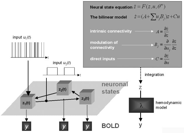
Schematic summary of the conceptual basis of DCM. The dynamics in a system of interacting neuronal populations (left lower panel), which are not directly observable by fMRI, is modeled using a bilinear state equation (right upper panel). Integrating the state equation gives predicted neural dynamics (z) that enter a model of the hemodynamic response (λ) to give predicted BOLD responses (y) (right lower panel). The parameters at both neural and hemodynamic levels are adjusted such that the differences between predicted and measured BOLD series are minimized. Critically, the neural dynamics are determined by experimental manipulations. These enter the model in the form of external inputs (left upper panel). Driving inputs (u₁; e.g. sensory stimuli) elicit local responses directly that are propagated through the system according to the intrinsic connections. The strengths of these connections can be changed by modulatory inputs (u₂; e.g. changes in cognitive set, attention, or learning). In this figure, the structure of the system and the scaling of the inputs are arbitrary.

DCM combines this model of neural dynamics with a biophysically plausible and experimentally validated hemodynamic model that describes the transformation of neuronal activity into a BOLD response. This so-called “Balloon model” was initially formulated by Buxton and colleagues²⁵ and later extended by Friston et al.^26,27. Briefly summarized, it consists of a set of differential equations that describe the relations between four hemodynamic state variables, using five parameters (θ^h). More specifically, changes in neural activity elicit a vasodilatory signal that leads to increases in blood flow and subsequently to changes in blood volume v and deoxyhemoglobin content q. The predicted BOLD signal y is a non-linear function of blood volume and deoxyhemoglobine content: y = λ(v​,q). Details of the hemodynamic model can be found in other publications^11,26,27.

By combining the neural and hemodynamic states into a joint state vector x and the neural and hemodynamic parameters into a joint parameter vector θ = [θⁿθ^h]^T, we obtain the full forward model that is defined by the neural and hemodynamic state equations

$$\begin{array}{cc}\hfill \stackrel{.}{x}& =F(x,u,\theta )\hfill \\ \hfill y& =\lambda \left(x\right)\hfill \end{array}$$ (4)

For any given set of parameters θ and inputs u, the joint state equation can be integrated and passed through the output nonlinearity λ to give a predicted BOLD response h(u,θ). This can be extended to an observation model that includes observation error ε and confounding effects X (e.g. scanner-related low-frequency drifts):

$$y=h(u,\theta )+X\beta +\epsilon$$ (5)

This formulation is the basis for estimating the neural and hemodynamic parameters from the measured BOLD data, using a fully Bayesian approach with empirical priors for the hemodynamic parameters and conservative shrinkage priors for the neural coupling parameters. Details of the parameter estimation scheme, which rests on a Gauss-Newton gradient ascent embedded in an expectation maximization (EM) algorithm, can be found elsewhere¹¹. In brief, under Gaussian assumptions about the posterior distributions (Laplace approximation), this scheme returns the posterior expectations (= maximum a posteriori [MAP] estimates) η_θ|y and posterior covariance C_θ|y for the parameters as well as hyperparameters for the covariance of the observation noise, C_ε.

After fitting the model to measured BOLD data, the posterior distributions of the parameters can be used to test hypotheses about the size and nature of effects at the neural level. Although inferences could be made about any of the parameters in the model, hypothesis testing usually concerns context-dependent changes in coupling (i.e. specific parameters from the B matrices). As will be demonstrated below, at the single-subject level, these inferences concern the question of how certain one can be that a particular parameter or, more generally, a contrast of parameters, C^Tη_θ|y, exceeds a particular threshold γ (e.g. zero; see Fig. 6). Under the assumptions of the Laplace approximation, this is easy to test (φ_N denotes the cumulative normal distribution):

$$p(c^T{\eta }_{\theta \mid y}>\gamma )={\varphi }_N\left(\frac{c^T{\eta }_{\theta \mid y}-\gamma }{\sqrt{c^T{C}_{\theta \mid y}c}}\right)$$ (6)

For example, for the special case C^Tη_θ|y = γ the probability is p(C^Tη_θ|y > γ) = 50%, i.e. it is equally likely that the parameter is smaller or larger than the chosen threshold γ. We conclude this section on the theoretical foundations of DCM by noting that the parameters can be understood as rate constants (units: 1/s = Hz) of neural population responses that have an exponential nature (see also Fig. 1 in ref. 28). This is easily understood if one considers that the solution to a linear ordinary differential equation of the form ż = Az is an exponential function (compare the state equation in Eq. 2).

Figure 6.

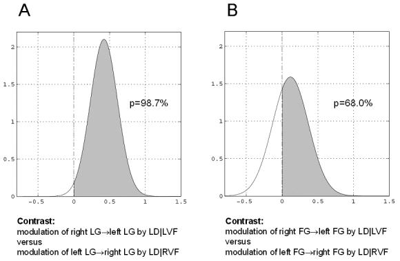
Asymmetry of callosal connections with regard to contextual modulation. The plots show the probability that the modulation of the right→left connection by task conditional on left visual field stimulation is stronger than the modulation of the left→right connection by task conditional on right visual field stimulation. A. For the callosal connections between left and right LG, we have can be very confident that this asymmetry exists: the probability of the contrast being larger than zero is p(c^Tη_θ|y > 0) = 98.7%. B. For the callosal connections between left and right FG, we are considerably less certain about the presence of this asymmetry: the probability of the contrast being larger than zero is p(c^Tη_θ|y > 0) = 68.0%.

Bayesian model selection

A generic problem encountered by any kind of modeling approach is the question of model selection: given some observed data, which of several alternative models is the optimal one? This problem is not trivial because the decision cannot be made solely by comparing the relative fit of the competing models. One also needs to take into account the relative complexity of the models as expressed, for example, by the number of free parameters in each model. Model complexity is important to consider because there is a trade-off between model fit and generalizability (i.e. how well the model explains different data sets that were all generated from the same underlying process). As the number of free parameters is increased, model fit increases monotonically whereas beyond a certain point model generalizability decreases. The reason for this is “overfitting”: an increasingly complex model will, at some point, start to fit noise that is specific to one data set and thus become less generalizable across multiple realizations of the same underlying generative process. (Generally, in addition to the number of free parameters, the complexity of a model also depends on its functional form²⁹. This is not an issue for DCM, however, because here all possible models have the same functional form.)

Therefore, the question “What is the optimal model?” can be reformulated more precisely as “What is the model that represents the best balance between fit and complexity?” In a Bayesian context, the latter question can be addressed by comparing the evidence, p(y|m), of different models. According to Bayes theorem

$$p(\theta \mid y,m)=\frac{p(y\mid \theta ,m)p(\theta \mid m)}{p(y\mid m)}$$ (7)

the model evidence can be considered as a normalization constant for the product of the likelihood of the data and the prior probability of the parameters, therefore

$$p(y\mid m)\int p(y\mid \theta ,m)p(\theta \mid m)d\theta$$ (8)

Here, the number of free parameters (as well as the functional form) are considered by the integration. Unfortunately, this integral cannot usually be solved analytically, therefore an approximation to the model evidence is needed.

In the context of DCM, one potential solution could be to make use of the Laplace approximation, i.e. to approximate the model evidence by a Gaussian that is centered on its mode. As shown by Penny et al.²³, this yields the following expression for the natural logarithm (ln) of the model evidence (η_θ|y denotes the MAP estimate, C_θ|y is the posterior covariance of the parameters, C_ε is the error covariance, θ_p is the prior mean of the parameters, and C_p is the prior covariance):

$$\begin{array}{cc}\hfill & \ln p(y\mid m)=\mathit{accuracy}\left(m\right)-\mathit{complexity}\left(m\right)\hfill \\ \hfill & =\left[-\frac{1}{2}\ln \left|C_{\epsilon }\right|-\frac{1}{2}{\left(y-h(u,{\eta }_{\theta \mid y}\right)}^T{C}_{\epsilon }^{-1}\left(y-h(u,{\eta }_{\theta \mid y}\right)\right]\hfill \\ \hfill & -\left[\frac{1}{2}\ln \left|C_p\right|-\frac{1}{2}\ln \left|C_{\theta \mid y}\right|+\frac{1}{2}{\left({\eta }_{\theta \mid y}-{\theta }_p\right)}^T{C}_p^{-1}\left({\eta }_{\theta \mid y})-{\theta }_p\right)\right]\hfill \end{array}$$ (9)

This expression properly reflects the requirement, as discussed above, that the optimal model should represent the best compromise between model fit (accuracy) and model complexity. The complexity term depends on the prior density, for example, the prior covariance of the intrinsic connections (see Eq. 9). This is problematic in the context of DCM for fMRI because this prior covariance is defined in a model-specific fashion to ensure that the probability of obtaining an unstable system is very small. (Specifically, this is achieved by choosing the prior covariance of the intrinsic coupling matrix A such that the probability of obtaining a positive Lyapunov exponent of A is p < 0.001; see Friston et al.¹¹ for details.) Consequently, one cannot easily compare models with different numbers of connections. Therefore, alternative approximations to the model evidence are useful for DCMs of this sort.

Suitable approximations, which do not depend on the prior density, are afforded by the Bayesian Information Criterion (BIC) and Akaike Information Criterion (AIC), respectively. As shown by Penny et al.²³, for DCM these approximations are given by

$$\begin{array}{cc}\hfill & \mathit{BIC}=\mathit{accuracy}\left(m\right)-\frac{d_{\theta }}{2}\ln N\hfill \\ \hfill & \mathit{AIC}=\mathit{accuracy}\left(m\right)-d_{\theta }\hfill \end{array}$$ (10)

where d_θ is the number of parameters and N is the number of data points (scans). If one compares the complexity terms of BIC and AIC, it becomes obvious that BIC pays a heavier penalty than AIC as soon as one deals with 8 or more scans (which is virtually always the case for fMRI data):

$$\begin{array}{cc}\hfill & \frac{d_{\theta }}{2}\ln N>d_{\theta }\hfill \\ \hfill & \Rightarrow N>e^2\approx 7.39\hfill \end{array}$$ (11)

Therefore, BIC will be biased towards simpler models whereas AIC will be biased towards more complex models. This can lead to disagreement between the two approximations about which model should be favored. We have therefore adopted the convention that, for any pairs of models m_i and m_j to be compared, a decision is only made if AIC and BIC concur; the decision is then based on that approximation which gives the smaller Bayes factor:

$${\mathit{BF}}_{\mathit{ij}}=\frac{p(y\mid m_i)}{p(y\mid m_j)}$$ (12)

This approach to BMS is a robust procedure to decide between competing hypotheses represented by different DCMs. These hypotheses can concern any part of the structure of the modeled system, e.g. the pattern of intrinsic connections or which inputs affect the system and where they enter. Below, we will show a concrete example that demonstrates how the combination of DCM and BMS can be applied in practice to disclose previously unknown principles of inter-hemispheric integration.

Some considerations on the study of inter-hemispheric integration

Inter-hemispheric integration appears to be an ongoing process that is invoked by any cognitive task and cannot be abolished voluntarily. The question for the experimentalist is therefore not how to induce or prevent inter-hemispheric integration, but rather how to alter the form it takes. Two experimental manipulations are particularly effective for so doing. First, there are various ways of delivering sensory stimuli such that one hemisphere is initially or preferentially affected by these stimuli. For example, due to the topography of the anatomical connections from the retina to the visual cortex, presentation of visual stimuli in the periphery of one visual hemifield ensures that the contralateral visual cortex receives the stimulus information first. Therefore, one knows that any area that is in the hemisphere ipsilateral to stimulus presentation can only receive this information if it is transferred through the corpus callosum (or some alternative, e.g. subcortical, commissure). Second, if one uses a strongly lateralized task that draws on easily identified areas, one knows the target hemisphere and the target areas that require the stimulus information.

Combining both approaches allows one to predict precisely where the stimulus information initially enters the system and to which areas of the system it must be transferred. The challenge is then to characterize the potential paths of information flow and how these pathways are modulated by cognitive context. Rephrasing the question about the nature of inter-hemispheric integration in this way shows that we are dealing with a generic system identification problem which, in the context of neuroimaging, is best addressed using models of effective connectivity^1,30. Unfortunately, very few neuroimaging studies have been conducted so far that directly tackle the question of inter-hemispheric integration on the basis of a precisely defined system model (see McIntosh et al.³¹ for an exception).

In the next sections, we will provide an example for using DCM and BMS to address the mechanisms underlying inter-hemispheric integration. This example focuses on the ventral stream of the visual system and is motivated by a recent study that combined the two experimental manipulations described above, i.e. using two strongly and inversely lateralized tasks operating on identical visual stimuli that were presented peripherally in the visual hemifields³².

Inter-hemispheric integration in the ventral stream of the visual system

In a previous fMRI study on the mechanisms underlying hemispheric specialization, we investigated whether lateralization of brain activity depends on the nature of the sensory stimuli or on the nature of the cognitive task performed³². For example, microstructural differences between homotopic areas in the left and right hemisphere have been reported, including visual³³ and language-related³⁴ areas. Within a given hemisphere, these differences could favor the processing of certain stimulus characteristics and disadvantage others and might thus support stimulus-dependent lateralization in a bottom-up fashion³⁵. On the other hand, processing demands, mediated through cognitive control processes, might determine in a top-down fashion which hemisphere obtains precedence in a particular task context^36,37. To decide between these two possibilities, we used a paradigm in which the stimuli were kept constant throughout the experiment, and subjects were alternately instructed to attend to certain stimulus features and ignore others³². The stimuli were concrete German nouns (each four letters in length) in which either the second or third letter was printed in red (the other letters were black). In a letter decision (LD) task, the subjects had to ignore the position of the red letter and indicate whether or not the word contained the target letter “A”. In a spatial decision (SD) task they were required to ignore the language-related properties of the word and to judge whether the red letter was located left or right of the word centre. 50% of the stimuli were presented in the non-foveal part of the right visual field (RVF) and the other 50% in the non-foveal part of the left visual field (LVF).

The results of a conventional fMRI data analysis were clearly in favor of the top-down hypothesis: despite the use of identical word stimuli in all conditions, comparing spatial to letter decisions showed strongly right-lateralized activity in the parietal cortex, whereas comparing letter to visuospatial decisions showed strongly left-lateralized activity, including classical language areas in the left inferior frontal gyrus and visual areas in the left ventral visual stream, e.g. in the fusiform gyrus (FG), middle occipital gyrus (MOG) and lingual gyrus (LG) (see Figure 2).

Figure 2.

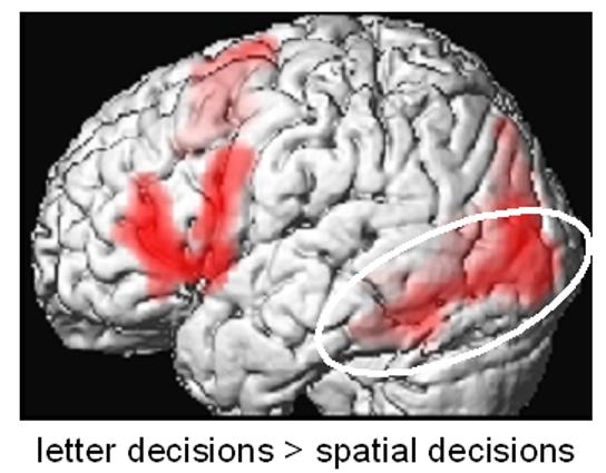
Results from a conventional analysis of the fMRI data by Stephan et al.³¹ using SPM99. Comparing letter decisions to visuospatial decisions about identical stimuli showed strongly left-lateralized activity, including classical language areas in the left inferior frontal gyrus and visual areas in the left ventral visual stream (white ellipse), e.g. in the fusiform gyrus, middle occipital gyrus and lingual gyrus. Results are shown at p<0.05, corrected at the cluster level for multiple comparisons across the whole brain. Adapted, with permission, from Figure 1 in ref. 31.

We now want to demonstrate how one can use DCM to investigate inter-hemispheric interactions with this paradigm. We focus on the ventral stream of the visual system which, as shown in Fig. 2, is preferentially involved in letter decisions in this experiment. For simplicity, we initially omit MOG and concentrate on LG and FG. First, we need to define a model comprising these four areas (Fig. 3A). To start with the direct (driving) inputs to the system, we model the lateral stimulus presentation and the crossed course of the visual pathways by allowing all RVF stimuli to directly affect left LG activity and all LVF stimuli to directly affect right LG activity, regardless of task. Each stimulus lasted for 150 ms only, therefore these inputs are represented as trains of short events (delta functions). The induced activity then spreads through the system according to the intrinsic connections of the model. For visual areas, it is biologically plausible to assume that both the intra- and the inter-hemispheric connections are reciprocal and that homotopic regions in both hemispheres are linked by inter-hemispheric connections^{14,21,22,38,39}.

Figure 3.

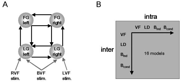
A. Basic structure of a model that comprises the left and right lingual gyrus (LG) and left and right fusiform gyrus (FG). The areas are reciprocally connected (black arrows). Driving inputs are shown as gray arrows. RVF stimuli directly affect left LG activity and LVF stimuli directly affect right LG activity, regardless of task context. Individual stimuli lasted for 150 ms only, therefore these inputs are represented as trains of events (delta functions). During the instruction periods, bilateral visual field input was provided for 6 s; this was modeled as a box-car input affecting LG in both hemispheres.

B. Schema showing how the 16 models tested were constructed by systematically combining four different types of modulatory inputs for inter- and intra-hemispheric connections; these different inputs are described by Figure 4.

Note that up to this point there are few, if any, plausible alternatives for how a DCM of inter-hemispheric integration between LG and FG, respectively, should be constructed. The important question, however, is how transcallosal information transfer is regulated by cognitive set. For example, one could assume that the strengths of inter-hemispheric interactions between visual areas are merely determined by the visual field of stimulus presentation, regardless of what the subject is instructed to do with the stimulus: whenever a stimulus is presented in the LVF, for example, and stimulus information is thus received initially by the right visual cortex, this information is transmitted transcallosally to the left visual cortex. Vice versa, whenever a stimulus is presented in the RVF, stimulus information is transmitted transcallosally from left to right visual cortex. In this scenario, the task performed is assumed to have no influence on callosal couplings. In contrast to this notion, results from previous analyses of these data by simple models of effective connectivity have indicated the importance of task demands on modulating functional couplings within hemispheres³². If this finding extends to inter-hemispheric interactions, one might expect that callosal connection strengths depend more on which task is performed than on which visual field the stimulus is presented in. That is, both right→left and left→right callosal connections could be enhanced during the letter decision task, enabling a tight cooperation of the two hemispheres during the task. As a third hypothesis, it is conceivable that both visual field and task exert an influence on callosal connection strengths, but independently of each other. As a fourth and final option, one might postulate that task demands modulate callosal connections, but conditional on the visual field, i.e. right→left connections are only modulated by LD during LVF stimulus presentation (LD|LVF) whereas left→right connections are only modulated by LD during RVF stimulus presentation (LD|RVF).

Each of these hypotheses of how cognitive set may modulate the callosal connections represents a different DCM, describing the mechanisms that caused the observed data. This model selection problem can be addressed by means of BMS. Briefly summarized, the four competing hypotheses are the following (see Figure 4A):

• (i) Information transfer between hemispheres depends only on the visual field of stimulus presentation. This is referred to as the VF model.

• (ii) Information transfer between hemispheres depends only on whether the letter decision task is performed or not. This is the LD model.

• (iii) Information transfer between hemispheres depends on both the task and the visual field, but independently of each other (corresponding to a Boolean OR operation). This is the B_ind model.

• (iv) Information transfer between hemispheres depends on both the task and the visual field, but in a conditional fashion: modulation of connection strength by task is only present if the stimulus was presented in a particular visual field (corresponding to a Boolean AND operation). This is the B_cond model.

Although less interesting in the present context, the same questions about the nature of modulatory inputs arise with respect to the intra-hemispheric connections. Therefore, to perform a thorough model comparison, one needs to systematically compare all combinations how inter- and intra-hemispheric connections are changed in the four ways described above (note that in the models presented here, we only allowed for modulation of the intra-hemispheric connections from LG→FG but not from FG→LG; see Fig. 4B). Figure 3B summarizes the combinatorial logic that resulted in 16 different models which were fitted to the same data. In the following we refer to these 16 models by first listing the modulation of the inter- and then that of the intra-hemispheric connections. For example, LD-VF is the model where the callosal connections are modulated by the letter decision task and the intra-hemispheric connections are modulated by the visual field. Once the best model and thus the factors that most strongly determine transcallosal information transfer in the context of the present task are identified, we can use the posterior density of the parameters of that model to characterize mechanisms of inter-hemispheric interactions. For example, we can attempt to clarify at what stage of the ventral stream contextual modulation of callosal connections is present. With the exception of some EEG studies^40,41, which have rather low spatial resolution, this is a largely unexplored issue. Of even more interest, however, is whether the contextual modulation of callosal connections is asymmetric, i.e. stronger for right→left connections than left→right connections or vice versa, and whether this asymmetry generalizes across the visual system or is specific to particular connections. This is a new dimension of hemispheric asymmetry that goes beyond the classical characterization of hemispheric specialization in terms of lateralized local activations and is directly related to the functional role of individual callosal “channels”.

Figure 4.

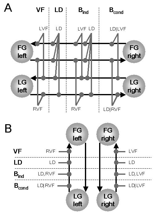
This figure describes four competing hypotheses about which experimental factors determine the strength of inter-hemispheric connections (A) and intra-hemispheric connections (B), respectively. These different types of modulatory inputs were combined to give 16 different models (compare Figure 3B). In contrast to the driving inputs (Fig. 3A), which were modeled as streams of events, all modulatory inputs were modeled as extended processes, i.e. box-car inputs of 24 s duration.

Results

Here we report the results from fitting the 16 DCMs described above to the fMRI data of a single subject from the study by Stephan et al.³². We initially present a four-area model as shown in Fig. 3, i.e. comprising bilateral LG and FG, and subsequently extend the model to include the MOG in both hemispheres.

Starting with the four-area case, the BMS procedure indicated that, for the particular subject studied, the model that represented the best balance between model fit and model complexity was the B_cond-LD model, i.e. modulation of inter-hemispheric connections by the letter decision task conditional on the visual field of stimulus presentation and modulation of intra-hemispheric connection strengths by the task only. Table 1 shows the Bayes factors for the comparison of the B_cond-LD model with the other 15 models. The AIC and BIC approximations agreed for all comparisons. The second-best model was the LD-B_cond model (i.e. the “flipped” version of the B_cond-LD model). The Bayes factor of comparing the B_cond-LD with the LD-B_cond model was only 2.33 which, according to the criteria summarized by Penny et al.²² (see their table 1), could be interpreted as weak evidence in favor of the B_cond-LD model. All other comparisons gave Bayes factors larger than 3, representing positive, strong or very strong evidence in favor of the B_cond-LD model (see Table 1).

Table 1.

This table shows the Bayes factors (middle column) for the comparison of the best model (B_cond-LD) with each of the other 15 models (left column). The right column lists the interpretation of the evidence in favor of the B_cond-LD model according to the criteria summarized by Penny et al.²³ (see their table 1).

Bcond-LD vs.	BF	evidence in favor of Bcond-LD
Bind-Bind	477.31	very strong
Bind-Bcond	60.83	strong
Bind-LD	110.84	strong
Bind-VF	479.03	very strong
Bcond-Bind	3.92	positive
Bcond-Bcond	4.48	positive
Bcond-VF	46267.47	very strong
LD-Bind	19.96	positive
LD-Bcond	2.33	weak
LD-LD	3.43	positive
LD-VF	29.74	strong
VF-Bind	16.85	positive
VF-Bcond	4.81	positive
VF-LD	5.59	positive
VF-VF	1.35E+13	very strong

Figure 5 shows the MAP estimates of the modulatory parameters (± standard deviation, i.e. the square root of the posterior variances) for the B_cond-LD model. The numerical values of the modulatory parameter estimates indicated an obvious hemispheric asymmetry: both at the levels of LG and FG, the MAP estimates of the modulation of the right→left connections are much larger than those of the left→right connections. But how secure is our inference about this asymmetry? This issue can be addressed by means of contrasts of the appropriate parameter estimates. The contrasts comparing modulation of the right→left connection by LD|LVF versus modulation of the left→right connection by LD|RVF are shown in Figure 6 (separately for connections at the levels of LG and FG, respectively). These plots indicate our certainty about asymmetrical modulation of callosal interactions through the probability that these contrasts exceed a value of zero (see Eq. 6). For the particular subject shown here, we can be very certain (98.7%) that modulation of the right LG→left LG connection by LD|LVF (0.34 ± 0.14 Hz) is larger than the modulation of the left LG→right LG connection by LD|RVF (−0.08 ± 0.16 Hz) (compare Figs. 4, 5). Although there is also a clear difference in the MAP estimates of the modulatory parameters of the callosal connections at the level of the FG, the difference is smaller and the variance of these estimates is larger (0.13 ± 0.19 Hz vs. 0.01 ± 0.17 Hz). Consequently, for the specific subject studied, we have little confidence (68.0%) that the asymmetry observed for the LG connections also exists for callosal connections between right and left FG. Similarly, even though the MAP estimates indicated that the modulation of the intra-hemispheric LG→FG connection by task demands was larger in the left hemisphere (0.44 ± 0.14 Hz) than in the right hemisphere (0.29 ± 0.14 Hz), we only have a very modest certainty (75.2%) about the presence of this form of connectional asymmetry.

Figure 5.

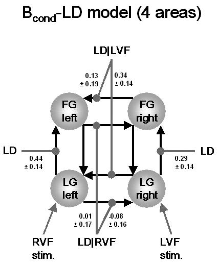
This figure shows the maximum a posteriori (MAP) estimates of the parameters (± square root of the posterior variances; units: 1/s=Hz) for the B_cond-LD model which, for the particular subject studied, proved to be the best of all 16 models tested. For clarity, only the parameters of interest, i.e. the modulatory parameters of inter- and intra-hemispheric connections, are shown and the bilateral visual field input has been omitted.

Since the difference between the best and the second-best model was not huge (see above), we also investigated the parameter estimates for the LD-B_cond model. In this model, task demands alone, independent of visual field, determined the strength of callosal connections. It was pleasing to find that this model gave compatible results in terms of the asymmetrical modulation of callosal connections. Here, there was a 95.6% confidence that modulation of the right LG→left LG connection by LD (0.43 ± 0.15 Hz) was larger than the equivalent modulation of the left LG→right LG connection by LD (0.03 ± 0.16 Hz). As with the B_cond-LD model, we were considerably less certain (67.7%) about this asymmetry for the callosal connections at the level of FG (0.31 ± 0.18 Hz vs. 0.19 ± 0.17 Hz).

Finally, we extended the B_cond-LD model to include left and right MOG. Fitting this six-area model to the data gave estimates which were only marginally different for the modulatory parameters of LG and FG connections discussed above (see Figure 7). In contrast, the MAP estimates for modulation of the callosal connections between left and right MOG were very close to zero (modulation of the right MOG→left MOG connection by LD|LVF: 0.01 ± 0.02 Hz; modulation of the left MOG→right MOG connection by LD|RVF: −0.01 ± 0.02 Hz). Given these very small effects, the contrast between these estimates unsurprisingly indicated that there was support for the presence of an asymmetry with regard to contextual modulation of callosal connections between left and right MOG: the probability p(c^Tη_θ|y > 0) = 54.2% was very close to the 50% margin, indicating that it is equally likely that c^Tη_θ|y is smaller or larger than zero.

Figure 7.

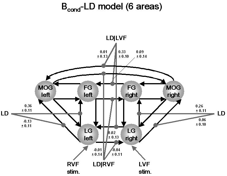
Parameter estimates for an extended version of the B_cond-LD model that includes the MOG in both hemispheres (see Fig. 5 for details). The estimates for callosal connections at the level of LG and FG were very similar to those from the four-area model (Fig. 5). In contrast to LG, there was no evidence for contextual modulation of callosal connections between right and left MOG.

Discussion

In this article we have summarized the theoretical foundations of DCM and BMS and have provided an example of the practical application of these techniques, using data from a single subject in the study by Stephan et al.³². DCM enables the investigation of how neural systems (composed of large neural populations like cortical areas) that have relatively high connectional complexity, e.g. multiple reciprocal connections and loops^11,23, operate. Together with BMS, DCM is a powerful tool to clarify which of multiple experimental manipulations (e.g. stimulus type, induction of cognitive set, learning processes etc.) have a significant impact on the dynamics of the network under investigation. By representing experimental factors as external inputs in the model, modeled effects can be interpreted fairly directly in neurobiological terms: any given DCM specifies precisely where inputs enter and whether they are driving (i.e. exert their effects through direct synaptic responses in the target area) or modulatory (i.e. exert their effects through changing synaptic responses in the target area to inputs from another area). This distinction, made at the level of neural populations, has a nice correspondence to empirical observations that single neurons can either have driving or modulatory effects on other neurons²³.

There are several ways in which DCM and DWI techniques can profit from each other. We have given a simple example in this paper of how models of effective connectivity like DCM are important for our understanding of processes in neural systems, even if their anatomical connectivity is well-understood. On the other hand, there are obviously many systems whose connectivity is less well-known than that of the corpus callosum and visual areas. In this case the specification of DCMs could be greatly facilitated by precise anatomical data on human brain connectivity obtained by DWI. Another potential opportunity is to use the likelihood of the existence of particular connections (as obtained from probabilistic tractography methods^7,8) as priors on connection strengths in Bayesian models like DCM.

In our empirical example, we demonstrated two things: in the particular individual studied, there is good evidence that (i) the measured data are best explained by a model in which inter-hemispheric interactions depend on task demands, but conditional on the visual field of stimulus presentation , and that (ii) there is a hemispheric asymmetry in context-dependent transcallosal interactions. Importantly, this asymmetry was not equally pronounced for all visual areas studied. It was particularly strong for the callosal connections between left and right LG: performance of the letter decision task specifically enhanced the strength of the influence of the right on the left LG, but only if the stimulus was presented in the left visual field and thus the information was initially only available in the right hemisphere. The reversed conditional effect, i.e. modulation of left LG→right LG by LD|RVF, was much weaker (and actually slightly negative, see Figures 5, 7). This result means that for the particular paradigm used enhancement of callosal connections was only necessary if stimulus information was initially represented in the “suboptimal”, i.e. right, hemisphere. Interestingly, in the subject analyzed, this asymmetry was less pronounced at the level of the FG and virtually absent at the level of the MOG.

These results complement very nicely our previous results on local activations elicited by this paradigm³². While we had previously established that, using identical stimuli in all conditions, a change in task demands was sufficient to determine the lateralization of brain activity, our previous analyses were not suited to clarify the principles according to which the two hemispheres functionally interacted. In other words, despite empirical data on context-dependent activations of visual areas and good knowledge about the general anatomical connectivity between these areas, we could not infer the mechanism by which transcallosal interactions contributed to the observed activations. In this paper, we have shown how this can be achieved by comparing different models, which are fitted to the empirical data, and then making statistical inferences about the parameters of the optimal model. It should be emphasized, however, that in this paper we have applied DCM to data from a single subject only, and it remains to be seen whether or not the principles of inter-hemispheric interactions found for the particular individual studied here generalize to the population. To clarify this question, we are currently analyzing the data from all subjects of the study by Stephan et al.³² following the strategy outlined in this article.

Group studies with DCM and BMS require somewhat different statistical procedures from those used in this paper. For example, when trying to find the optimal model for a group of individuals by BMS, it is likely that the optimal model will vary, at least to some degree, across subjects. An overall decision for n subjects can be made by computing an average Bayes factor which corresponds to the n-th root of the product of the individual Bayes factors (note that multiplication is appropriate because model comparisons from different individuals are statistically independent). Moreover, in this paper, all inferences about coupling parameters were based on the magnitude of the effect of interest (i.e. the contrast of the appropriate MAP estimates) compared to the precision with which this estimate was obtained (i.e. the posterior variance). When dealing with a group of subjects, one may be interested in different types of inference. For example, one may want to establish that a certain effect, e.g. the modulation of a particular connection by some experimental condition, is consistently expressed across subjects. This second-level inference can take various forms. For example, one can apply a classical statistical test to the parameters of interest or one can use a Bayesian approach, either treating the individual effects as fixed and combining the posterior variances or treating the individual parameters as random effects, thus enabling inference beyond the particular group of subjects studied⁴². These topics will be the subject of forthcoming methodological papers on DCM.

It should be noted that the idea underlying dynamic causal models is not restricted to fMRI data. David & Friston⁴³ have recently developed a neural mass model that, when combined with an appropriate forward model and estimation scheme, can be used as a DCM to derive neural coupling parameters from empirically measured electroencephalographic (EEG) or magnetoencephalographic (MEG) data (see David et al.⁴⁴ for a first application). This model has a much more sophisticated neural state equation than Eq. 2 in this paper, distinguishing between different cortical layers and different neural populations with specific time constants and connectivity. Furthermore, Harrison et al.⁴⁵ have developed a mean field model for event-related potentials that uses stochastic differential equations for the description of neural processes involving different types of transmitter receptors. The next years will see a further refinement of dynamic causal models of this kind.

We conclude by emphasizing that one of the long-term goals of developments related to DCM is to obtain tools for clinical applications. Such tools are particularly important for the study of psychiatric diseases like schizophrenia whose phenotypes are often confusingly heterogeneous due to strong interactions between genotype and environmental influences. One aim is to determine disease-specific endophenotypes; these are biological markers at intermediate levels between genome and behavior, e.g. particular neurophysiological or neurochemical indices⁴⁶. For example, if the pathophysiological mechanism that underlies a specific disease is an abnormal functional coupling between two or more brain regions in a particular context, this would correspond to a disease-specific pattern of coupling parameters in an appropriate DCM. The challenge for the future will be to establish valid neural systems models which can be fitted to measured imaging data and that are sensitive enough that their connectivity parameters can be used reliably for the diagnostic classification of individual patients. Ideally, such models should be used in conjunction with “implicit” paradigms that are minimally dependent on patient compliance, e.g. mismatch negativity paradigms⁴⁷. Given established validity and sufficient sensitivity of such a model, one could use it by analogy to a biochemical laboratory test, i.e. to compare a particular model parameter (or combinations thereof) against reference distributions in order to obtain diagnostic classifications. If the model is sophisticated enough to distinguish between different transmitter receptors, it might also be possible to obtain predictions for the optimal pharmacological treatment of individual patients. DCM, as described in this paper, provides a generic framework and starting point for this long-term endeavor.

References

- 1.Friston KJ. Beyond phrenology: What can neuroimaging tell us abut distributed circuitry? Ann. Rev. Neurosci. 2002;25:221–250. doi: 10.1146/annurev.neuro.25.112701.142846. [DOI] [PubMed] [Google Scholar]
- 2.Marshall JC, Fink GR. Cerebral localization, then and now. Neuroimage. 2003;20(Suppl. 1):S2–7. doi: 10.1016/j.neuroimage.2003.09.001. [DOI] [PubMed] [Google Scholar]
- 3.Köbbert C, Apps R, Bechmann I, et al. Current concepts in neuroanatomical tracing. Progr. Neurobiol. 2000;62:327–351. doi: 10.1016/s0301-0082(00)00019-8. [DOI] [PubMed] [Google Scholar]
- 4.Stephan KE, Kamper L, Bozkurt A, et al. Advanced database methodology for the Collation of Connectivity data on the Macaque brain (CoCoMac) Phil. Trans. R. Soc. Lond. B Biol. Sci. 2001;356:1159–1186. doi: 10.1098/rstb.2001.0908. [DOI] [PMC free article] [PubMed] [Google Scholar]
- 5.Bürgel U, Schormann T, Schleicher A, et al. Mapping of histologically identified long fiber tracts in human cerebral hemispheres to the MRI volume of a reference brain: position and spatial variability of the optic radiation. NeuroImage. 1999;10:489–499. doi: 10.1006/nimg.1999.0497. [DOI] [PubMed] [Google Scholar]
- 6.Galuske RA, Schlote W, Bratzke H, et al. Interhemispheric asymmetries of the modular structure in human temporal cortex. Science. 2000;289:1946–1949. doi: 10.1126/science.289.5486.1946. [DOI] [PubMed] [Google Scholar]
- 7.Behrens TEJ, Woolrich MW, Jenkinson M, Johansen-Berg H, Nunes RG, Clare S, Matthews PM, Brady JM, Smith SM. Characterization and propagation of uncertainty in diffusion-weighted MR imaging. Magn. Res. Med. 2003;50:1077–1088. doi: 10.1002/mrm.10609. [DOI] [PubMed] [Google Scholar]
- 8.Parker GJM, Haroon HA, Wheeler-Kingshott CAM. A framework for a streamline-based probabilistic index of connectivity (PICo) using a structural interpretation of MRI diffusion measurements. J. Magn. Res. Imag. 2003;18:242–254. doi: 10.1002/jmri.10350. [DOI] [PubMed] [Google Scholar]
- 9.Alexander DC, Barker GJ, Arridge SR. Detection and modeling of non-Gaussian apparent diffusion coefficient profiles in human brain data. Magn. Reson. Med. 2002;48:331–340. doi: 10.1002/mrm.10209. [DOI] [PubMed] [Google Scholar]
- 10.Strogatz SH. Exploring complex networks. Nature. 2001;410:268–276. doi: 10.1038/35065725. [DOI] [PubMed] [Google Scholar]
- 11.Friston KJ, Harrison L, Penny W. Dynamic causal modelling. Neuroimage. 2003;19:1273–1302. doi: 10.1016/s1053-8119(03)00202-7. [DOI] [PubMed] [Google Scholar]
- 12.Rockland KS, Pandya DN. Laminar origins and terminations of cortical connections of the occipital lobe in the rhesus monkey. Brain Res. 1979;179:3–20. doi: 10.1016/0006-8993(79)90485-2. [DOI] [PubMed] [Google Scholar]
- 13.Ringo JL, Doty RW, Demeter S, et al. Time is of the essence: a conjecture that hemispheric specialization arises from interhemispheric conduction delay. Cereb. Cortex. 1994;4:331–343. doi: 10.1093/cercor/4.4.331. [DOI] [PubMed] [Google Scholar]
- 14.Cavada C, Goldman-Rakic PS. Posterior parietal cortex in rhesus monkey: I. Parcellation of areas based on distinctive limbic and sensory corticocortical connections. J. Comp. Neurol. 1989;287:393–421. doi: 10.1002/cne.902870402. [DOI] [PubMed] [Google Scholar]
- 15.McGuire PK, Bates JF, Goldman-Rakic PS. Interhemispheric integration: I. Symmetry and convergence of the corticocortical connections of the left and the right principal sulcus (PS) and the left and the right supplementary motor area (SMA) in the rhesus monkey. Cereb. Cortex. 1991;1:390–407. doi: 10.1093/cercor/1.5.390. [DOI] [PubMed] [Google Scholar]
- 16.Funnell MG, Corballis PM, Gazzaniga MS. Insights into the functional specificity of the human corpus callosum. Brain. 2000;123:920–926. doi: 10.1093/brain/123.5.920. [DOI] [PubMed] [Google Scholar]
- 17.Westerhausen R, Kreuder F, Sequeira S, et al. Effects of handedness and gender on macro- and microstructure of the corpus callosum and its subregions: a combined high-resolution and diffusion-tensor MRI study. Cogn. Brain Res. 2004;21:418–426. doi: 10.1016/j.cogbrainres.2004.07.002. [DOI] [PubMed] [Google Scholar]
- 18.Hulshoff Pol HE, Schnack HG, Mandl RC, et al. Focal white matter density changes in schizophrenia: reduced inter-hemispheric connectivity. NeuroImage. 2003;21:27–35. doi: 10.1016/j.neuroimage.2003.09.026. [DOI] [PubMed] [Google Scholar]
- 19.Banich MT. The missing link: the role of interhemispheric interaction in attentional processing. Brain Cogn. 1998;36:128–157. doi: 10.1006/brcg.1997.0950. [DOI] [PubMed] [Google Scholar]
- 20.Bollen KA. Structural equations with latent variables. John Wiley; New York, NY: 1989. [Google Scholar]
- 21.Kennedy H, Dehay C, Bullier J. Organization of the callosal connections of visual areas V1 and V2 in the macaque monkey. J. Comp. Neurol. 1986;247:398–415. doi: 10.1002/cne.902470309. [DOI] [PubMed] [Google Scholar]
- 22.Segraves MA, Rosenquist AC. The afferent and efferent callosal connections of retinotopically defined areas in cat cortex. J. Neurosci. 1982;2:1090–1107. doi: 10.1523/JNEUROSCI.02-08-01090.1982. [DOI] [PMC free article] [PubMed] [Google Scholar]
- 23.Penny WD, Stephan KE, Mechelli A, et al. Comparing dynamic causal models. NeuroImage. 2004;22:1157–1172. doi: 10.1016/j.neuroimage.2004.03.026. [DOI] [PubMed] [Google Scholar]
- 24.Sherman SM, Guillery RW. On the actions that one nerve cell can have on another: distinguishing “drivers” from “modulators”. Proc. Natl. Acad. Sci. USA. 1998;95:7121–7126. doi: 10.1073/pnas.95.12.7121. [DOI] [PMC free article] [PubMed] [Google Scholar]
- 25.Buxton RB, Wong EC, Frank LR. Dynamics of blood flow and oxygenation changes during brain activation: the balloon model. Magn. Reson. Med. 1998;39:855–864. doi: 10.1002/mrm.1910390602. [DOI] [PubMed] [Google Scholar]
- 26.Friston KJ, Mechelli A, Turner R, et al. Nonlinear responses in fMRI: the Balloon model, Volterra kernels, and other hemodynamics. NeuroImage. 2000;12:466–477. doi: 10.1006/nimg.2000.0630. [DOI] [PubMed] [Google Scholar]
- 27.Friston KJ. Bayesian estimation of dynamical systems: an application to fMRI. NeuroImage. 2002;16:513–530. doi: 10.1006/nimg.2001.1044. [DOI] [PubMed] [Google Scholar]
- 28.Penny WD, Stephan KE, Mechelli A, et al. Modelling functional integration: a comparison of structural equation and dynamic causal models. NeuroImage. 2004;23:S264–274. doi: 10.1016/j.neuroimage.2004.07.041. [DOI] [PubMed] [Google Scholar]
- 29.Pitt MA, Myung IJ. When a good fit can be bad. Trends Cogn. Sci. 2002;6:421–425. doi: 10.1016/s1364-6613(02)01964-2. [DOI] [PubMed] [Google Scholar]
- 30.Stephan KE. On the role of general systems theory for functional neuroimaging. J. Anat. 2004;205:443–470. doi: 10.1111/j.0021-8782.2004.00359.x. [DOI] [PMC free article] [PubMed] [Google Scholar]
- 31.McIntosh AR, Grady CL, Ungerleider LG, et al. Network analysis of cortical visual pathways mapped with PET. J. Neurosci. 1994;14:655–666. doi: 10.1523/JNEUROSCI.14-02-00655.1994. [DOI] [PMC free article] [PubMed] [Google Scholar]
- 32.Stephan KE, Marshall JC, Friston KJ, et al. Lateralized cognitive processes and lateralized task control in the human brain. Science. 2003;301:384–386. doi: 10.1126/science.1086025. [DOI] [PubMed] [Google Scholar]
- 33.Jenner AR, Rosen GD, Galaburda AM. Neuronal asymmetries in primary visual cortex of dyslexic and nondyslexic brains. Ann. Neurol. 1999;46:189–196. doi: 10.1002/1531-8249(199908)46:2<189::aid-ana8>3.0.co;2-n. [DOI] [PubMed] [Google Scholar]
- 34.Amunts K, Schleicher A, Bürgel U, et al. Broca's region revisited: cytoarchitecture and intersubject variability. J. Comp. Neurol. 1999;412:319–341. doi: 10.1002/(sici)1096-9861(19990920)412:2<319::aid-cne10>3.0.co;2-7. [DOI] [PubMed] [Google Scholar]
- 35.Sergent J. Role of the input in visual hemispheric asymmetries. Psychol. Bull. 1983;93:481–512. [PubMed] [Google Scholar]
- 36.Levy J, Trevarthen C. Metacontrol of hemispheric function in human split-brain patients. J. Exp. Psychol. Hum. Percept. Perform. 1976;2:299–312. doi: 10.1037//0096-1523.2.3.299. [DOI] [PubMed] [Google Scholar]
- 37.Fink GR, Halligan PW, Marshall JC, et al. Where in the brain does visual attention select the forest and the trees? Nature. 1996;382:626–628. doi: 10.1038/382626a0. [DOI] [PubMed] [Google Scholar]
- 38.Abel PL, O'Brien BJ, Olavarria JF. Organization of callosal linkages in visual area V2 of Macaque monkey. J. Comp. Neurol. 2000;428:278–293. doi: 10.1002/1096-9861(20001211)428:2<278::aid-cne7>3.0.co;2-r. [DOI] [PubMed] [Google Scholar]
- 39.Kötter R, Stephan KE. Network participation indices: characterizing component roles for information processing in neural networks. Neural Netw. 2003;16:1261–1275. doi: 10.1016/j.neunet.2003.06.002. [DOI] [PubMed] [Google Scholar]
- 40.Schack B, Weiss S, Rappelsberger P. Cerebral information transfer during word processing: Where and when does it occur and how fast is it? Hum. Brain Mapp. 2003;19:18–36. doi: 10.1002/hbm.10104. [DOI] [PMC free article] [PubMed] [Google Scholar]
- 41.Nowicka A, Grabowska A, Fersten E. Interhemispheric transmission of information and functional asymmetry of the human brain. Neuropsychologia. 1996;34:147–151. doi: 10.1016/0028-3932(95)00064-x. [DOI] [PubMed] [Google Scholar]
- 42.Penny W, Holmes AP. Random-Effects Analysis. In: Frackowiack RSJ, et al., editors. Human Brain Function. Elsevier; San Diego, CA: 2004. pp. 843–850. [Google Scholar]
- 43.David O, Friston KJ. A neural mass model for MEG/EEG: coupling and neuronal dynamics. NeuroImage. 2003;20:1743–1755. doi: 10.1016/j.neuroimage.2003.07.015. [DOI] [PubMed] [Google Scholar]
- 44.David O, Harrison L, Kilner J, et al. Studying effective connectivity with a neural mass model of evoked MEG/EEG responses. In: Halgren E, Ahlfors S, Hämäläinen M, Cohen D, editors. Proceedings of the 14th international conference on biomagnetism (BIOMAG 2004); Boston, MA. 2004. pp. 135–138. [Google Scholar]
- 45.Harrison LM, David O, Friston KJ. Dynamic mean fields and ERP generation. Phil. Trans. R. Soc. Lond. B Biol. Sci. 2005 doi: 10.1098/rstb.2005.1648. in press. [DOI] [PMC free article] [PubMed] [Google Scholar]
- 46.Gottesman II, Gould TD. The endophenotype concept in psychiatry: etymology and strategic intentions. Am. J. Psychiatry. 2003;160:636–645. doi: 10.1176/appi.ajp.160.4.636. [DOI] [PubMed] [Google Scholar]
- 47.Baldeweg T, Klugman A, Gruzelier J, et al. Mismatch negativity potentials and cognitive impairment in schizophrenia. Schizophr. Res. 2004;69:203–217. doi: 10.1016/j.schres.2003.09.009. [DOI] [PubMed] [Google Scholar]