

Abstract
Common situations that result in different perceptions of grouping and border ownership, such as shadows and occlusion, have distinct sign-of-contrast relationships at their edge-crossing junctions. Here we report a property of end stopping in V1 that distinguishes among different sign-of-contrast situations, thereby obviating the need for explicit junction detectors. We show that the inhibitory effect of the end zones in end-stopped cells is highly selective for the relative sign of contrast between the central activating stimulus and stimuli presented at the end zones. Conversely, the facilitatory effect of end zones in length-summing cells is not selective for the relative sign of contrast between the central activating stimulus and stimuli presented at the end zones. This finding indicates that end stopping belongs in the category of cortical computations that are selective for sign of contrast, such as direction selectivity and disparity selectivity, but length summation does not.
Vision is an active integrative process: information from one part of the scene can drive the interpretation of features in other parts1. The information in an image is concentrated at contours and terminations2. Line ends, corners and junctions are singularities that are crucial for form perception, object recognition, depth ordering and motion processing (refs. 1,3-7). The physiological correlates of the perceptual phenomena of terminator detection and contour completion must begin with the well-known single-cell physiological properties of end stopping and length summation. Selective responsiveness to terminators (by end-stopped cells) probably provides the initial step both in depth ordering of contours and surfaces, and in solving the aperture problem for stereo and motion8-10. Similarly, the physiological property of length summation must provide the initial step in the process of contour integration.
To identify correctly the end of a contour, the brain must ignore changes in contrast caused by nonuniform illumination and respond only to those changes caused by the ending of the contour. Contrast polarity can be used to differentiate between these situations. If a change in contrast is due to an alteration in illumination, such as a shadow, then contrast polarity will be preserved along the contour. Conversely, contrast polarity inversion along a contour usually signals the end of the contour. Many instances of surface stratification and border ownership, such as shadow, transparency, occlusion and neon color spreading, have different ordinal contrast configurations at T and X junctions (Fig. 1). A long-standing issue is how the visual cortex uses contrast information to distinguish among different ordinal relations within these junctional singularities. Are there explicit junction detectors in the visual cortex?
Figure 1.

Sign of contrast along contour discontinuities drives border ownership and surface stratification. (a) Stable transparency with a transparent square appearing to lie above the bar; the sign of contrast is preserved along the edges of the bar but reverses along the square. (b) Stable transparency with a transparent bar appearing to lie above the square; the sign of contrast is preserved along the edges of the square but reverses along the bar. (c) Bistable transparency or shadow; the sign of contrast is preserved along the length of the bar and along the orthogonal sides of the square. (d) The contrast of the bar with the background reverses sign along the length of the contour; the bar does not look like a single continuous object, but rather as three segmented pieces. Does sign-of-contrast order sufficiently predict the perception? (e) A counterexample of sufficiency: the contrast reverses along the length of the bar, but this time the configuration is consistent with the perception of an occluding bar. Although the sign of contrast along the orientation of the bar is not sufficient to differentiate the grouping uniquely, when this information is combined with the orthogonal-edge signs of contrast, the three conditions in c-e are distinguishable. Thus, determination of the contrast relationships along contours that make up junctions must be a necessary step towards the grouping solution. (f) The square appears over the bar and shows neon spreading of luminance into the bar; the contrast along the bar is preserved. (g) Reversal of luminance in f; the bar now appears on top and the contrast along the bar reverses with no neon spreading. (h) Classical version of a; unambiguous transparency configuration. (i) Classical version of c; ambiguous transparency configuration. (j) Classical version of d; unrealistic configuration. (k) Illusory border version of f analogously shows bleeding of the square onto the background in the same way that the square in f bleeds onto the bar. (l) Amodal completion version of g analogously shows no bleeding; in the same way that the bar in g occludes the square, the background here appears to occlude an underlying dark square seen through four holes.
Although, perceptually, sign-of-contrast information at junctions is crucial, it is generally assumed that by the complex-cell stage of V1 information about sign of contrast has been pooled11 and is therefore not available for computations involving complex cells. Because both end stopping and length summation are observed in complex cells12-14, this notion presents a paradox, unless we assume that these computations occur at the antecedent to the simple-cell stage. Here we show that the well-known phenomenon of end stopping shows selectivity for sign of contrast, which would endow end-stopped cells with the ability to distinguish between contrast-conserving and contrast-reversing junctions and could therefore provide information essential for grouping in depth and border ownership.
RESULTS
End-zone interactions with moving bars
We recorded from 75 orientation-selective complex cells in V1 of two alert fixating macaque monkeys. On the basis of the length-summation properties of responses to single-contrast moving bars (Fig. 2a), cells were selected that were either end stopped or length summing. Cells were classified as being end stopped or length summing depending on whether their responses to the two longest bars were smaller than the optimal response: cells classified as length summing showed increasing responses with increasing stimulus length, so that the response was maximal to the longest bars; cells that were classified as end stopped showed an optimal response at a length shorter than the maximum. The sign-of-contrast selectivity of end stopping and length summation were assessed in each cell studied (Fig. 2) by using optimally oriented moving bars with independent center and wing segments (Fig. 2b).
Figure 2.
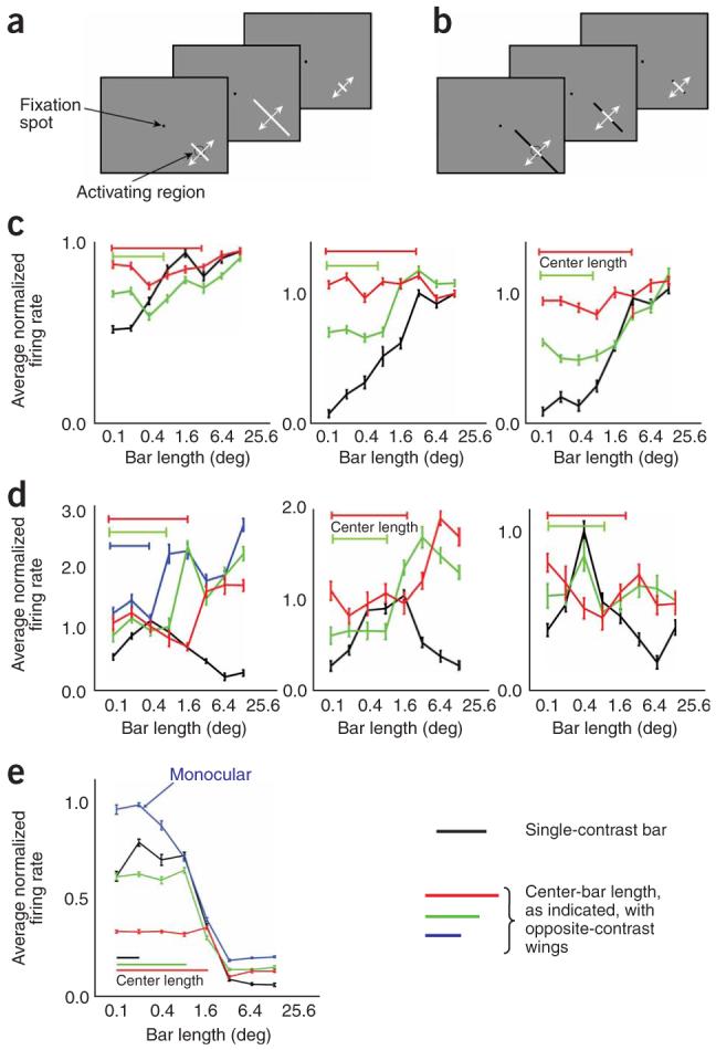
Sign-of-contrast selectivity of end stopping and length summation. (a) Stimulus configuration for classifying cells as length summing or end stopped. The stimulus was a plain black or white moving bar. (b) Stimulus configuration for determining sign-of-contrast selectivity of end-zone effects. The stimulus was a black or white moving bar with opposite-contrast wings. (c) Sign-of-contrast selectivity of length summation. Black curves indicate average normalized responses to a single-contrast bar moving back and forth across the receptive field (as in a) as a function of bar length, averaged for plain black and plain white bars. Colored lines show responses to a center bar of fixed length, as indicated, with opposite-contrast bilateral wings as a function of wing length; responses are averaged for white-center/black-wings bars and their reverse. (d) Sign-of-contrast selectivity of end stopping. Conventions as in c. (e) Interocular transfer properties of end-stopping interactions for a typical end-stopped cell. Blue trace shows the average of the monocular length-summation curves for the two eyes; other traces show responses to a central monocular bar, of the indicated length, as a function of wing length presented monocularly to the opposite eye, averaged over both eye combinations.
The sign-of-contrast selectivity of length tuning for three typical length-summing cells and three typical end-stopped cells is shown in Figure 2c,d, respectively. For each cell, the average length tuning for plain black or plain white bars (averaged together) is shown by the black lines; the colored lines show the length tuning of the same cells to bilateral wings of opposite contrast from a central bar of fixed length (as indicated), averaged over both contrast combinations. Population results for 75 cells are shown in Figure 3. All of the length-summing cells gave larger responses to bars that were longer than the activating region of the receptive field, irrespective of whether the wings were the same contrast as or the opposite contrast to the central bar. All of the end-stopped cells gave smaller responses to bars that were longer than the activating region of the receptive field, but only when the wings of the bar were the same contrast as the center of the bar; when the wings were of opposite contrast, they either enhanced the response or did not affect it. These results indicate that length summation is not selective for the sign of contrast between the activating region and the end zone, but end stopping is.
Figure 3.

Population results for the end-zone properties of end-stopped and length-summing cells. End-stopped cells (left) show suppressive interactions for same-contrast end-zone stimulation and facilitatory effects for opposite-contrast end-zone stimulation. These properties are distinct from those of length-summing cells (right), which show facilitatory effects for both same- and opposite-contrast end-zone stimulation.
The fact that end-stopping interactions invert for opposite-contrast stimulus pairs suggests that it arises early in the visual pathway, because only in center-surround cells (present in the retina, lateral geniculate nucleus and layer 4C of V1) or in simple cells are responses routinely selective for sign of contrast at any point in the receptive field. Complex cells, which are usually considered to represent the next stage after simple cells, respond similarly to light and dark stimuli in any part of the receptive field11. Therefore, because monocularity is also characteristic of early stages in the visual system, we investigated whether end-stopping interactions show interocular transfer. We found, however, that end-stopping interactions showed interocular transfer, with equally strong suppressive interactions from wings from either eye, when only one eye was stimulated in the center of the receptive field (Fig. 2e). A study in anesthetized cat also found that end-stopping interactions show interocular transfer15. We measured the magnitude of end stopping within and across eyes in 27 end-stopped cells. The average magnitude of the end-stopping index in the dichoptic condition was on average 80% of the monocular magnitude.
Reverse correlation mapping of end- and side-zone interactions
To explore the time course, spatial organization and spatial precision of end-stopping and length-summing influences, we used a sparse-noise technique in which four optimally oriented short bars (two white and two black bars) were presented in each frame at random positions centered around the activating region at a rate of 75 Hz (Fig. 4).
Figure 4.
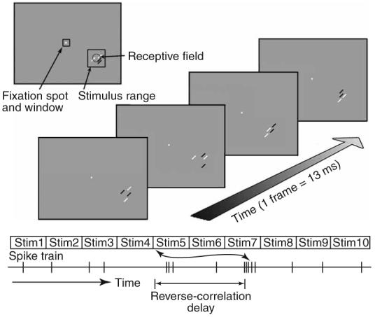
Stimulus configuration for sparse-noise reverse-correlation mapping of end-stopped and length-summing effects. In each frame, two white bars and two black bars were presented at random locations within a square stimulus range larger than the receptive field. The luminance of the bars was gamma-corrected; thus, the overlap of a back and a white bar canceled to background gray, and that of two black or two white bars resulted in a linear summation of whiter or darker luminance. For opposite-contrast interactions, spikes were reverse-correlated with all possible permutations of one black and one white bar and the resultant maps were averaged together. For the same-contrast maps, the same was done with all possible permutations of one white (or black) bar and the other white (or black) bar.
For sparse-noise reverse-correlation mapping, spikes were correlated with the difference in position of two of the bars in a preceding frame (probe-bar position minus reference-bar position) and normalized for the effect of each bar alone on the response of the cell (the first-order statistics). Unlike first-order (receptive field) maps, which show spike activity as a function of stimulus position, second-order maps show the average facilitatory or suppressive effect of one bar on the response of another, as a function of their relative position, irrespective of the absolute position of the two bars within the stimulus range. Because for any pair of bars in a frame each bar can be considered as the reference, there is a central symmetry to the maps. For example, the center of the map corresponds to occasions when the two bars were presented at the same location, and the top right of the map corresponds to occasions when either one of the bars was above and to the right of the other. Because the stimulus contained two white and two black bars in each frame, we had four potential same-contrast two-bar interactions (two white-white and two black-black interactions) and eight opposite-contrast two-bar interactions. We averaged the opposite-contrast interactions together, as well as the same-contrast interactions together.
Figure 5 shows the paired-bar interactions for three typical end-stopped cells. For each map a reference bar is drawn to scale at the center of the map; average facilitatory (red) and suppressive (blue) influences are shown for probe bars of the same and opposite contrast as the reference bar, which were presented simultaneously at various positions relative to each reference bar. Interaction maps are shown at two different delays because previous results from our laboratory have shown that end-stopping interactions develop more slowly than the excitatory response from the center of the receptive field8,10. At short reverse-correlation delays of 65 ms (corresponding to the average time to peak response to a bar presented at the center of the receptive field), the same-contrast maps show suppressive side-band interactions, as previously described16, and facilitatory end-zone interactions. At longer delays of 130 ms (corresponding to the average time to peak end-zone suppression), the side-band interactions become facilitatory and the end-zone interactions become suppressive. Previous studies have observed suppressive side-band interactions in complex cells and have suggested that they arise from the alternating on and off subfield organization of simple-cell inputs to complex cells16-18. Opposite-contrast interactions are the inverse: that is, facilitatory side-band interactions become suppressive over time, and weakly suppressive end-zone interactions become facilitatory over time.
Figure 5.
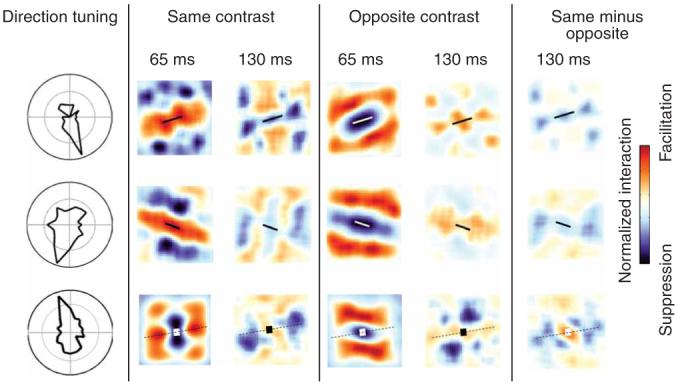
Paired-bar interaction maps for three end-stopped cells. Each row shows data for one cell. Direction tuning to moving bars is shown on the left; the optimal orientation is orthogonal to the preferred direction (dotted lines on the map). The interaction maps show the difference in response due to stimulus pairing as a function of distance between two bars when the two bars were of the same or opposite contrast, as indicated. Interactions are normalized to the maximum interaction for each cell. At reverse-correlation delays of 130 ms, the end zones are suppressive (blue) for same-contrast pairs and facilitatory (red) for opposite-contrast pairs. The sample bars at the center of each map show the scaled size and orientation of the bars used for stimuli. Dotted lines indicate the preferred orientation axis, on which end zones are centered.
Figure 6 shows the two-bar interactions for three typical lengthsumming cells. For each map, a reference bar is drawn to scale at the center of the map. As for the end-stopped cells, at short reverse-correlation delays the same-contrast maps show side-band suppression and end-zone facilitation, and the opposite-contrast maps show the inverse pattern. At longer delays, however, the end zones show only weak facilitatory interactions or no interactions for both same-contrast and opposite-contrast stimuli.
Figure 6.
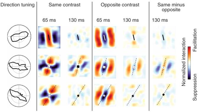
Paired-bar interaction maps for three length-summing cells. Note that at reverse-correlation delays of 130 ms, the end zones are facilitatory (or at least not suppressive) for both same-contrast pairs and opposite-contrast pairs. At a delay of 130 ms, side-band interactions of length-summing cells show more variability, particularly for opposite-contrast bars. Conventions as in Figure 5.
Figure 5 shows that the same-contrast endzone suppression in end-stopped cells appears after an initial same-contrast facilitatory interaction, whereas the reverse occurs for opposite-contrast end-zone suppression. In Figure 6, however, there is not a comparable inversion of the interaction pattern over time for length-summing cells.
Time course of end- and side-zone interactions
Figure 7 shows the time course of the population-average first-order responses from the center of the receptive field (Fig. 7a,b) compared with the average time courses of the second-order interactions in the end zones and the side zones for end-stopped and length-summing cells (Fig. 7c-f). Because the cells are complex, their responses to a black bar (Fig. 7a,b, black curve) are similar to their responses at the same position to a white bar (gray curve). The second-order responses are not invariant to sign of contrast: in end-stopped cells, the end-zone interactions for same-contrast bars show a delayed inhibitory phase (Fig. 7c, black curve), but the end-zone interactions for opposite-contrast bars (gray curves) are weakly facilitatory at that time. The opposite-contrast interactions in both end zones and side bands have a slower time course than do the same-contrast interactions. Length-summing cells, conversely, respond to end-zone and side-band stimuli in a simpler manner, both in timing and in the sign of activity: same-contrast bars show facilitatory interactions, whereas opposite-contrast bars show suppression. In addition, temporally the facilitatory and suppressive interactions in length-summing cells coincide with the first-order responses (compare Fig. 7b,d,f) and, unlike in end-stopped cells, do not show a delayed phase.
Figure 7.
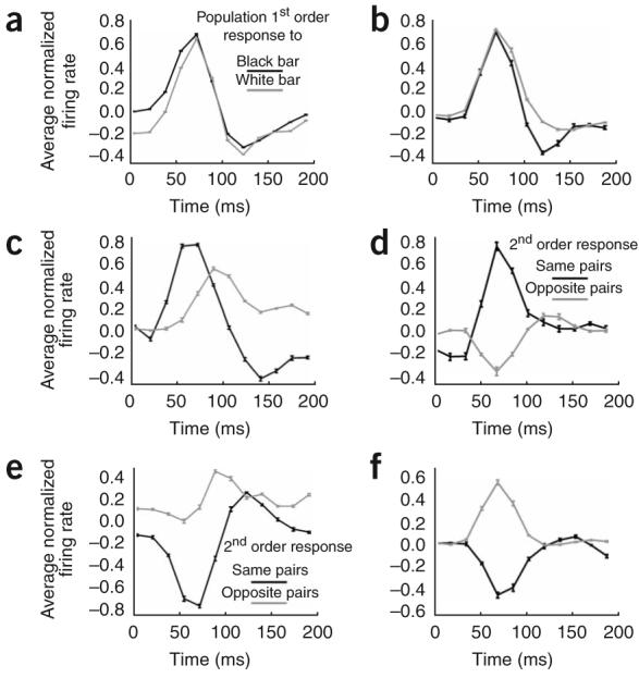
Time courses of first-order responses and second-order interactions in the end zones and the side bands. (a,c,e) End-stopped cells; (b,d,f) length-summing cells. (a,b) First-order responses to black or white bars presented at the center of the receptive field. Gray lines represent population-average responses to white stimuli; black lines represent responses to black stimuli. (c,d) End-zone interactions. (e,f) Side-band interactions. Black lines represent population-average second-order interactions between same-contrast stimulus pairs; gray lines represent interactions between opposite-contrast pairs.
DISCUSSION
We have shown that complex cells, which by definition show first-order response invariance for sign of contrast, are sensitive to sign of contrast in their second-order interactions along the orientation axis of their receptive field. Using both conventional moving bars and reverse-correlation mapping of responses to flashed bars, we found that end-stopped cells showed suppressive end-zone effects for bars of the same sign of contrast as the central activating bar, but showed no or a facilitatory effect for end-zone stimuli of opposite sign of contrast from the central bar. As previously reported, end-stopping interactions are delayed relative to the first-order response by about 70 ms (ref. 10).
It was initially suggested that only complex cells show end inhibition19, but subsequent studies found that both simple and complex cells can show end stopping20. It is not clear whether end stopping is generated by intracortical inhibitory circuits21-24 or subcortically from the inhibitory surrounds of lateral geniculate nucleus cells19,20,25,26. End stopping is resistant to the application of bicuculline, suggesting that it is not the result of intracortical inhibition, at least not γ-amino butyric acid (GABA)-mediated inhibition27. Intracellular recordings in anesthetized cat indicate, however, that end stopping involves both inhibitory inputs, which must be intracortical, and decreased excitatory currents, which could reflect either subcortical or cortical processes28.
Some researchers have argued that end stopping and side stopping are both manifestations of a nonspecific gain control or normalization mechanism29, whereas others argue that end and side stopping are qualitatively different from nonspecific surround suppression24,30,31. Lastly, it has been proposed that end stopping is an emergent property of the processing in the cortico-geniculate loop2,32,33. The strongest argument that end stopping is at least partly cortical in origin is that it is selective to orientation, being stronger when the elements in the end zone match the orientation of the excitatory stimulus in the center of the receptive field19,34,35. The fact that end stopping shows interocular transfer also supports a cortical origin (our results and ref. 24).
Previous studies in anesthetized cat found that end stopping is not phase sensitive24,36. This lack of phase sensitivity, as well as broader orientation- and spatial-frequency tuning, for end suppression was taken to indicate that end suppression arises largely from a nonselective suppressive network of cortical cells, similar to a gain control mechanism. This lack of selectivity implies that end stopping, at least in the anesthetized cat, should not be sensitive to the sign of contrast between a central and an end bar. These studies in cat did not measure the sign of contrast selectivity directly, however, and only end stopping arising from collinear simple cells would be expected to show phase selectivity. In addition, the design of the stimuli used to test phase sensitivity inserts a perpendicular reversing polarity edge that can interfere with the evaluation of phase sensitivity.
We found that end-zone suppression in complex cells was selective for sign of contrast, and this behavior was distinct from the sign-of-contrast invariancy of the first-order responses of complex cells. Thus, the phenomenon of end stopping cannot be a gain-control mechanism generated at the complex-cell stage, but must be inherited from earlier stages where sign-of-contrast selectivity is manifest. Because end-zone suppression shows interocular transfer, however, this potential stage is localized to the cortex after layer 4C.
Conversely, length-summing interactions were found to be unselective for sign of contrast, indicating a fundamental qualitative difference in mechanism between length summation and end stopping. The sign-of-contrast selectivity of end stopping could represent contrast-sensitive terminator detection, which has been postulated as necessary to explain the phenomena of transparency and neon color spreading36. The ability of end-stopped cells to discriminate the sign of contrast at terminators obviates the requirement for specific T-junction or X-junction detectors, because end-stopped cells could represent the contrast relationships along the edges of such junctions.
At least some aspects of figure-ground segregation are likely to be processed by low-level mechanisms, because manipulating stimuli to change perceived border ownership affects behaviors such as visual search37-39 and shape recognition40,41. In addition, the existence of ‘impossible’ figures, such as Penrose’s triangle, proves how important local cues can be: they can drive border ownership to generate perceptions of three-dimensional objects that violate higher-level object knowledge. One physiological manifestation of this process is the border-ownership property reported to be prevalent in area V2 (ref. 42): the short latency of border-ownership signals in V2 favors low-level mechanisms. Because this process is apparent in V2, the crucial input signals may arise in V1 and it is not unreasonable to suggest that the sign-of-contrast selectivity of end stopping that we observe in V1 cells may be a first step in surface stratification and border ownership.
METHODS
Electrophysiology
Single units were recorded in primary visual cortex of two alert fixating macaque monkeys. Two adult male macaque monkeys were prepared for chronic recording as described43,44. Monkeys fixated for a juice reward; data collected when the monkey’s eye position was more than 0.5° from fixation were discarded. Eye position was monitored by using a scleral search coil in a magnetic field45. All procedures were approved by the Harvard Medical Area Standing Committee on Animals.
Visual stimuli
Each cell was first tested for its orientation preference by using moving bars. Length tuning was then assessed at the preferred orientation by using single-contrast bars of varying length, which were moved back and forth across the center of the receptive field of each cell while the spiking activity of the cell was recorded. For each stimulus configuration, each possible length of the single bar or the wings was passed back and forth across the receptive field in random order for a sweep duration of 1 s; spikes were averaged for the whole sweep duration. For the moving-bar length-tuning protocol, we used a gray background so that the responses to white and black bars of optimal length on this background were matched. For the opposite-contrast wings model, the same background was used and the responses to black-center/white-wing stimuli were averaged with those to the white-center/black-wing stimuli. This averaging ensured that any lack of observed suppression to opposite-contrast wings was not due to a lack of response to one of the signs of contrast.
Data analysis
The degree of end stopping varies among cells. One way to classify a cell as end stopped is to set a threshold for the index of end stopping9. Here, however, we used a more concrete criterion to classify cells: end-stopped and end-summing cells were categorized by whether the length index of the cell was significantly negative or positive, respectively.
To make a quantitative comparison between cross-ocular and monocular end stopping, for every central bar length we compared the end-stopping index in both conditions. The end-stopping index was defined as follows:
where a is the spike rate for the central length present alone and b is the average plateau spike rate for the long bar.
For the histograms shown in Figure 3, we used the same formula with the exception that a stands for the response at the optimal length for that condition. The sign of the index is the same as the slope of length-tuning curve.
Reverse correlation mapping
For sparse-noise reverse-correlation mapping, two white (32.3 cd/m2) and two black (3.4 cd/m2) bar stimuli on a gray background (17.9 cd/m2) with the same optimum orientation were presented in each frame within a stimulus range that was centered on the receptive field of the cell. The frame rate was 75 Hz. When two bars overlapped, the super-position luminance was gamma-corrected to make the sum linear. For each map, between 50,000 and 100,000 spikes were collected over a duration of 35 min to 1 h. To generate first-order maps, the spike train (at 1-ms resolution) was reverse-correlated with black or white bar positions in the sequence of frames. Because there were two white bars and two black bars per frame, there were two first-order white bar maps and two first-order black bar maps; the two white maps were averaged together, as were the black maps.
For the second-order (interaction) maps, the spike train was reverse-correlated with the relative positions of pairs of bars; one bar was considered the reference and the other the probe. Spikes were reverse-correlated with the difference in position between the probe and the reference bar (probe position minus reference position). Because four bars were presented in each frame, there were four same-contrast maps (white1probe-white2ref and black1probe-black2ref plus the inverse) and eight opposite-contrast maps (white1probe-black1ref, white1probe-black2ref, white2probe-black1ref and white2probe-black2ref plus the inverse). For each cell, the same-contrast maps were similar and the opposite-contrast maps were similar, so we averaged all of the same-contrast maps and all of the opposite-contrast maps. To calculate only those spikes that were due to stimulus pairing (that is, the interactions), we had to eliminate the contribution of the first-order responses. For this, we subtracted maps in which there was a long (200-ms, noncausal) delay between the reference and the probe stimuli46. In the last column of Figures 6 and 7, we subtracted the opposite-contrast maps from the same-contrast maps, which is equivalent to calculating a second-order Wiener kernel47.
For the time courses of the first-order responses in Figure 7, we plotted the population-average response when the stimulus bars were presented within a 0.1 × 0.1° region centered on the receptive field of each cell. For the time courses of the second-order responses in Figure 7, we plotted the population-average interaction within a 0.1 × 0.1° interaction zone centered either on the end zone or the side zone.
ACKNOWLEDGMENTS
We thank D. Freeman for developing computer programs; T. Chuprina for technical assistance; R. Rajimehr for helpful input; C. Libedinsky for discussion; and D. Tsao for an analysis framework. This work was supported by a grant from the National Eye Institute (EY13135).
Footnotes
COMPETING INTERESTS STATEMENT
The authors declare that they have no competing financial interests.
References
- 1.Adelson EH. Lightness perception and lightness illusions. In: Gazzaniga M, editor. The New Cognitive Neurosciences. MIT Press; Cambridge, MA: 2000. pp. 339–351. [Google Scholar]
- 2.Attneave F. Some informational aspects of visual perception. Psychol. Rev. 1954;61:183–193. doi: 10.1037/h0054663. [DOI] [PubMed] [Google Scholar]
- 3.Beck J, Prazdny K, Ivry R. The perception of transparency with achromatic colors. Percept. Psychophys. 1984;35:407–422. doi: 10.3758/bf03203917. [DOI] [PubMed] [Google Scholar]
- 4.Watanabe T, Cavanagh P. The role of transparency in perceptual grouping and pattern recognition. Perception. 1992;21:133–139. doi: 10.1068/p210133. [DOI] [PubMed] [Google Scholar]
- 5.Watanabe T, Cavanagh P. Transparent surfaces defined by implicit X junctions. Vision Res. 1993;33:2339–2346. doi: 10.1016/0042-6989(93)90111-9. [DOI] [PubMed] [Google Scholar]
- 6.Watanabe T, Cavanagh P. Surface decomposition accompanying the perception of transparency. Spat. Vis. 1993;7:95–111. doi: 10.1163/156856893x00306. [DOI] [PubMed] [Google Scholar]
- 7.Grossberg S, Yazdanbakhsh A. Laminar cortical dynamics of 3D surface perception: stratification, transparency, and neon color spreading. Vision Res. 2005;45:1725–1743. doi: 10.1016/j.visres.2005.01.006. [DOI] [PubMed] [Google Scholar]
- 8.Howe PD, Livingstone MS. V1 partially solves the stereo aperture problem. Cereb. Cortex. doi: 10.1093/cercor/bhj077. published online 23 November 2005 (doi:10.1093/cercor/bhj077) [DOI] [PMC free article] [PubMed] [Google Scholar]
- 9.Pack CC, Born RT, Livingstone MS. Two-dimensional substructure of stereo and motion interactions in macaque visual cortex. Neuron. 2003;37:525–535. doi: 10.1016/s0896-6273(02)01187-x. [DOI] [PubMed] [Google Scholar]
- 10.Pack CC, et al. End-stopping and the aperture problem: two-dimensional motion signals in macaque V1. Neuron. 2003;39:671–680. doi: 10.1016/s0896-6273(03)00439-2. [DOI] [PubMed] [Google Scholar]
- 11.Hubel DH, Wiesel TN. Receptive fields, binocular interaction and functional architecture in the cat’s visual cortex. J. Physiol. (Lond.) 1962;160:106–154. doi: 10.1113/jphysiol.1962.sp006837. [DOI] [PMC free article] [PubMed] [Google Scholar]
- 12.Hammond P, Munden IM. Areal influences on complex cells in cat striate cortex: stimulus-specificity of width and length summation. Exp. Brain Res. 1990;80:135–147. doi: 10.1007/BF00228855. [DOI] [PubMed] [Google Scholar]
- 13.Gilbert CD. Laminar differences in receptive field properties of cells in cat primary visual cortex. J. Physiol. (Lond.) 1977;268:391–421. doi: 10.1113/jphysiol.1977.sp011863. [DOI] [PMC free article] [PubMed] [Google Scholar]
- 14.Grieve KL, Sillito AM. The length summation properties of layer VI cells in the visual cortex and hypercomplex cell end zone inhibition. Exp. Brain Res. 1991;84:319–325. doi: 10.1007/BF00231452. [DOI] [PubMed] [Google Scholar]
- 15.Ohzawa I, Freeman RD. The binocular organization of complex cells in the cat’s visual cortex. J. Neurophysiol. 1986;56:243–259. doi: 10.1152/jn.1986.56.1.243. [DOI] [PubMed] [Google Scholar]
- 16.Movshon JA, Thompson ID, Tolhurst DJ. Receptive field organization of complex cells in the cat’s striate cortex. J. Physiol. (Lond.) 1978;283:79–99. doi: 10.1113/jphysiol.1978.sp012489. [DOI] [PMC free article] [PubMed] [Google Scholar]
- 17.Livingstone M, Conway BR. Substructure of direction-selective receptive fields in macaque V1. J. Neurophysiol. 2003;89:2743–2759. doi: 10.1152/jn.00822.2002. [DOI] [PMC free article] [PubMed] [Google Scholar]
- 18.Szulborski RG, Palmer LA. The two-dimensional spatial structure of non-linear subunits in the receptive fields of complex cells. Vision Res. 1990;30:249–254. doi: 10.1016/0042-6989(90)90040-r. [DOI] [PubMed] [Google Scholar]
- 19.Hubel DH, Wiesel TN. Receptive fields and functional architecture in two nonstriate visual areas (18 and 19) of the cat. J. Neurophysiol. 1965;28:229–289. doi: 10.1152/jn.1965.28.2.229. [DOI] [PubMed] [Google Scholar]
- 20.Schiller PH, Finlay BL, Volman SF. Quantitative studies of single-cell properties in monkey striate cortex. I. Spatiotemporal organization of receptive fields. J. Neurophysiol. 1976;39:1288–1319. doi: 10.1152/jn.1976.39.6.1288. [DOI] [PubMed] [Google Scholar]
- 21.Bolz J, Gilbert CD. Generation of end-inhibition in the visual cortex via interlaminar connections. Nature. 1986;320:362–365. doi: 10.1038/320362a0. [DOI] [PubMed] [Google Scholar]
- 22.Dobbins A, Zucker SW, Cynader MS. Endstopped neurons in the visual cortex as a substrate for calculating curvature. Nature. 1987;329:438–441. doi: 10.1038/329438a0. [DOI] [PubMed] [Google Scholar]
- 23.Dobbins A, Zucker SW, Cynader MS. Endstopping and curvature. Vision Res. 1989;29:1371–1387. doi: 10.1016/0042-6989(89)90193-4. [DOI] [PubMed] [Google Scholar]
- 24.DeAngelis GC, Freeman RD, Ohzawa I. Length and width tuning of neurons in the cat’s primary visual cortex. J. Neurophysiol. 1994;71:347–374. doi: 10.1152/jn.1994.71.1.347. [DOI] [PubMed] [Google Scholar]
- 25.Cleland BG, Lee BB, Vidyasagar TR. Response of neurons in the cat’s lateral geniculate nucleus to moving bars of different length. J. Neurosci. 1983;3:108–116. doi: 10.1523/JNEUROSCI.03-01-00108.1983. [DOI] [PMC free article] [PubMed] [Google Scholar]
- 26.Rose D. Mechanisms underlying the receptive field properties of neurons in cat visual cortex. Vision Res. 1979;19:533–544. doi: 10.1016/0042-6989(79)90138-x. [DOI] [PubMed] [Google Scholar]
- 27.Sillito AM, Versiani V. The contribution of excitatory and inhibitory inputs to the length preference of hypercomplex cells in layers II and III of the cat’s striate cortex. J. Physiol. (Lond.) 1977;273:775–790. doi: 10.1113/jphysiol.1977.sp012123. [DOI] [PMC free article] [PubMed] [Google Scholar]
- 28.Anderson JS, et al. Membrane potential and conductance changes underlying length tuning of cells in cat primary visual cortex. J. Neurosci. 2001;21:2104–2112. doi: 10.1523/JNEUROSCI.21-06-02104.2001. [DOI] [PMC free article] [PubMed] [Google Scholar]
- 29.Heeger DJ. Normalization of cell responses in cat striate cortex. Vis. Neurosci. 1992;9:181–197. doi: 10.1017/s0952523800009640. [DOI] [PubMed] [Google Scholar]
- 30.Nelson JI, Frost BJ. Orientation-selective inhibition from beyond the classic visual receptive field. Brain Res. 1978;139:359–365. doi: 10.1016/0006-8993(78)90937-x. [DOI] [PubMed] [Google Scholar]
- 31.DeAngelis GC, et al. Organization of suppression in receptive fields of neurons in cat visual cortex. J. Neurophysiol. 1992;68:144–163. doi: 10.1152/jn.1992.68.1.144. [DOI] [PubMed] [Google Scholar]
- 32.Sillito AM, Cudeiro J, Murphy PC. Orientation sensitive elements in the corticofugal influence on centre-surround interactions in the dorsal lateral geniculate nucleus. Exp. Brain Res. 1993;93:6–16. doi: 10.1007/BF00227775. [DOI] [PubMed] [Google Scholar]
- 33.Murphy PC, Sillito AM. Corticofugal feedback influences the generation of length tuning in the visual pathway. Nature. 1987;329:727–729. doi: 10.1038/329727a0. [DOI] [PubMed] [Google Scholar]
- 34.Orban GA, Kato H, Bishop PO. Dimensions and properties of end-zone inhibitory areas in receptive fields of hypercomplex cells in cat striate cortex. J. Neurophysiol. 1979;42:833–849. doi: 10.1152/jn.1979.42.3.833. [DOI] [PubMed] [Google Scholar]
- 35.Cavanaugh JR, Bair W, Movshon JA. Selectivity and spatial distribution of signals from the receptive field surround in macaque V1 neurons. J. Neurophysiol. 2002;88:2547–2556. doi: 10.1152/jn.00693.2001. [DOI] [PubMed] [Google Scholar]
- 36.Tanaka K, et al. Receptive field properties of cells in area 19 of the cat. Exp. Brain Res. 1987;65:549–558. doi: 10.1007/BF00235978. [DOI] [PubMed] [Google Scholar]
- 37.Nakayama K, He Z, Shimojo S. Visual surface representation: a critical link between lower-level and higher-level vision. In: Kosslyn SM, Osherson D, editors. Visual Cognition: An Invitation to Cognitive Science. MIT Press; Cambridge, Massachu-setts: 1995. pp. 1–70. [Google Scholar]
- 38.He ZJ, Nakayama K. Surfaces versus features in visual search. Nature. 1992;359:231–233. doi: 10.1038/359231a0. [DOI] [PubMed] [Google Scholar]
- 39.Rensink RA, Enns JT. Early completion of occluded objects. Vision Res. 1998;38:2489–2505. doi: 10.1016/s0042-6989(98)00051-0. [DOI] [PubMed] [Google Scholar]
- 40.Nakayama K, Shimojo S, Silverman GH. Stereoscopic depth: its relation to image segmentation, grouping, and the recognition of occluded objects. Perception. 1989;18:55–68. doi: 10.1068/p180055. [DOI] [PubMed] [Google Scholar]
- 41.Driver J, Baylis GC. Edge-assignment and figure-ground segmentation in short-term visual matching. Cognit. Psychol. 1996;31:248–306. doi: 10.1006/cogp.1996.0018. [DOI] [PubMed] [Google Scholar]
- 42.Zhou H, Friedman HS, von der Heydt R. Coding of border ownership in monkey visual cortex. J. Neurosci. 2000;20:6594–6611. doi: 10.1523/JNEUROSCI.20-17-06594.2000. [DOI] [PMC free article] [PubMed] [Google Scholar]
- 43.Born RT, et al. Segregation of object and background motion in visual area MT: effects of microstimulation on eye movements. Neuron. 2000;26:725–734. doi: 10.1016/s0896-6273(00)81208-8. [DOI] [PubMed] [Google Scholar]
- 44.Livingstone MS. Mechanisms of direction selectivity in macaque V1. Neuron. 1998;20:509–526. doi: 10.1016/s0896-6273(00)80991-5. [DOI] [PubMed] [Google Scholar]
- 45.Judge SJ, Richmond BJ, Chu FC. Implantation of magnetic search coils for measurement of eye position: an improved method. Vision Res. 1980;20:535–538. doi: 10.1016/0042-6989(80)90128-5. [DOI] [PubMed] [Google Scholar]
- 46.Livingstone MS, Pack CC, Born RT. Two-dimensional substructure of MT receptive fields. Neuron. 2001;30:781–793. doi: 10.1016/s0896-6273(01)00313-0. [DOI] [PubMed] [Google Scholar]
- 47.Emerson RC, et al. Nonlinear directionally selective subunits in complex cells of cat striate cortex. J. Neurophysiol. 1987;58:33–65. doi: 10.1152/jn.1987.58.1.33. [DOI] [PubMed] [Google Scholar]