Abstract
The systematic development of reduced low-dimensional stochastic climate models from observations or comprehensive high-dimensional climate models is an important topic for atmospheric low-frequency variability, climate sensitivity, and improved extended range forecasting. Here techniques from applied mathematics are utilized to systematically derive normal forms for reduced stochastic climate models for low-frequency variables. The use of a few Empirical Orthogonal Functions (EOFs) (also known as Principal Component Analysis, Karhunen–Loéve and Proper Orthogonal Decomposition) depending on observational data to span the low-frequency subspace requires the assessment of dyad interactions besides the more familiar triads in the interaction between the low- and high-frequency subspaces of the dynamics. It is shown below that the dyad and multiplicative triad interactions combine with the climatological linear operator interactions to simultaneously produce both strong nonlinear dissipation and Correlated Additive and Multiplicative (CAM) stochastic noise. For a single low-frequency variable the dyad interactions and climatological linear operator alone produce a normal form with CAM noise from advection of the large scales by the small scales and simultaneously strong cubic damping. These normal forms should prove useful for developing systematic strategies for the estimation of stochastic models from climate data. As an illustrative example the one-dimensional normal form is applied below to low-frequency patterns such as the North Atlantic Oscillation (NAO) in a climate model. The results here also illustrate the short comings of a recent linear scalar CAM noise model proposed elsewhere for low-frequency variability.
Keywords: low-frequency teleconnection patterns, nonlinearity, correlated noise
There is recent interest in deriving reduced stochastic models for climate and extended-range weather prediction. An attractive property of atmospheric low-frequency variability is that it can be efficiently described by just a few large-scale teleconnection patterns. These patterns exert a huge impact on surface climate and seasonal predictability. Thus, such reduced stochastic models are an attractive alternative for extended range prediction and climate sensitivity studies because they are computationally much more efficient than state-of-the-art climate models and have been shown to have comparable prediction skill (1). Because such reduced models capture the essence of low-frequency processes they allow for a better understanding of the climate system. Thus, systematic strategies are essential in successfully developing reduced models. The recently developed stochastic mode reduction strategy provides a systematic procedure for the derivation of reduced stochastic models (2–6). In these studies the functional form of reduced models is systematically derived for geophysical flow models. In refs. 7 and 8 the procedure is refined to allow a seamless way of deriving stochastic low-order models from data of complex geophysical flow models. Of course, the predicted functional form (2–4, 6) can also be used for other procedures to infer stochastic models from data. Reduced models can also be used for climate sensitivity and climate change studies via the fluctuation dissipation theorem (FDT) (4, 9, 10). For example, there is a recent observational link (11) between the Greenland ice sheet collapse and changes in the primary low-frequency atmospheric teleconnection pattern in the Atlantic sector, the North Atlantic Oscillation (NAO).
The systematic stochastic mode reduction strategy (2–4, 6) predicts the functional form of the deterministic and stochastic terms. In particular, it predicts two types of noises. One is a simple additive noise, which stems from the nonlinear driving of the resolved scales by the unresolved scales, and the other is Correlated Additive and Multiplicative (CAM) noise. CAM noise has the following structural form:
where denotes a constant vector, a function, and a multivariate Wiener process. As 1 indicates, CAM noise acts both in a additive and multiplicative sense. As shown by refs. 3, 6–8, the multiplicative noise stems from the nonlinear advection of the resolved scales by the unresolved scales whereas the additive noise part stems from the linear operator. This linear operator is derived by linearizing the equations of motion around the climatological basic state.
In a recent study a linear scalar model with CAM noise is proposed for the description of climate variability (12). The proposed reduced model form from ref. 12 has several implications for scalar stochastic models of climate variables that are at odds with systematic procedures for the derivation of reduced stochastic models of climate variables (3, 6–8) and climate data (8, 13, 14). The linear CAM noise model of ref. 12 predicts a probability density function (PDF) whose tails decay according to a power law. This is certainly at odds with studies that examined a subspace spanned by the first few leading Empirical Orthogonal Functions (EOFs) from data generated by long integrations of general circulation models (8, 14) and reanalysis data (13, 15). These studies find only small, though significant, deviations from Gaussianity. These deviations occur most strongly in the form of excess skewness and to a much lesser extent in the form of excess kurtosis. Thus, there is not much empirical evidence for power-law decay of the tails of PDFs of the leading EOFs. Below we show that for a systematically derived scalar reduced stochastic climate model the PDF tails are dominated by a Gaussian decay due to cubic damping. However, this argument applies for low-frequency data (measured by the leading EOFs) and does not rule out the possible usefulness of the proposed form (12) for other climate variables at high frequencies in station data (16).
In the remainder of this study we will derive normal forms for nonlinear stochastic climate models, discuss the structural form of the PDF in the scalar case and utilize the normal forms for advanced parameter estimation of scalar climate variables for low-frequency teleconnection patterns such as the NAO.
Structural Implications of Energy Conservation for the Normal Form
The nature of the normal forms proposed here is tied to energy conservation of the nonlinear terms (3, 17, 18) as will be shown next.
The dynamical core of comprehensive large-scale models for the climate has the form
where F is a constant forcing, L a linear, and B a quadratically nonlinear operator, and u ∈ RM denotes the state vector with M ≫ 1. In Eq. 2 we assume that u denotes deviations from a climatological basic state and that basic state effects are already included in F and L (7). The quadratically nonlinear terms, B(u,u), alone arise from nonlinear advection, conserve energy, and, thus, satisfy the symmetry condition in Eq. 2.
The state vector u can be expanded into an orthonormal basis in the energy metric, . Then the conservation of energy constraint in Eq. 2 imposes the symmetries
for all indices l,j,k with 1 ≤ l,j,k ≤ M. In the special case where the orthonormal basis of variables ei are eigenfunctions of the Laplacian in spherical or periodic geometry, the eigenfunctions are exact solutions of the nonlinear operator and satisfy B(ei,ei) = 0; thus, the summands in 3 are non trivial only for i≠j≠k and are called triad interactions (2, 3, 17, 19); for theoretical purposes, this is the natural basis. However, in a general basis, e.g., of EOFs arising from low-frequency data analysis, B(ei,ei)≠0, and there are nontrivial dyad interactions which satisfy 3 for k = l,j = i
for 1 ≤ l ≤ M,i≠l,1 ≤ i ≤ M.
Now we partition the variable into low-frequency climate modes x ∈RN, N ≪ M, and high-frequency modes y ∈ RN′, N′ = M − N with x = (u1,…,uN) and y = (uN+1,…,uM). The goal of reduced climate models is to derive a stochastic model for the low-frequency variables, x, alone. The first step in deriving such a model is to rewrite the dynamical equation in 2 in terms of x and y; since the triad interactions have been discussed in detail elsewhere (2–4, 6, 19), we concentrate here on the additional phenomena associated with the interaction between the linear operator and the dyads
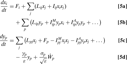 |
where the … denote triad interactions and interactions involving only unresolved modes and I denotes dyad interactions. The dyad interactions denoted by IA lead to uncorrelated additive noise and linear damping and the dyads IM together with the linear operator L produce CAM noise and deterministic quadratic nonlinear terms. In 5 we have utilized the important symmetries Iij = −Iji, IijM = −IjiM, and IijA = −IjiA, which are a consequence of energy conservation from 4 for dyads. Note, that ɛ is a parameter that denotes the timescale separation between the slow and fast variables and the stochastic mode reduction strategy is rigorously valid when ɛ → 0 (2–4, 6, 7).
Canonical Stochastic Model for a Scalar Low-Frequency Climate Variable
For a scalar reduced model, x ∈ R1, all low-frequency triad climate interactions vanish since all three variables are required to be distinct. We already know from the stochastic mode reduction procedure (2–4, 6, 7) that the IjpA terms produce additional damping and uncorrelated additive noise. For simplicity, and to concentrate on the new phenomena involving the interactions of multiplicative dyads with the linear operator, we do not discuss the effects arising from IjpA in detail in the following. Repeating the explicit mode elimination procedure for ɛ ≪ 1 (2–4, 6, 20) and coarse graining time as , which amounts to setting ɛ = 1, yields the normal form for scalar stochastic climate models in Stratonovich form
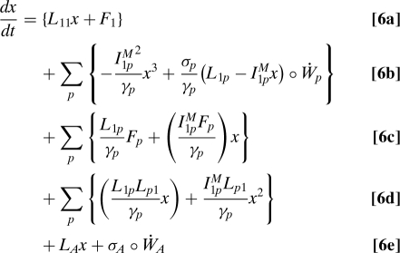 |
In 6 the summation over the index p denotes a summation over all unresolved variables. For ease of notation we rewrite 7 in Ito form as
 |
where , , , and . Here, LA is a linear damping coefficient and σA the variance of the white noise, and both terms arise from additive dyad or triad interactions. The white noises WA and Wp are mutually independent. We call the terms
CAM noise according to ref. 12. The key point is that when these terms are nonzero they simultaneously produce a cubic damping term in 7:
 |
Thus, CAM noise requires the presence of the cubic term because both are associated with the same dyad interactions and thus arise from the same physical process. This property has important implications for the form of the PDF and especially for the decay of its tails as we will show next.
The scalar stochastic climate model (7) has the associated Fokker–Planck equation
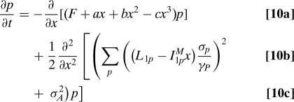 |
with p the probability density function.
The stationary distribution of (7) can be derived analytically by integrating the stationary Fokker–Planck equation Eq. 10 and is given by
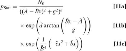 |
with , , , , , , and .
The factors in 11a and 11b are the type of PDF that arises from linear CAM noise alone (12) and that has unphysical power-law tails for any low-frequency pattern with significant variance; the above theory for dyad interactions automatically produces the factor in 11c with the Gaussian tail due to the cubic dissipation that ameliorates this unphysical effect.
The Normal Form in General Case of N Climate Variables
It is straightforward to generalize the normal form to N dimensions by using the above discussion together with that in refs. (2–4) including triad interactions. The result is given by
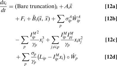 |
where the last line in 12 is a vector system of CAM noise. Again, it is clear from 12 that the existence of CAM noise is directly linked to the presence of the deterministic cubic terms. This property is linked to the energy conservation of the nonlinear operator. The cubic nonlinearity from the triad interactions (2, 3) represented by the second summand in 12c is also included since it is needed below.
Constraints on the N Dimensional Normal Forms
In practice (7, 14, 20) the original system has well-behaved PDFs for the low-frequency patterns with rapidly decaying tails; thus, the nonlinear operator in 12c should induce an effective damping.
This can be shown for the N dimensional case by multiplying 12 by xi, neglecting the noise terms and all other terms besides the cubic terms, and summing over i leading to the energy identity
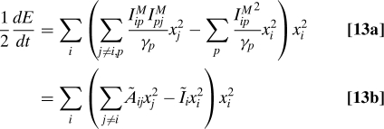 |
with , and . Eq. 13 can be written in matrix notation as
where 피 denotes the identity matrix. Eq. 14 is a quadratic form with . Stability of the original system now requires that . This is fulfilled if the quadratic form Q is negative-definite on the positive cone in ℝN. This is the equivalence in the N -dimensional case to the constraint of the coefficient of the cubic term c > 0 in one dimension from 9. This algebraic requirement constrains the normal form and shows that the cubic terms have to act effectively as damping and even allow the system to be linearly unstable.
Inverse Modeling and Parameter Estimation for Single-Variable Model
The functional form predicted by the mode elimination procedure developed above and in refs. 2, 3, 7, and 19, can be used to infer a stochastic climate model from time series, by estimating the model parameters from the data. For a 1-dimensional model with an stochastic differential equation (SDE) of the form (7) and associated Fokker–Planck equation of the form (10), there are 7 parameters to estimate as shown earlier. The drift and diffusion functions [A(x) and B(x)] in 10 have the form A(x) = F + ax + bx2 − cx3 and B(x) = B0 + B1x + B2x2. The parameters F,a,b,c,B0,B1,B2 can be inferred by using a parametric estimation procedure, under the constraints c ≥ 0, B0 ≥ 0, B2 ≥ 0. The last 2 constraints are necessary in order to have B(x) ≥ 0 for all x. In principle, one should also impose B12 ≤ 4B0B2 to guarantee B(x) ≥ 0. However, this makes the estimation more complicated; also, the estimated diffusions are all positive on the observed ranges of x. Therefore, we ignore the constraint B12 ≤ 4B0B2 here.
We use data from a quasi-geostrophic atmospheric circulation model with 3 vertical layers and horizontal triangular truncation at wavenumber 21 (T21) for the Northern Hemisphere with realistic climatological mean state, storm tracks, and low-frequency variability (8, 21) to estimate the parameters for a scalar reduced stochastic model. We utilize 6-h output data for a total of 50,000 days from the quasi-geostrophic model. The model is run under perpetual winter conditions. Hence, the parameters of the SDE in 7 are time-independent. From the data we take scalar time series for the leading Principal Components (PCs) of total energy EOFs (8) as well as a scalar time series resulting from the projection of the model stream function fields onto the observed NAO pattern at 500 hPa (8). The PCs and the NAO have only small deviations from Gaussianity in form of excess skewness (not shown; see refs. 8, 14, and 20). Each time series is rescaled by an overall constant factor so that it has unit variance; this facilitates parameter estimation and makes it easier to compare the relative size of the various terms in the normal form.
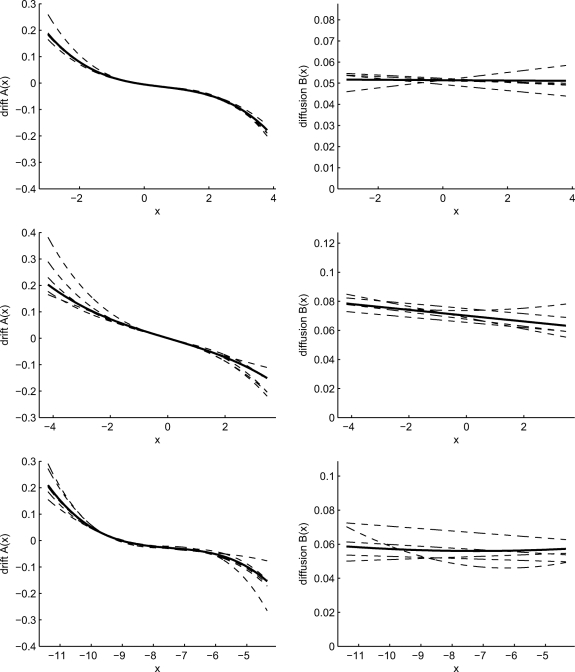
Given these (rescaled) scalar time series, we estimate the parameters by using a variant of the procedure developed in ref. 22. This estimation procedure is based on convex quadratic optimization and the use of leading eigenfunction–eigenvalue pairs of the Fokker–Planck operator. For each time series, the estimation is carried out 6 times: once using the entire time series and 5 times using different blocks of 10,000 days (nonoverlapping). For PCs 1 and 2, and the NAO, the resulting drift and diffusion functions are shown in Fig. 1. The functions are plotted over the entire range of x as observed in the time series. All of the three reduced stochastic models clearly have a cubic drift as predicted by the above theory with that for the NAO and PC1 more pronounced than that for PC2. Differences between the drift functions estimated from different blocks of the same time series are mainly visible in the tails of the probability distribution. The diffusion functions estimated from the time series are nearly constant, and PC2 has a weak linear slope. Quadratic terms in the diffusion functions for the PCs are either zero or so small that their contribution is not visible on the observed range of x. The diffusion functions estimated from the NAO time series show significant variance between the different blocks of data; nevertheless, most of the estimated functions are nearly constant.
Fig. 1.
Drifts and diffusions estimated from time series (rescaled to std = 1) for PC 1 (Top), PC 2 (Middle), and NAO (Bottom). Thick solid curves, results using all data; dashed curves, results from data divided into 5 nonoverlapping blocks.
All these results suggest that the additive noise terms from the climate base state dominate the diffusion process but the dyad interaction terms developed here make a significant nonlinear contribution to the drift for the low-frequency patterns in the present climate model.
Concluding Discussion
By using systematic principles from applied mathematics unique normal forms for reduced stochastic climate models for low-frequency teleconnection patterns have been developed here. Even for a scalar variable these normal forms predict a cubic nonlinear drift and a multiplicative correction to constant diffusion through CAM noise. The normal forms were applied in a parameter estimation strategy to fit the low-frequency patterns, such as the NAO, of a prototype climate model, and the confirmation of the predicted nonlinear cubic drift was evident in these results. Normal forms together with energy constraints were also developed here for reduced stochastic models in several dimensions. Important future directions should involve careful elucidation of the mathematical properties of the normal forms presented here, in conjunction with their implications through model estimation strategies for important issues in climate change response and prediction.
Acknowledgments.
A.J.M. is supported in part by National Science Foundation Grant DMS-0456713 and Office of Naval Research Grant N0014-05-1-1064. D.C. is supported by the Netherlands Organisation for Scientific Research through the research cluster Nonlinear Dynamics of Natural Systems.
Footnotes
The authors declare no conflict of interest.
References
- 1.Horenko I, Klein R, Dolaptchiev S, Schtte C. Automated generation of reduced stochastic weather models i: simultaneous dimension and model reduction for time series analysis. SIAM Mult Mod Sim. 2008;6:1125–1145. [Google Scholar]
- 2.Majda AJ, Timofeyev I, Vanden-Eijnden E. Models for stochastic climate prediction. Proc Natl Acad Sci USA. 1999;96:14687–14691. doi: 10.1073/pnas.96.26.14687. [DOI] [PMC free article] [PubMed] [Google Scholar]
- 3.Majda AJ, Timofeyev I, Vanden-Eijnden E. A mathematical framework for stochastic climate models. Commun Pure Appl Math. 2001;54:891–974. [Google Scholar]
- 4.Majda AJ, Abramov R, Grote M. Information Theory and Stochastics for Multiscale Nonlinear Systems. Providence, RI: American Mathematical Society; 2005. [Google Scholar]
- 5.Majda AJ, Franzke C, Fischer A, Crommelin DT. Distinct metastable atmospheric regimes despite nearly Gaussian statistics: A paradigm model. Proc Natl Acad Sci USA. 2006;103:8309–8314. doi: 10.1073/pnas.0602641103. [DOI] [PMC free article] [PubMed] [Google Scholar]
- 6.Majda AJ, Franzke C, Khouider B. An applied mathematics perspective on stochastic modelling for climate. Phil Trans R Soc A. 2008;366:2429–2455. doi: 10.1098/rsta.2008.0012. [DOI] [PubMed] [Google Scholar]
- 7.Franzke C, Majda AJ, Vanden-Eijnden E. Low-order stochastic mode reduction for a realistic barotropic model climate. J Atmos Sci. 2005;62:1722–1745. [Google Scholar]
- 8.Franzke C, Majda AJ. Low-order stochastic mode reduction for a prototype atmospheric GCM. J Atmos Sci. 2006;63:457–479. [Google Scholar]
- 9.Gritsun A, Branstator G. Climate response using a three-dimensional operator based on the fluctuation-dissipation theorem. J Atmos Sci. 2007;64:2558–2575. [Google Scholar]
- 10.Gritsun A, Branstator G, Majda AJ. Climate response of linear and quadratic functionals using the fluctuation-dissipation theorem. J Atmos Sci. 2008;65:2824–2841. [Google Scholar]
- 11.Holland DM, Thomas RH, De Young B, Ribergaard MH, Lyberth B. Acceleration of Jakobshavn Isbr triggered by warm subsurface ocean waters. Nature Geosci. 2008;1:659–664. [Google Scholar]
- 12.Sardeshmukh P, Sura P. Reconciling non-Gaussian climate statistics with linear dynamics. J Climate. 2009 10.1175/2008JCLI2358.1. [Google Scholar]
- 13.Sura P, Newman M, Penland C, Sardeshmukh P. Multiplicative noise and non-Gaussianity: A paradigm for atmospheric regimes? J Atmos Sci. 2005;62:1391–1409. [Google Scholar]
- 14.Berner J, Branstator G. Linear and nonlinear signatures in planetary wave dynamics of an AGCM: Probability density functions. J Atmos Sci. 2007;64:117–136. [Google Scholar]
- 15.Stephenson DB, Hannachi A, O'Neill A. On the existence of multiple climate regimes. Q J R Meteorol Soc. 2004;130:583–605. [Google Scholar]
- 16.Sura P, Sardeshmukh P. A global view of non-Gaussian SST variability. J Phys Oceonogr. 2008;38:639–647. [Google Scholar]
- 17.Salmon R. Lectures on Geophysical Fluid Dynamics. New York: Oxford Univ Press; 1998. [Google Scholar]
- 18.Timofeyev I. Systematic deviations from Gaussianity in models of quasigeostrophic turbulence. Phys Fluids. 2007 10.1063/1.2815728. [Google Scholar]
- 19.Majda AJ, Timofeyev I, Vanden-Eijnden E. A priori tests of a stochastic mode reduction strategy. Physica D. 2003;170:206–252. [Google Scholar]
- 20.Franzke C, Majda AJ, Branstator G. The origin of nonlinear signatures of planetary wave dynamics: Mean phase tendencies and contributions from non-Gaussianity. J Atmos Sci. 2007;64:3987–4003. [Google Scholar]
- 21.Marshall J, Molteni F. Toward a dynamical understanding of planetary-scale flow regimes. J Atmos Sci. 1993;50:1792–1818. [Google Scholar]
- 22.Crommelin DT, Vanden-Eijnden E. Reconstruction of diffusions using spectral data from timeseries. Commun Math Sci. 2006;4:651–668. [Google Scholar]


