Optimal Surface Segmentation in Volumetric Images—A Graph-Theoretic Approach

Abstract

Efficient segmentation of globally optimal surfaces representing object boundaries in volumetric data sets is important and challenging in many medical image analysis applications. We have developed an optimal surface detection method capable of simultaneously detecting multiple interacting surfaces, in which the optimality is controlled by the cost functions designed for individual surfaces and by several geometric constraints defining the surface smoothness and interrelations. The method solves the surface segmentation problem by transforming it into computing a minimum s-t cut in a derived arc-weighted directed graph. The proposed algorithm has a low-order polynomial time complexity and is computationally efficient. It has been extensively validated on more than 300 computer-synthetic volumetric images, 72 CT-scanned data sets of different-sized plexiglas tubes, and tens of medical images spanning various imaging modalities. In all cases, the approach yielded highly accurate results. Our approach can be readily extended to higher-dimensional image segmentation.

1 INTRODUCTION

The task of optimally identifying 3D surfaces representing object boundaries is important in segmentation and quantitative analysis of volumetric medical images. Many computer-based methods have been developed for optimal segmentation of 2D medical image data. Two-dimensional boundary-based segmentation utilizing graph-searching principles [1], [2], [3], [4], [5], [6], [7] has become one of the best understood and frequently utilized medical image segmentation tools. As a result, 3D medical images were usually analyzed as sequences of 2D image slices forming the 3D data. There are many essential problems associated with this approach—the most fundamental ones stem from the lack of contextual slice-to-slice information when analyzing sequences of adjacent 2D images. Obviously, performing the segmentation directly in the 3D space promises to produce more consistent segmentation results, yielding object surfaces instead of sets of individual contours. Previous attempts [8], [9], [10], [11], [12] on extending the graph-searching segmentation methods to higher dimensions either resulted in computationally intractable solutions or traded global optimality for efficiency, greatly limiting their utility.

In medical images, many surfaces that need to be identified appear in mutual interactions. These surfaces are “coupled” in a way that their topology and relative positions are usually known and the distances between them are within some specific range. Clearly, incorporating this surface-interrelation information into the segmentation will further improve its accuracy and robustness. Simultaneous segmentation of coupled surfaces in volumetric medical images is an underexplored topic, especially when more than two surfaces are involved.

Recently, we developed and validated a polynomial time method for d-D (d ≥ 3) optimal hypersurface detection with hard smoothness constraints, making globally optimal surface segmentation in volumetric images practical [13], [14]. By modeling the problem with a weighted geometric graph (a graph whose nodes and arcs are embedded in a geometric space), the method transforms the segmentation problem into computing a minimum s-t cut in a derived directed graph, which simplifies the problem and, consequently, solves it in a polynomial time. While the detection of a single optimal surface can be modeled by a 3D geometric graph [13], our novel method attempts to approach the simultaneous detection of k (k ≥ 2) interrelated surfaces by modeling the problem in a 4D geometric graph (or simply graph), where the fourth dimension consists of special arcs that control the interrelations between pairs of the sought surfaces. The apparently daunting combinatorial explosion in computation can be avoided by transforming the problems into computing minimum s-t cuts.

The main contribution of our work is that it extended the optimal graph-searching techniques to 3D and higher dimensions, while the backbone of our approach, graph cut, is radically different from traditional graph searching. This extension remains fully compatible with graph searching, i.e., in 2D, it produces identical result when the same objective function and hard constraints are employed. Consequently, many existing problems that were tackled using graph-searching in a slice-by-slice manner can be migrated to our new framework with little or no change to the underlying objective function formulation. The proposed method is limited to handling terrain-like (height-field) and cylindrical surfaces. This limitation seems severe at first sight. However, as we will demonstrate, the guarantee of global optimality and the freedom to design a problem-specific objective function allow the method to be applied to a variety of medical image segmentation problems. In the context, the method is referred to as a 3D approach regardless of the dimension of the graph being used, as opposed to the slice-by-slice (2D) approaches. Note that the preliminary results related to this research have been presented in a conference paper [15].

2 BACKGROUND AND RELATED WORK

2.1 Graph-Based Image Segmentation

Graph-based approaches have been playing an important role in image segmentation over the past several years. The general theme of these approaches is the formation of a weighted graph G = (V, E) with node set V and arc set E. The nodes v ∈ V correspond to image pixels (or voxels) and arcs 〈v_i, v_j 〉 ∈ E connect the nodes v_i,v_j according to some neighborhood system. Every arc 〈v_i,v_j〉 ∈E has a cost (or weight) representing some measure of preference that the corresponding pixels belong to the object of interest.

Depending on the specific application and the graph algorithm being used, the constructed graph can be directed or undirected. In a directed graph (or digraph), the arcs 〈v_i,v_j〉 and 〈v_j,v_i〉 (i ≠ j) are considered distinct and they may have different costs. If a directed arc 〈 v_i,v_j〉 exists, the node v_j is called a successor of v_i. A sequence of consecutive directed arcs 〈 v₀, v₁〉, 〈v₁, v₂〉,…,〈 v_k−1, v_k〉 form a directed path (or dipath) from v₀ to v_k.

Typical graph algorithms that were exploited for image segmentation include minimum spanning trees [16], [17], [18], [19], [20], shortest paths [7], [12], [21], [22], [23], [24], [25], [26], [27], and graph-cuts [28], [29], [30], [31], [32], [33], [34], [35], [36], [37]. Graph-cuts are relatively new and arguably the most powerful among all graph-based mechanisms for image segmentation. They provide a clear and flexible global optimization tool with considerably good computational efficiency.

The introduction of graph-cuts into medical image analysis happened only recently [14], [33], [38]. Classic optimal boundary-based techniques (e.g., dynamic programming, A* graph search, etc.) were used on 2D problems [27]. However, their 3D generalization, though highly desirable, has been unsuccessful for over a decade [8], [9], [10]. As a partial solution, region-based techniques such as region growing or watershed transforms were used. However, they suffer from an inherent problem of “leaking.” Advanced region growing approaches incorporated various knowledge-based or heuristic improvements (e.g., fuzzy connectedness) [21], [22]. The underlying shortest-path formulation of all these approaches has been revealed and generalized by the Image Foresting Transform (IFT) proposed by Falcão et al. [24]. Yet another class of powerful approaches to multi-dimensional image segmentation is based on level sets [39], [40].

2.2 Energy Minimization Using Graph-Cuts

The work most relevant to the method presented here is the energy minimization framework using minimum s-t cuts established by Boykov et al. [36], [41] and Kolmogorov et al. [42]. The cost function follows the “Gibbs” model [43]:

$$\epsilon \left(f\right)={\epsilon }_{\mathit{\text{data}}}\left(f\right)+{\epsilon }_{\mathit{\text{smooth}}}\left(f\right),$$

where f is a labeling of the image pixels. To minimize ε(f), a special class of arc-weighted directed graphs G_st =(V∪{s, t}, E) was employed. In addition to the nodes corresponding to image pixels (voxels), the node set of G_st contains two special terminal nodes, namely, the source s and the sink t. In image segmentation, the terminals typically correspond to the labels (e.g., object, background) that can be assigned to pixels. The arcs in G_st can be classified into two categories: n-links and t-links. n-links connect pairs of neighboring pixels whose costs are derived from the smoothness term ε_smooth(f). t-links connect pixels with terminals, whose costs are derived from the data term ε_data(f). An s-t cut (briefly, a cut) in G_st is a set of arcs whose removal partitions the nodes into two disjoint subsets S and T, such that s ∈ S and t ∈ T and no dipath can be established from s to t. The cost of a cut is the total cost of arcs in the cut. A minimum s-t cut is a cut whose cost is the minimum. The minimum s-t cut problem and its dual, the maximum flow problem, are classic combinatorial problems that can be solved by various polynomial-time algorithms [44], [45], [46].

It was proven that, if the arcs of G_st are properly constructed and their costs properly assigned, a minimum s-t cut in G_st can be used to exactly or approximately minimize ε(f) of certain forms in an efficient way. In turn, if an energy function is appropriately designed, a minimum s-t cut can segment an image into objects and background as desired. Several medical image segmentation techniques based on this framework were developed by Boykov and Jolly [33], [34] and Kim and Zabih [38]. Kim and Zabih’s method was designed specifically for contrast-enhanced MR images. Boykov and Kolmogorov’s algorithm [47] is flexible and shares some elegance with the level set methods. However, it needs the selection of object and background seed points, which is difficult to achieve for many applications. Besides, without taking advantage of the prior shape knowledge of the objects to be segmented, the results are topology-unconstrained and may be sensitive to initial seed point selections.

2.3 Segmentation of Coupled Surfaces

Due to the imperfections of medical imaging techniques, insufficient image-derived information may be available for defining an object boundary or surface. This insufficiency can be remedied by using clues from the other mutually related boundaries or surfaces. Cooptimization of multiple coupled surfaces thus frequently yields superior results compared to the traditional single-surface detection approaches.

Several methods for handling coupled surfaces have been proposed in recent years [48], [49], [50], [51]. None of them, however, guarantees a globally optimal solution. The method in [51] is essentially 2D and needs a precise manual initialization. The method in [49] is based on coupled parametric deformable models with self-intersection avoidance, which requires a complex objective function and is computationally expensive. The methods in [48], [50] utilize level-set formulations that can take advantage of efficient time-implicit numerical schemes [52]. They are, unfortunately, not topology-preserving [49], [53]. Further, the local boundary-based formulation in [48] can be trapped in a local minimum that is arbitrarily far away from the global optimum; while the introduction of a weighted balloon-force term may alleviate this difficulty [50], it exposes the model to a more hazardous “leaking” problem. Finally, the feasibility of extending these methods to handling more than two surfaces is unverified.

Active shape model (ASM) [54] and active appearance model (AAM) [55] implicitly take into account the geometric relations between surfaces due to the statistical shape constraints. Again, the frequently used iterative gradient descent methods may end at a local optimum [56]. Additionally, this model-based approach requires that point correspondence be established among instances of the training samples. Such 3D landmarking is difficult to achieve in general cases.

3 GRAPH CONSTRUCTION

A key innovation of our method is its nontrivial graph construction, aiming to transform the surface segmentation problem into computing a minimum closed set in a node-weighed digraph. A closed set C in a digraph is a subset of nodes such that all successors of any nodes in C are also contained in C. The cost of a closed set is the total cost of the nodes in the set. The minimum closed set problem is to search for a closed set with the minimum cost, which can be solved in polynomial time by computing a minimum s-t cut in a derived arc-weighted digraph [57].

3.1 Single Surface

A volumetric image can be viewed as a 3D matrix ℐ (x, y, z). Suppose a terrain-like surface in ℐ is oriented as shown in Fig. 1a. Let X, Y, and Z denote the image sizes in x, y, and z directions, respectively. The surface is defined by a function 𝒩 : (x, y) → 𝒩 (x, y), where x ∈ x = {0,…,X − 1}, y ∈ y = {0,…, Y − 1}, and 𝒩 (x, y) ∈ z = {0,…, Z − 1}. Thus, any surface in ℐ intersects with exactly one voxel of each column (of voxels) parallel to the z-axis, and it consists of exactly X × Y voxels. We refer to this model as a multicolumn model.

Fig. 1. The single-surface detection problem.

(a) The surface orientation. (b) Two adjacent columns of the constructed directed graph. Arcs shown in dashed lines are optional.

A surface is regarded feasible if it satisfies some application-specific smoothness constraint defined by two smoothness parameters, Δ_x and Δ_y. The smoothness constraint guarantees surface connectivity in 3D. More precisely, if ℐ (x, y, z) and ℐ (x + 1, y, z′) are two voxels on a feasible surface, then |z − z′| ≤ Δ_x. Likewise, if ℐ (x, y, z) and ℐ (x, y + 1, z′) are two voxels on a feasible surface, then |z − z′| ≤ Δ_y. If Δ_x (Δ_y) is small, any feasible surface is stiff along the x (y) direction, and the stiffness decreases with larger Δ_x (Δ_y).

By defining a cost function, a cost value is computed for each voxel ℐ (x, y, z) of ℐ, denoted by c(x, y, z). Generally, c(x, y, z) is an arbitrary real value that is inversely related to the likelihood that the desired surface contains the voxel ℐ (x, y, z). The cost of a surface is the total cost of all voxels on the surface. An optimal surface is the surface with the minimum cost among all feasible surfaces definable in the 3D volume.

A node-weighted directed graph G = (V,E) is constructed according to ℐ as follows: Every node V(x, y, z) ∈ V represents one and only one voxel ℐ(x, y, z) ∈ ℐ, whose cost w(x, y, z) is assigned according to:

$$w\left(x,y,z\right)=\{\begin{array}{cc}c\left(x,y,z\right)\hfill & \text{if}z=0,\hfill \\ c\left(x,y,z\right)-c\left(x,y,z-1\right)\hfill & \text{otherwise}\text{.}\hfill \end{array}$$ (1)

A node V(x, y, z) is above (respectively, below) another node V(x′, y′, z′) if z > z′ (respectively, z < z′). For each (x, y) pair with x ∈ x and y ∈ y, the node subset {V(x, y, z)|z ∈ z} is called the (x, y)-column of G, denoted by Col(x, y). Two (x, y)-columns are adjacent if their (x, y) coordinates are neighbors under a given neighborhood system. For instance, under the 4-neighbor setting, the column Col(x, y) is adjacent to Col(x + 1, y), Col(x − 1, y), Col(x, y + 1), and Col(x, y − 1). In the rest of this paper, the 4-neighbor system is assumed. The arcs of G consist of two types, intracolumn arcs and intercolumn arcs, constructed as follows. The goal of our construction is to transform the segmentation problem into a minimum closed set problem (Section 4.1).

Intracolumn arcs E^a

Along each column Col(x, y), every node V(x, y, z) (z > 0) has a directed arc to the node V(x, y, z − 1), i.e.,

$$E^a=\left\{\langle V\left(\mathbf{x},\mathbf{y},z\right),V\left(\mathbf{x},\mathbf{y},z-1\right)\rangle |z>0\right\}.$$ (2)

Intercolumn arcs E^r

Consider any two adjacent columns, Col(x, y) and Col(x + 1, y). Along the x-direction and for any x ∈ x, a directed arc is constructed from each node V(x, y, z) ∈2 Col(x, y) to node V(x + 1, y, max(0, z − Δ_x)) ∈ Col(x + 1, y). Similarly, a directed arc is connected from V(x + 1, y, z) ∈ Col(x + 1, y) to V(x, y, max(0, z − Δ_x)) ∈ Col(x, y). The same construction is done for the y-direction. These arcs enforce the smoothness constraints. In summary:

$$E^r=\{\begin{array}{c}\{\langle V\left(x,\mathbf{y},z\right),V\left(x+1,\mathbf{y},\text{max}(0,z-{\mathrm{\Delta }}_x\right))\rangle \hfill \\ \hfill |x\in \left\{0,\dots ,X-2\right\},z\in \mathbf{z}\}\cup \hfill \\ \{\langle V\left(x,\mathbf{y},z\right),V\left(x-1,\mathbf{y},\text{max}(0,z-{\mathrm{\Delta }}_x\right))\rangle \hfill \\ \hfill |x\in \left\{1,\dots ,X-1\right\},z\in \mathbf{z}\}\cup \hfill \\ \{\langle V\left(\mathbf{x},y,z\right),V\left(\mathbf{y},y+1,\text{max}(0,z-{\mathrm{\Delta }}_y\right))\rangle \hfill \\ \hfill |y\in \left\{0,\dots ,Y-2\right\},z\in \mathbf{z}\}\cup \hfill \\ \{\langle V\left(\mathbf{x},y,z\right),V\left(\mathbf{y},y-1,\text{max}(0,z-{\mathrm{\Delta }}_y\right))\rangle \hfill \\ \hfill |y\in \left\{1,\dots ,Y-1\right\},z\in \mathbf{z}\}.\hfill \end{array}$$ (3)

Intuitively, the intercolumn arcs guarantee that, if voxel ℐ(x, y, z) is on a feasible surface 𝒩, then its neighboring voxels on 𝒩 along the x-direction, ℐ (x + 1, y, z′), and ℐ (x − 1, y, z″), must be no “lower” than voxel ℐ (x, y, max(0, z − Δ_x)) (i.e., z′, z″ ≥ max(0, z − Δ_x)). The same rule applies to the y-direction. The intercolumn arcs make the node set V(x, y, 0) strongly connected, meaning that, in V(x, y, 0), every node is reachable from every other node through some dipath. V(x, y, 0) also forms the “lowest” feasible surface that can be defined inG. Because of this, the node set V(x, y, 0)is given a special name called the base set, denoted by V^B.

Sometimes, the desired surface is required to be wraparound along the x (or y) direction. This is common when segmenting a cylindrical surface, which is first unfolded into a terrain-like surface using cylindrical coordinate transform [27] before applying our algorithm (Fig. 2). Then, the first and last rows along the unfolding plane should satisfy the smoothness constraints as well. In the x-wraparound case, each node V(0, y, z) (respectively, V(X − 1, y, z)) also connects to V(X − 1, y, max(0, z − Δ_x)) (respectively, V(0, y, max(0, z − Δ_x))). The same rule applies to the y-wraparound case.

Fig. 2. Image unfolding.

(a) A tubular object in a volumetric image. (b) “Unfolding” the tubular object in (a) to form a new 3D image. The boundary of the tubular object in the original image corresponds to a surface to be detected in the unfolded image.

3.2 Multiple Surfaces

For simultaneously segmenting k (k ≥ 2) distinct but interrelated surfaces, the optimality is not only determined by the inherent costs and smoothness properties of the individual surfaces, but also confined by their interrelations.

If surface interactions are not considered, the k surfaces 𝒩_i can be detected in k separate 3D graphs. $G_i=\left(V_i,E_i\right)=\left(V_i,E_i^a\cup E_i^r\right)\left(i=1,\dots ,k\right).$ Each G_i is constructed in the way presented above. The node costs are computed utilizing k cost functions (not necessarily distinct), each of which is designed for detecting one surface. Taking the surface interrelations into account, another set of arcs E^s is needed, forming a directed graph G(V,E) in 4D space with $V={\cup }_{i=1}^k{V}_i\text{and}E={\cup }_{i=1}^k{E}_i\cup E^s.$ The arcs in E^s are called intersurface arcs, which model the pairwise relations between surfaces. For each pair of the surfaces, our approach defines their relations using two parameters, δ^l ≥ 0 and δ^u ≥ 0, representing the surface separation constraint.

The construction of E^s for double-surfaces segmentation is detailed below by examples. The ideas can easily be generalized to handling more than two surfaces.

In many practical problems, the surfaces are expected not to intersect or overlap. For instance, the inner and outer tissue walls should be noncrossing, and the distance between them should be within some expected range in the medical images. Suppose that, for two surfaces 𝒩₁ and 𝒩₂ to be detected, the prior knowledge requires 𝒩₂ to be below 𝒩₁. Let the minimum distance between them be δ^l voxel units and the maximum distance be δ^u voxel units. Let the 3D graphs used for the search of 𝒩₁ and 𝒩₂ be G₁ and G₂, respectively, and let Col₁(x, y) and Col₂(x, y) denote two corresponding columns in G₁ and G₂.

For any node V₁(x, y, z) in Col₁(x, y) with z ≥ δ^u, a directed arc in E^s connecting V₁(x, y, z) to V₂(x, y, z − δ^u) is constructed. Also, for each node V₂(x, y, z) in Col₂(x, y) with z < Z − δ^l, a directed arc in E^s connecting V₂(x, y, z) to V₁(x, y, z + δ^l) is introduced. This construction is applied to every pair of corresponding columns of G₁ and G₂.

Because of the separation constraint (𝒩₂ is at least δ^l voxel units below 𝒩¹), any node V₁(x, y, z) with z < δ^l cannot be on surface 𝒩₁. Otherwise, no node in Col₂(x, y) could be on surface 𝒩₂. Likewise, any node V₂(x, y, z) with z ≥ Z − δ^l cannot belong to surface 𝒩₂. These nodes that are impossible to appear in any feasible solution for the problem are called deficient nodes. Hence, for each column Col₁(x, y) ∈ G₁, it is safe to remove all nodes V₁(x, y, z) with z < δ^l and their incident arcs in E₁. Similarly, for each column Col₂(x, y) ∈ G₂, we safely eliminate all nodes V₂(x, y, z) with z ≥ Z − δ^l and their incident arcs in E₂.

Due to the removal of deficient nodes, the base set of G₁ becomes V₁(x, y, δ^l). Correspondingly, the cost of each node V₁(x, y, δ^l) is modified as w₁(x, y, δ^l) = c₁(x, y, δ^l), where c₁(x, y, δ^l) is the original cost of voxel ℐ (x, y, δ^l) for surface 𝒩₁. The intercolumn arcs of G₁ are modified to make V₁(x, y, δ^l) strongly connected. The base set of G then becomes V^B = V₁(x, y, δ^l) ∪ V₂(x, y, 0). The directed arc 〈V₁(0, 0, δ^l); V₂(0, 0, 0)〉 is introduced to E^s to make V_B strongly connected.

In summary, the intersurface arc set E^s for modeling two noncrossing surfaces is constructed as:

$$E^s=\{\begin{array}{c}\left\{\langle V_1\left(\mathbf{x},\mathbf{y},z\right),V_2\left(\mathbf{x},\mathbf{y},z-{\delta }^u\right)\rangle |z\ge {\delta }^u\right\}\cup \hfill \\ \left\{\langle V_2\left(\mathbf{x},\mathbf{y},z\right),V_1\left(\mathbf{x},\mathbf{y},z+{\delta }^l\right)\rangle |z<Z-{\delta }^l\right\}\cup \hfill \\ \left\{\langle V_1\left(0,0,{\delta }^l\right),V_2\left(0,0,0\right)\rangle \right\}.\hfill \end{array}$$ (4)

In other situations, we may allow the two interacting surfaces to cross each other. This is encountered when tracking a moving surface over time. For these problems, instead of modeling the minimum and maximum distances between them, δ^l and δ^u specify the maximum distances that a surface can vary below and above the other surface, respectively. The intersurface arcs for this case consist of the following: 〈V₁(x, y, z), V₂(x, y, max(0, z − δ^l))〉 and 〈V₂(x, y, z), V₁(x, y, max(0, z − δ^u))〉 for all x ∈ x, y ∈ y, and z ∈ z. A summary of all cases is illustrated in Fig. 3.

Fig. 3. Summary of surface interrelation modeling.

𝒩₁ and 𝒩₂ are two desired surfaces. Col₁(x, y) and Col₂(x, y) are two corresponding columns in the constructed graphs. Arcs shown in dashed lines are optional. (a) The noncrossing case. (b) The case with crossing allowed.

4 SURFACE DETECTION ALGORITHM

The segmentation of multiple coupled surfaces is formulated as computing a minimum closed set in a 4D geometric graph constructed from ℐ. The time bound of our algorithm is independent of both the smoothness parameters (Δ_xi and Δ_yi, i = 1, …, k) and the surface separation parameters (δ^l _i,i+1 and δ^u _i,i+1, i = 1,…,k − 1). In general, we refer to the smoothness constraints and surface separation constraints altogether as geometric constraints.

Note that improper specifications of the geometric constraints may lead to an infeasible problem, i.e., the constraints are self-conflicting and, thus, no k surfaces satisfying all the constraints exist in ℐ. The feasibility of the problem is easy to determine. Hence, we assume that the problem is feasible.

4.1 The Minimum Closed Set

In Section 3, the construction of a node-weighted directed graph G = (V,E) from the volumetric data set ℐ (x, y, z) was described.

In the single-surface case, for any feasible surface 𝒩 in ℐ, the subset of nodes on or below 𝒩 in G, namely, C = {V(x, y, z)|z ≤ 𝒩(x, y)} forms a closed set in G. It can be observed that, if V(x, y, z) is in the closed set C, then all nodes below it on Col(x, y) are also in C. Moreover, due to the node cost assignments in (1), the costs of 𝒩 and C are equal. In fact, as proven in [13], any feasible 𝒩 in ℐ uniquely corresponds to a nonempty closed set C in G with the same cost. This is a key observation to transforming the optimal surface problem into seeking a minimum closed set in G.

For concurrent segmentation of k coupled surfaces, the graph G consists of k disjoint 3D subgraphs {G_i = (V_i, E_i)|i = 1,…,k}, each of which is dedicated to searching for one surface. The separation constraints between any two surfaces are enforced in G by arcs between the corresponding subgraphs. By a similar argument as in the single-surface case, the construction of G establishes the following lemmas:

• Lemma 1. Any k feasible surfaces in ℐ correspond to a nonempty closed set in G with the same total cost.

• Lemma 2. Any nonempty closed set in G defines k feasible surfaces in ℐ with the same total cost.

In general, we are able to prove the following lemma, showing that computing the optimal k surfaces in ℐ is equivalent to finding a minimum nonempty closed set C* in G.

• Lemma 3. A minimum nonempty closed set C* in G specifies the optimal k surfaces in ℐ.

Note that a closed set C in a graph can be empty (with a cost zero). If the minimum closed set C* in G is empty, C* gives little useful information for defining the optimal k surfaces in ℐ. Fortunately, our careful construction of G still enables us to overcome this difficulty. If the minimum closed set in G is empty, it implies that the cost of any nonempty closed set in G is nonnegative. Since the base set V^B of G is strongly connected and it forms the “lowest” k feasible surfaces, it is always contained in any nonempty closed set in G. Therefore, to guarantee that the minimum closed set in G has a negative cost (and, thus, is nonempty), the costs of any nodes in V^B are reassigned to an arbitrary negative value (e.g., −1). This operation translates the cost of any nonempty closed set in G by a negative constant and is called the translation operation. After translation, we can simply find a minimum closed set C* in G, and C* is the minimum nonempty closed set in G before the translation.

Since the base set V^B is always contained in any nonempty closed set in G, the directed arcs connecting nodes not in V^B to the nodes in V^B (shown as dashed lines in Fig. 1b and Fig. 3) are optional. This gives rise to a very interesting observation: The graph is actually getting smaller (i.e., with fewer arcs) as the geometric constraints are relaxed (i.e., Δ and/or δ become larger). This behavior is just the opposite of the traditional graph-search-based algorithms for the problem.

4.2 Computing Optimal k Surfaces

Based on Lemma 3, we need to compute a minimum-cost nonempty closed set C* in G, which is a well studied problem in graph theory. As in [13], [57], and [58], we compute C* in G by computing a minimum s-t cut in a related graph G_st.

Let V⁺ and V⁻ denote the sets of nodes in G with nonnegative and negative costs, respectively. Define a new directed graph G_st = (V ∪ {s, t}, E ∪ E_st). The node set of G_st is the node set V of G plus a source s and a sink t. The arc set of G_st is the arc set E of G plus a new arc set E_st. We assign an infinity cost to each arc in E. E_st consists of the following arcs: The source s is connected to each node v ∈ V⁻ by a directed arc of cost −w(v); every node v ∈ V⁺ is connected to the sink t by a directed arc of cost w(v). Let (S, T) denote a finite-cost s-t cut in G_st and c(S, T) denote the total cost of the cut. It was proved that

$$c\left(S,T\right)=-w\left(V^{-}\right)+{\displaystyle \sum _{v\in S-\left\{s\right\}}w\left(v\right)},$$

where w(V⁻) is fixed and is the cost sum of all nodes with negative costs in G. Since S − {s} is a closed set in G [57], [58], the cost of a cut (S, T) in G_st and the cost of the corresponding closed set in G differ by a constant. Hence, the source set S* − {s} of a minimum cut in G_st corresponds to a minimum closed set C* in G.

Because the graph G_st has 𝒪(kn) nodes and 𝒪 (kn) arcs, the minimum closed set C* in G can be computed in 𝒯(kn, kn) time, herein, 𝒯(kn, kn) is the time for finding a minimum s-t cut in an arc-weighted directed graph with 𝒪(kn) nodes and 𝒪(kn) arcs.

The optimal k surfaces correspond to the upper envelope of the minimum closed set C*. They can be recovered in the following way: For each i (i = 1,…,k), recall that the subgraph G_i is used to search for the target surface N_i. For every x ∈ x and y ∈ y, let V_i^B (x, y) be the subset of nodes in both C* and the (x, y)-column Col_i(x, y) of G_i, i.e., V_i^B (x, y) = C* ∩ Col_i(x, y). Denote by V_i(x, y, z*) the node in V_i^B (x, y) with the largest z-coordinate. Then, voxel ℐ(x, y, z*) is on the ith optimal surface $N_i^{*}.$ In this way, the minimum closed set C* of G uniquely defines the optimal k surfaces $\left\{N_1^{*},\dots ,N_k^{*}\right\}$in ℐ.

To sum up, we have the following theorem:

• Theorem 1. The optimal k surfaces in a 3D image ℐ (x, y, z) with n voxels can be computed in 𝒯 (kn, kn) time.

Finally, the outline of the algorithm is:

• Input: k, Δ_x, Δ_y, δ^l, δ^u, and the cost function(s).

• Construct the graph G_st (= (V ∪ {s, t}, E ∪ E_st)).

• Compute the minimum s-t cut (S*, T*) in G_st.

• Recover the k optimal surfaces from S* − {s}.

5 COST FUNCTIONS

Designing appropriate cost functions is of paramount importance for any graph-based segmentation method. In real-world problems, the cost function usually reflects either a region-based or edge-based property of the surface to be identified.

5.1 Edge-Based Cost Functions

A typical edge-based cost function aims to accurately position the boundary surface in the volumetric image. Such a cost function may, e.g., utilize a combination of the first and second derivatives of the image intensity function [59], and may consider the preferred direction of the identified surface.

Let the analyzed volumetric image be ℐ (x, y, z). Then, the cost c(x, y, z) assigned to the image voxel ℐ(x, y, z) can be constructed as:

$$c\left(x,y,z\right)=-e\left(x,y,z\right)·p\left(\varphi \left(x,y,z\right)\right)+q\left(x,y,z\right),$$ (5)

where e(x, y, z) is a raw edge response derived from the first and second derivatives of the image and ϕ(x, y, z) denotes the edge orientation at location (x, y, z) that is reflected in the cost function via an orientation penalty p(ϕ (x, y, z)). 0 < p < 1 when ϕ(x, y, z) falls outside of a specific range around the preferred edge orientation; otherwise, p = 1. A position penalty term q(x, y, z) > 0 may be incorporated so that a priori knowledge about expected border position can be modeled:

$$\begin{array}{c}e\left(x,y,z\right)=\left(1-\left|\omega \right|\right)·\left(ℐ*{ℳ}_{\text{first}\text{derivative}}\right)\left(x,y,z\right)\hfill \\ \dot{+}\omega ·\left(ℐ*{ℳ}_{\text{second}\text{derivative}}\right)\left(x,y,z\right).\end{array}$$ (6)

The +˙ operator stands for a pixel-wise summation, and * is a convolution operator. The weighting coefficient −1 ≤ ω ≤ 1 controls the relative strength of the first and second derivatives, allowing accurate edge positioning. The values of ω, p, and q may be determined from a desired boundary surface positioning information in a training set of images (Section 6.2).

5.2 Nonedge-Based Cost Functions

The object boundaries do not have to be defined by gradients. For example, a piecewise constant minimal variance criterion based on the Mumford-Shah functional [60] was proposed by Chan and Vese [61] to deal with such situations:

$$\begin{array}{cc}\epsilon \left(S,a_1,a_2\right)=\hfill & {\displaystyle {\int }_{\mathit{\text{inside(S)}}}{\left(ℐ\left(x,y,z\right)-a_1\right)}^{2}dxdydz}\hfill \\ \hfill & +{\displaystyle {\int }_{\mathit{\text{outside(S)}}}{\left(ℐ\left(x,y,z\right)-a_2\right)}^{2}dxdydz.}\hfill \end{array}$$ (7)

The two constants a₁ and a₂ are the mean intensities in the interior and exterior of the surface S, respectively. The energy ε(S, a₁, a₂) is minimized when S coincides with the object boundary and best separates the object and background with respect to their mean intensities.

The variance functional can be approximated using our per-voxel cost model and, in turn, can be minimized using our graph-based algorithm. Since the application of the Chan-Vese cost functional may not be immediately obvious, let us consider a single-surface segmentation example. Any feasible surface uniquely bipartitions the graph into two disjoint subgraphs. One subgraph consists of all nodes that are on or below the surface, and the other subgraph consists of all nodes that are above the surface. Without loss of generality, let a node on or below a feasible surface be considered as being inside the surface; otherwise, let it be outside the surface. Then, if a node V(x′, y′, z′) is on a feasible surface 𝒩, then the nodes V(x′, y′, z′) in Col(x′, y′) with z ≤ z′ are all inside 𝒩, while the nodes V(x′, y′, z′) with z > z′ are all outside 𝒩. Hence, the voxel cost c(x′, y′, z′) is assigned as the sum of the inside and outside variances computed in the column Col(x′, y′) as follows:

$$\begin{array}{cc}c\left(x^{\prime },y^{\prime },z^{\prime }\right)=\hfill & {\displaystyle \sum _{z\le z^{\prime }}{\left(ℐ\left(x^{\prime },y^{\prime },z\right)-a_1\right)}^2}\hfill \\ \hfill & +{\displaystyle \sum _{z>z^{\prime }}{\left(ℐ\left(x^{\prime },y^{\prime },z\right)-a_2\right)}^2.}\hfill \end{array}$$ (8)

Then, the total cost of 𝒩 will be equal to ε(𝒩, a₁; a₂) (discretized on the grid (x, y, z)). However, the constants a₁ and a₂ are not easily obtained since the surface is not well-defined before the global optimization is performed. Therefore, the knowledge of which part of the graph is inside and outside is unavailable. Fortunately, our graph construction guarantees that, if V(x′, y′, z′) is on 𝒩, then the nodes V(x, y, z₁) with z₁ ≡ {z|z ≤ max(0, z′ − |x − x′|Δ_x − |y − y′|Δ_y)} are in the closed set C corresponding to 𝒩. Accordingly, the nodes V(x, y, z₂) with z₂ ≡ {z|z′ + |x − x′|Δ_x + |y − y′|Δ_y < z < Z} must not be in C. This implies that, if the node V(x′, y′, z′) is on a feasible surface 𝒩, then the nodes V(x, y, z₁) are inside 𝒩, while the nodes V(x, y, z₂) are outside 𝒩.

Consequently, â₁(x′, y′,z′) and â₂(x′, y′, z′) can be computed that are approximations of the constants a₁ and a₂ for each voxel ℐ(x′, y′, z′):

$${â}_1\left(x^{\prime },y^{\prime },z^{\prime }\right)=\text{mean}\left(ℐ\left(\mathbf{x},\mathbf{y},{\mathbf{z}}_1\right)\right),$$ (9)

$${â}_2\left(x^{\prime },y^{\prime },z^{\prime }\right)=\text{mean}\left(ℐ\left(\mathbf{x},\mathbf{y},{\mathbf{z}}_2\right)\right).$$ (10)

The estimates are then used in (8) instead of a₁ and a₂.

6 EXPERIMENTAL METHODS

The experiments were carried out on phantoms and 3D medical images from CT, MR, and ultrasound scanners, including single and multiple-surfaces detection tasks. Assessments of both terrain-like surface segmentation and tubular surface segmentation were performed.

6.1 Data

6.1.1 Phantoms

For validating the correctness of the proposed geometric modeling techniques and evaluating the execution times of several implementations of the algorithm, computer phantoms were produced that contained two or more noncrossing surfaces with various shapes and mutual positions (Fig. 5a and Fig. 6a, sizes ranging from 30 × 30 × 30 to 266 × 266 × 266 voxels, blurred (σ = 3.0), and with Gaussian noise of σ = 0.001 to 0.2).

Fig. 5. Effect of intrasurface smoothness constraints.

(a) Cross-section of the original image. (b) The first cost image. (c) The second cost image. (d) Results obtained with smoothness parameters Δ_x = Δ_y = 1. (e) Results obtained with smoothness parameters Δ_x = Δ_y = 5.

Fig. 6. Effect of surface separation constraints.

(a) Cross-section of the original image. (b) The first cost image. (c) The second/third cost image. (d) Results obtained with separation parameters ${\delta }_{12}^l=5,{\delta }_{12}^u=15\text{and}{\delta }_{13}^l=16,{\delta }_{13}^u=25.$ (d) Results obtained with separation parameters ${\delta }_{12}^l=5,{\delta }_{12}^u=15\text{and}{\delta }_{13}^l=26,{\delta }_{13}^u=35.$

To verify the effectiveness of various cost function formulations, a second group of phantoms was used containing differently textured regions or shapes (Fig. 7a, Fig. 8a, 8b, and 8c, sizes 100 × 100 × 3 to 400 × 400 × 3 voxels).

Fig. 7. Single-surface versus coupled-surfaces.

(a) Cross-section of the original image. (b) Single surface detection using our method with standard edge-based cost function. (c) MetaMorphs method segmenting the inner border in 2D. (d) MetaMorphs with the texture term turned off. (e) Single surface detection using our algorithm and a cost function with a shape term. (f) Double-surface segmentation obtained with our approach.

Fig. 8. Segmentation using the minimum-variance cost function.

(a), (b), and (c) Original images. (d), (e), and (f) The segmentation results.

6.1.2 CT Images of Pulmonary Airway Trees

To demonstrate the utility of our method in segmentation and quantitative analysis of human pulmonary CT images, the algorithm was incorporated into an automated system for pulmonary airway segmentation [62]. The inner and outer wall surfaces of the intrathoracic airways were determined in 12 in vivo CT scans of six human subjects. For each subject, a scan close to total lung capacity (TLC) was acquired (at 85 percent lung volume) and a scan close to functional residual capacity (FRC) was acquired (at 55 percent lung volume). The images had a nearly isotropic resolution of 0.7 × 0.7 × 0.6 mm³ and consisted of 500–600 image slices, 512 × 512 pixels each.

The wall surfaces of intrathoracic airways (inner and outer) need to be unfolded before applying the proposed segmentation method. To facilitate the unfolding, the centerline of the tubular structure was identified using our automated system for pulmonary airway analysis [62]. Briefly, the entire airway tree is segmented from the pulmonary CT data set using a multiseed fuzzy-connectedness technique [21], [22] (Fig. 4a). Accurate positionings of the airway surfaces are not guaranteed after this step. The centerlines of the airway branches are obtained by applying a skeletonization algorithm [63]. Following the centerline, each airway segment between two branch points, excluding the branching parts, is resampled using the B-spline interpolation [64], [65] so that the slices in the resampled volumes are always perpendicular to the centerlines (Fig. 4b). About 30 resampled and centered airway segments can be obtained from each CT data set. The resampled volumes are unfolded and input to our algorithm, by which the precise inner and outer airway wall surfaces are segmented.

Fig. 4. Human airway tree and 3D resampling.

(a) Three-dimensional surface rendering of a segmented human airway tree. (b) Two-dimensional slices were resampled perpendicular to the centerlines of airway branches, producing a new volume containing a single airway segment. Inside wall surface was detected, cross-sectional area, minor, and major-diameter were computed.

6.1.3 Additional Medical Images

To study the applicability of the proposed method in a broader range of medical image segmentation tasks, several additional segmentation tests were performed. In-vivo-acquired abdominal CT images were used to demonstrate the method’s utility to detect complex terrain-like diaphragm surfaces (contrast-enhanced spiral CT, 63 4.0 mm thick 256 × 256, in-plane resolution 1.4 × 1.4 mm²=pixel).

To demonstrate the ability of handling more than two interacting surfaces, four surfaces of excised human ilio-femoral specimens—lumen, intima-media (internal elastic lamina (IEL)), media-adventitia (external elastic lamina (EEL)), and the outer wall—were segmented in MR images (1.5T MR scanner, T1-weighted, each vessel depicted by 16 1.2 mm thick 141 × 141 pixel slices, 0.3 × 0.3 mm²/pixel).

Applicability to ultrasound images was demonstrated by simultaneously segmenting lumen-intima and media-adventitia (EEL) surfaces in intravascular ultrasound (IVUS) data sets acquired in three right coronary, three left circumflex, and four left anterior descending arteries in vivo (40 MHz Boston Scientific IVUS transducer, 1,581 image frames approximately 0.5 mm apart, 384 × 384 pixels, inplane resolution 0.3 mm²/pixel.)

6.2 Training Process

Edge-based cost functions (Section 5) were designed by task-specific training-based optimization processes using either the ground truth available in phantoms or using a separate training subset of expert-defined independent standard. The training image data were not used for performance evaluation. In phantoms, the cost functions were optimized to maximize the agreement between the ground truth and the computer-defined segmentation results. Specifically for the pulmonary CT data, a physical phantom containing six plexiglas tubes with sizes ranging from 1.98 to 19.25 mm was imaged by multidetector CT and analyzed using our surface segmentation method. The corresponding outer wall diameters ranged from 4.45 to 25.50 mm. The CT scans were taken at four distinct angles of 0°, 5°, 30°, and 90°, rotated in the coronal plane to represent oblique airway positioning with respect to the CT imaging planes.

6.3 Execution Time

The execution times were recorded and compared in 242 computer phantoms of varying sizes to gain a basic understanding of the speed/size relationship. All experiments were conducted on a standard 1.67 GHz workstation with 3.5 GB of memory. The execution time for each test case was measured three times and the results were averaged. The execution time included the graph initialization time and the actual computation time. Two standard implementations of the proposed algorithm were tested, which used two different minimum s-t cut/maximum flow algorithms: the “Boykov-Kolmogorov” (BK) algorithm [36] and the highest-level “push-relabel” (PR) algorithm with gap relabeling and global relabeling heuristics [66]. For a graph with n nodes and m arcs, the theoretical worst-case time-complexities for these algorithms are 𝒪(n²mc) and $𝒪\left(n^2\sqrt{m}\right),$ respectively, where c is the cost of the minimum cut [36]. To ensure a fair comparison, the two implementations used near identical “forward-star” graph representations. For single-surface detection, the BK algorithm was implemented using a memory-efficient “implicit-arc” representation [14] and was compared to the standard schemes.

6.4 Segmentation Accuracy Assessment Indices

Surface detection performance was assessed using surface positioning errors in all cases for which independent standard was available. On tubular structures, the performance was also assessed using major and minor diameter errors. The errors of the measured diameters were determined whenever possible. In multiple-surface detection tasks, surface-to-surface (wall) thickness errors were calculated. The independent standards were defined manually by expert observers.

Maximum and mean surface positioning errors (signed and unsigned) were computed for each point on a regular grid of the independent standard surface as the shortest distances between the independent standard and the computer-identified surface. These errors were reported as mean ± standard deviation in absolute measurements and as percentages of the diameter. The diameter errors were reported as absolute and diameter-percentage errors, both signed and unsigned.

The surface-to-surface wall thickness was defined as the local distance between the outer and inner wall surfaces and was measured at 15° intervals along angular projections from the tubular structure centerline in individual cross-sections. Linear regression analysis was used to compare the per-slice mean airway wall thicknesses computed from the observer-defined and computer-segmented airway wall borders. The regression equations were compared to the line of identity using t-statistics for the slope and intercept.

On tubular structures for which segmentation results obtained by a 2D dynamic programming approach were available [62], these results were compared against those obtained using the reported 3D surface segmentation. The two approaches shared the same pre/postprocessing steps and utilized training-optimal cost functions. Linear regression analysis of the minor and major inner diameters measured from the two segmentation results was performed. The measurements were compared using paired t-text for equivalence. In cases for which an expert-defined independent standard was available, the unsigned border (surface) positioning errors were compared using a paired t-text. In all cases, p = 0.05 was considered statistically significant.

In all reported cases, the segmentation was performed fully automatically with no human interaction.

7 RESULTS

7.1 Computer Phantoms

The first group of 3D phantoms contained three separate surfaces embedded in the image. The goal was to identify two of the three surfaces based on some supplemental surface properties (smoothness in this case). The lower two surfaces were smoother in comparison with the topmost surface. The lowest surface exhibited a slightly darker brightness and, thus, was fixed by setting the cost-function to be attracted by low magnitude brightness (Fig. 5a). The cost function for the second surface yielded an identical magnitude for the middle and topmost surface positions (Fig. 5c). Consequently, the resulting surface detection could be fully controlled by the smoothness constraints. Figs. 5d and 5e show controlled detection of the lower surface interacting with either the middle or the upper surface. In the first case, the smoothness parameters Δ_x and Δ_y were both set to 1. In the second case, the smoothness parameters were set so that the resulting surface was the topmost surface.

Fig. 6 shows the result of a triple-surface detection experiment. The surfaces in the data set are 10 voxels apart. The algorithm was set to always identify the lowest surface and select two out of the three surfaces above it, which was fully controlled by the separation constraints.

A volumetric image shown in Fig. 7a consisted of three identical slices stacked together to form a 3D volume. As shown, the gradual change of intensity causes the gradient strengths to locally vanish. Consequently, border detection using an edge-based cost function fails locally (Fig. 7b). By using an appropriate cost function, the inner elliptical boundary could be successfully detected using the 2D MetaMorphs method developed by Huang et al. when attempting to segment the inner contour in one image slice [67] (Fig. 7c). Huang et al.’s method combines the regional characteristics (texture) and edge properties (shape) of the image into a single model. For this particular example, due to the smoothly changing intensity and some exterior intensities being similar to interior, the Mumford-Shah style texture term did not have a positive influence on the final segmentation. The shape term, being derived using the Canny edge detector followed by an unsigned distance transform, played a leading role in producing the successful boundary (Fig. 7d). Our approach using a cost function formulated in the same way as Huang’s shape term produced an equally good result as the MetaMorphs model (Fig. 7e). Fig. 7f demonstrates our method’s ability to segment both borders of the sample image. In comparison, the current MetaMorphs implementation was unable to segment the outer contour.

Fig. 8 presents segmentation examples obtained by our algorithm using the minimum-variance cost function (Section 5.2). The objects and background were differentiated by their different textures. In Figs. 8a and 8d, the cost function was computed directly on the image itself. For Figs. 8b and 8e and Figs. 8c and 8f, the curvature and edge orientation in each slice were used instead of the original image data [61]. The two boundaries in Figs. 8c and 8f were segmented simultaneously.

7.2 Execution Times

The average execution times of our simultaneous k-surface (k = 2, 3) detection algorithm are shown in Table 1 for the implementation using the Boykov-Kolmogorov maximum flow algorithm on a “forward-star” represented graph.

TABLE 1.

Average Execution Times

Image Size	k = 2	k = 3	Image Size	k = 2	k = 3
402 × 40	1.2	1.7	1002 × 40	16.2	22.3
602 × 40	3.3	4.8	1402 × 40	85.8	96.1
802 × 40	6.1	9.4	2002 × 40	376.1	401.3

Comparisons of different implementations of the proposed algorithm for the single, double, and triple surfaces detection cases are shown in Fig. 9. The Boykov-Kolmolgorov (BK) implementation typically performed better when the cost function is smooth and k (the number of surfaces to be segmented) is small, as were the cases in Figs. 9a and 9b. However, cost functions that exhibit many local minima and a larger k tend to push the algorithms to the worst case performance bound. When this happens, the push-relabel (PR) implementation tends to be more efficient. By exploiting the regularity in the graph structure, the “implicit-arc” (IA) graph representation was shown to improve both the speed and memory efficiency (50 percent less compared to “forward star”) of the algorithm.

Fig. 9. Execution time comparisons.

(a) Single-surface detection case. (b) Execution times in smooth and noisy cost functions for triple-surface detection (3S = smooth, 3N = noisy).

7.3 Accuracy Assessment in CT-Imaged Physical Phantoms

Signed percent errors of the computer segmented and measured diameters are presented in Fig. 10. When compared with segmentation errors achieved by the traditional 2D slice-by-slice approach, the new 3D coupled-surfaces method was statistically significantly more accurate (p ≪ 0.001), although the differences were small: The signed errors of the measured diameters of the 2D and 3D approaches were −0.02 ± 0.11 mm and −0.01 ± 0.10 mm, respectively. The corresponding unsigned errors were 0.09 ± 0.07mm and 0.08 ± 0.07 mm, respectively.

Fig. 10. Signed percent errors of inner and outer-diameter measurements in the CT-imaged phantom.

Mean errors standard deviations shown as a function of phantom tube diameter.

7.4 Airway Wall Segmentation

While inner wall surfaces are well visible in CT images, outer airway wall surfaces are very difficult to segment due to their blurred and discontinuous appearance. Adjacent blood vessels further increase the difficulty of this task. The currently used 2D dynamic programming method works reasonably well for the inner wall segmentation but is unsuitable for the segmentation of the outer airway wall. By optimizing the inner and outer wall surfaces and considering the geometric constraints, our new optimal coupled-surfaces segmentation approach produces good segmentation results for both airway wall surfaces in a robust manner (Fig. 11 and Fig. 12).

Fig. 11. Comparison of observer-defined and computer-segmented inner and outer airway wall borders.

(a) Expert-traced borders. (b) Three-dimensional surface obtained using our double-surface segmentation method.

Fig. 12. Segmentation of inner airway wall surface in five consecutive slices of an airway segment, shown with 3D surface rendering of the obtained surface.

(a) Slice-by-slice dynamic programming segmentation—notice the “leaking” in one of the slices using the 2D method. (b) Optimal coupled-surface segmentation approach using the 3D method.

Compared to the manual tracings in 39 randomly selected slices, the automated 3D approach yielded signed border positioning errors of −0.01 ± 0.15 mm and 0.01 ± 0.17 mm for the inner and outer wall surfaces, respectively. The corresponding unsigned errors were 0.10 ± 0.11 mm and 0.12 ± 0.12 mm, respectively. The maximum unsigned border positioning errors for the inner and outer wall surfaces were 0.37 ± 0.18 mm and 0.41 ± 0.20 mm, respectively. Linear regression analysis revealed close correlation between the observer-defined and computer-detected airway wall thicknesses (r² = 0.978) in the 39 slices. The regression equation closely approximates the line of identity with neither the slope nor the intercept being significantly different from one and zero (p > 0.3).

The 3D method-generated inner airway wall surfaces exhibited higher overall accuracy in comparison with the 2D slice-by-slice method. The major and minor diameters yielded by the 2D and 3D approaches in all 317 airway segments correlated closely $(r_{\mathit{\text{major}}}^2=0.994,r_{\mathit{\text{minor}}}^2=0.998).$ However, only the mean minor diameters were statistically equivalent between the two methods (p = NS). The major diameters obtained from the 2D approach were significantly larger than those from the 3D approach (p = 0.003).

Segmenting and measuring the inner and outer wall surfaces in one complete airway tree (about 30 airway segments) took approximately 6 minutes excluding the time used for presegmentation and skeletonization. About 50 percent of the running time was spent on the measurement stage.

7.5 Additional Studies

Highly accurate results were obtained for diaphragm segmentation, with signed and unsigned border positioning errors of −0.03 0.80 and 0.50 ± 0.62 voxels, respectively. The segmentation time of any single data set was about 20 seconds. Fig. 13 shows the segmentation result.

Fig. 13. Three-dimensional segmentation of the diaphragm surface from volumetric in vivo CT image.

(a) Coronal and sagittal views of the original image with the manually traced independent standard segmentation. (b) Three-dimensional surface segmentation approach.

In the vascular MR images (Fig. 14), our method successfully detected all four specified surfaces in 44 of the 48 analyzed image slices. In comparison with expert manual tracing, the mean signed surface positioning errors for the lumen, IEL, and EEL borders were 0.44 ± 0.37, −0.29 ± 0.34, and 0.11 ± 0.31 pixel, respectively; the corresponding unsigned errors were 0.93 ± 0.27, 0.91 ± 0.20, and 0.90 ± 0.22 pixel, respectively (outer walls were not segmented by the experts or using the 2D method). Segmentation of each data set required approximately 30 seconds. Comparing to an interactive dynamic programming approach previously reported in [68], our new method achieved higher accuracy and three-dimensional consistency. The 2D approach also required the human operator to interactively define boundary points for guiding the border detection in difficult locations (2.4 guiding points were needed on average in each slice). In comparison, the 3D method did not require any interactive guidance.

Fig. 14. Segmentation of MR arterial walls and plaque.

(a) Two original MR slices. (b) Manually identified lumen, IEL, and EEL borders. (c) Segmentation obtained using slice-by-slice dynamic programming. On average, 2.4 interaction points per image slice were needed. (d) Four borders identified by the reported fully automated optimal four-surface segmentation method.

The 3D method for intravascular ultrasound image segmentation demonstrated lower surface positioning errors as well as more robust performance judged by the success rate in comparison to the 2D slice-by-slice dynamic programming approach. Detailed results are given in Table 2. Examples of the IVUS images, obtained segmentation, and resulting 3D reconstruction of one of the analyzed coronary arteries are given in Fig. 15.

TABLE 2.

IVUS Image Segmentation Results

Method	Success Rate	Positioning Error	Max. Error
2-D	68%	0.13 ± 0.08mm	2.1mm
3-D	82%	0.09 ± 0.03mm	1.9mm

Fig. 15. IVUS image segmentation result.

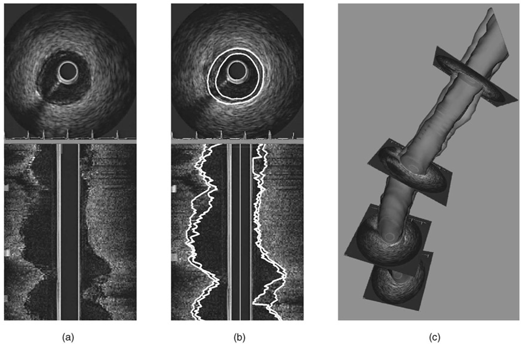
(a) Polar and longitude cross-sections of the original image. (b) Segmentation result by optimal coupled-surface segmentation. (c) Surface reconstruction.

8 DISCUSSION

In the following discussion, we focus on several important issues potentially influencing the utility of the presented method. First, the ability to incorporate geometric constraints into the surface detection process is considered. Second, the steps necessary allowing interactive guidance of the search process in difficult images are described. Finally, the proposed method is compared to the existing segmentation methods.

8.1 Variable Geometric Constraints

In the previous sections, homogeneous smoothness and separation constraints whose values remain constant along each axial direction were considered. In fact, the proposed algorithm allows incorporation of variable geometric constraints. The constraints can be specified adaptively based on the local image context. For example, the surface smoothness and surface-to-surface interrelations may vary at different locations. Variable geometric constraints can be incorporated into the algorithm by rearrangements of the graph edges. As a result, the graph arcs may no longer be parallel as the case in the constant-constraint case.

Nevertheless, there are practical obstacles that need to be overcome for this approach to become useful. For the variable-constraint setup, a key problem remains challenging: How to automatically adjust the constraints as needed. We expect that employing on-the-fly machine learning techniques will help solving this issue.

8.2 Surface Guidance and Interactive Segmentation

In practice, prior knowledge about the shape and/or position of the desired optimal surfaces may be available. Such knowledge can be incorporated into the algorithm by placing “landmark” points in the image, which are the voxels that the detected surfaces must pass through. There are essentially two ways to achieve this. One is by manipulating the cost values of the graph nodes corresponding to the landmark voxels, i.e., by assigning them an extremely low cost such that the feasible surface including these voxels will have the minimum cost globally. However, a more reliable and efficient way to incorporate landmarks would be to change the graph construction itself. It is clear that the (x, y)-column with a landmark node will contain only a single node corresponding to the landmark voxel. Due to the introduction of landmarks, some nodes in the original graph that do not satisfy the geometric relationship with the landmarks can be automatically pruned, further reducing the graph complexity. The placement of landmarks is especially useful in human-computer interactive segmentation.

8.3 Relations to the Open-Pit Mining Problem

The single surface segmentation algorithm is closely related to the open-pit mining problem [69], [70], [71], which seeks to excavate the earth surface to extract ore (e.g., gold) contained in the earth. Each block of earth is associated with a net profit, which is the value of the ore it contains minus the excavation cost of the block. A key objective in open-pit mining is to excavate earth blocks until a pit surface is reached such that the total net profit is maximized. Due to the use of the large mining machines, the pit surface is expected to be “smooth.”

8.4 Comparison to Other Segmentation Methods

In this paper, performance of our new method was directly compared with that of the dynamic programming in several medical image segmentation tasks. This is because of their common graph-based formulation and similar domain of application. In recent years, many novel and powerful techniques have blossomed in many aspects of imaging and vision. In this respect, the level set framework saw an especially fast development [39], [40]. Unfortunately, the fact that many of these techniques are application-specific and the unavailability of competing implementations that are optimized to the handy segmentation tasks make experimental comparisons infeasible. Nevertheless, the recently-discovered linkage [47] between level set methods and graph-cuts suggests that the latter approach would be preferred whenever the energy functions can be expressed in terms of graph models, such that optimal solutions can be efficiently computed.

Compared to other techniques, one of our major innovations is that, by considering only objects with certain shapes (i.e., terrain-like and cylindrical), the geometric constraints, which are crucial for medical image segmentations, can be modeled in a graph with nontrivial arc constructions. Thus, the geometric constraints become “hard” constraints that have intuitive geometric meanings, as opposed to “soft” constraints defined by weighted energy terms that simulate natural behaviors. The practical advantages are that the method becomes less image-dependent and the burden on objective function design and calibration is relieved. The smoothness thus modeled is not discontinuity-preserving, as desired by some other problems in vision (e.g., stereo, multicamera scene construction). However, discontinuity-preservation is more a curse than a blessing in medical images since typical objects are sufficiently smooth. Another advantage of our method is that it can be naturally generalized to handle multiple coupled surfaces. For the methods developed by Boykov and Jolly [33], [47], for instance, such an extension is nontrivial.

Some of the demonstrated problems were difficult to solve by existing techniques, e.g., the delineation of inner and outer airway wall surfaces in pulmonary CT image. Some others were previously tackled by using slice-by-slice or 3D model-based methods, including the detection of arterial wall and plaque from in vitro MR [68] and intravascular ultrasound (IVUS) images [6], [72], [73], segmentation of the endocardial and epicardial boundaries of the left ventricle from cardiac MR or CT [56], [74], and the extraction of diaphragm dome surface in CT data sets [75]. Our new approach has the potential of requiring less human interaction, yielding more accurate results and being more robust than the previous methods.

9 CONCLUSION

A polynomial-time algorithm for segmenting a single surface, or simultaneously segmenting multiple mutually-related surfaces in volumetric images has been developed and validated on phantoms and medical images. The method is efficient and robust. The resulting surfaces are globally optimal with respect to the employed objective function and geometric constraints. The surface smoothness and separation parameters provide a flexible means for modeling various inherent properties and interrelations of the desired surfaces. The method is readily extensible to higher dimensions.

Biographies

Kang Li received the BS degree from Nanjing University, China, in 2002 and the MS degree from the University of Iowa in 2003, both in electrical engineering. He is currently working toward the PhD degree in the Department of Electrical and Computer Engineering at the Carnegie Mellon University. His research interests are in biomedical image processing, computer vision, graph algorithms, and machine learning. He is a student member of the IEEE and the IEEE Computer Society.

Xiaodong Wu received the BS and MS degrees both in computer science from Peking University, China, in 1992 and 1995, respectively, and the PhD degree in computer science and engineering from the University of Notre Dame in August 2002. He is currently an assistant professor in the Departments of Electrical and Computer Engineering and Radiation Oncology at the University of Iowa. From 2002 to 2004, he was an assistant professor of computer science at the University of Texas—Pan American. His research interests are primarily in biomedical computing and computer algorithms with a particular emphasis on the development and implementation of efficient algorithms for solving challenging problems arising in computer-assisted medical diagnosis and treatment, biomedical image analysis, and bioinformatics. He is a senior member of the IEEE.

Danny Z. Chen received the BS degree in computer science and mathematics from the University of San Francisco, San Francisco, California, in 1985 and the MS and PhD degrees in computer science from Purdue University, West Lafayette, Indiana, in 1988 and 1992, respectively. He is a professor in the Department of Computer Science and Engineering at the University of Notre Dame. In 1996, he received the Faculty Early Career Development (CAREER) Award from the US National Science Foundation. His research interests include parallel computing, computational geometry, algorithms, and data structures. He is a senior member of the IEEE.

Milan Sonka received the PhD degree in 1983 from the Czech Technical University in Prague. He is a professor of electrical and computer engineering at the University of Iowa and a fellow of the IEEE. His research interests include medical imaging and knowledge-based image analysis. A major focus of his research in the last several years has been on the development of clinically applicable automated techniques for cardiovascular analysis, pulmonary CT image analysis, cell tracking and cellular shape analysis, and augmented reality image-based surgical planning. He is the first author of the book Image Processing, Analysis and Machine Vision published in 1993 by Chapman and Hall in London, second edition 1998 by PWS, Pacific Grove, California. He has coauthored or coedited 10 other books including the Handbook of Medical Imaging, Volume II—Medical Image Processing and Analysis published in 2000. He has authored seven book chapters, more than 60 journal papers, 160 conference papers, and 60 abstracts. He is associate editor of the IEEE Transactions on Medical Imaging and member of the editorial board of the International Journal of Cardiovascular Imaging.

REFERENCES

- 1.Montanari U. On the Optimal Detection of Curves in Noisy Pictures. Comm. ACM. 1971 May;vol. 14:335–345. [Google Scholar]
- 2.Martelli A. Edge Detection Using Heuristic Search Methods. Computer Graphics and Image Processing. 1972 Aug.vol. 1:169–182. [Google Scholar]
- 3.Martelli A. An Application of Heuristic Search Methods to Edge and Contour Detection. Comm. ACM. 1976 Feb.vol. 19:73–83. [Google Scholar]
- 4.Pope D, Parker D, Clayton P, Gustafson D. Left Ventricular Border Detection Using a Dynamic Search. Radiology. 1985 May;vol. 155:513–518. doi: 10.1148/radiology.155.2.3885315. [DOI] [PubMed] [Google Scholar]
- 5.Schenk A, Prause G, Peitgen H-O. Local Cost Computation for Efficient Segmentation of 3D Objects with Live Wire; Proc. SPIE Int’l Symp. Medical Imaging: Image Processing; 2001. pp. 1357–1364. [Google Scholar]
- 6.Sonka M, Zhang X, DeJong S, Collins S, McKay C. Segmentation of Intravascular Ultrasound Images: A Knowledge-Based Approach. IEEE Trans. Medical Imaging. 1995 Aug.vol. 14:719–732. doi: 10.1109/42.476113. [DOI] [PubMed] [Google Scholar]
- 7.Falcão AX, Udupa JK, Miyazawa FK. An Ultra-Fast User-Steered Image Segmentation Paradigm: Live Wire on the Fly. IEEE Trans. Medical Imaging. 2000 Jan.vol. 19 doi: 10.1109/42.832960. [DOI] [PubMed] [Google Scholar]
- 8.Thedens D, Skorton D, Fleagle S. Three-Dimensional Graph Searching Technique for Cardiac Border Detection in Sequential Images and Its Application to Magnetic Resonance Image Data. Computers in Cardiology. 1990 Sept.:57–60. [Google Scholar]
- 9.Thedens DR, Skorton DJ, Fleagle SR. Methods of Graph Searching for Border Detection in Image Sequences with Applications to Cardiac Magnetic Resonance Imaging. IEEE Trans. Medical Imaging. 1995;vol. 14(no 1):42–55. doi: 10.1109/42.370401. [DOI] [PubMed] [Google Scholar]
- 10.Frank R. master’s thesis. Univ. of Iowa; 1996. Optimal Surface Detection Using Multi-Dimensional Graph Search: Applications to Intravascular Ultrasound. [Google Scholar]
- 11.Falcão AX, Udupa JK. Segmentation of 3D Objects Using Live Wire; Proc. SPIE Int’l Symp. Medical Imaging: Image Processing; 1997. Apr., pp. 228–235. [Google Scholar]
- 12.Falcão AX, Udupa JK. A 3D Generalization of User-Steered Live-Wire Segmentation. Medical Image Analysis. 2000 Dec.vol. 4:389–402. doi: 10.1016/s1361-8415(00)00023-2. [DOI] [PubMed] [Google Scholar]
- 13.Wu X, Chen DZ. Optimal Net Surface Problems with Applications; Proc. 29th Int’l Colloquium Automata, Languages, and Programming (ICALP); 2002. Jul, pp. 1029–1042. [Google Scholar]
- 14.Li K, Wu X, Chen DZ, Sonka M. Efficient Optimal Surface Detection: Theory, Implementation and Experimental Validation; Proc. SPIE Int’l Symp. Medical Imaging: Image Processing; 2004. May, pp. 620–627. [Google Scholar]
- 15.Li K, Wu X, Chen DZ, Sonka M. Globally Optimal Segmentation of Interacting Surfaces with Geometric Constraints; Proc. IEEE CS Conf. Computer Vision and Pattern Recognition (CVPR); 2004. Jun, pp. 394–399. [Google Scholar]
- 16.Zahn C. Graph-Theoretic Methods for Detecting and Describing Gestalt Clusters. IEEE Trans. Computers. 1971;vol. 20:68–86. [Google Scholar]
- 17.Xu Y, Olman V, Uberbacher E. A Segmentation Algorithm for Noisy Images; Proc. IEEE Int’l Joint Symp. Intelligence and Systems; 1996. Nov., pp. 220–226. [Google Scholar]
- 18.Xu Y, Uberbacher EC. 2-D Image Segmentation Using Minimum Spanning Trees. Image and Vision Computing. 1997;vol. 15(no 1):47–57. [Google Scholar]
- 19.Jagannathan A, Miller E. A Graph-Theoretic Approach to Multiscale Texture Segmentation; Proc. Int’l Conf. Image Processing; 2002. Sept., pp. 777–780. [Google Scholar]
- 20.Felzenszwalb PF, Huttenlocher DP. Efficient Graph-Based Image Segmentation. Int’l J. Computer Vision. 2004 Sept.vol. 59:167–181. [Google Scholar]
- 21.Udupa JK, Samarasekera S. Fuzzy Connectedness and Object Definition: Theory, Algorithms, and Applications in Image Segmentation. Graphics Models and Image Processing. 1996 May;vol. 58:246–261. [Google Scholar]
- 22.Saha PK, Udupa JK. Relative Fuzzy Connectedness among Multiple Objects: Theory, Algorithms, and Applications in Image Segmentation. Computer Vision and Image Understanding. 2000;vol. 82:42–56. doi: 10.1016/j.cviu.2006.10.005. [DOI] [PMC free article] [PubMed] [Google Scholar]
- 23.Nyul LG, Falcão AX, Udupa JK. Fuzzy-Connected 3D Image Segmentation at Interactive Speeds. Graphical Models. 2002 Sept.vol. 64:259–281. [Google Scholar]
- 24.Falcão AX, Stolfi J, de Alencar Lotufo R. The Image Foresting Transform: Theory, Algorithms, and Applications. IEEE Trans. Pattern Analysis and Machine Intelligence. 2004 Jan.vol. 26(no 1):19–29. doi: 10.1109/tpami.2004.1261076. [DOI] [PubMed] [Google Scholar]
- 25.Reiber JHC, van der Zwet PMJ, von Land CD, Loois G, Zorn I, van den Brand M, Gerbrands JJ. On-Line Quantification of Coronary Angiograms with the DCI System. Medicamundi. 1989;vol. 34:89–98. [Google Scholar]
- 26.Sonka M, Winniford MD, Collins SM. Robust Simultaneous Detection of Coronary Borders in Complex Images. IEEE Trans. Medical Imaging. 1995 Mar.vol. 14:151–161. doi: 10.1109/42.370412. [DOI] [PubMed] [Google Scholar]
- 27.Sonka M, Hlavac V, Boyle R. Image Processing, Analysis, and Machine Vision. second ed. Brooks/Cole Publishing Company; 1999. [Google Scholar]
- 28.Wu Z, Leahy R. An Optimal Graph Theoretic Approach to Data Clustering: Theory and Its Application to Image Segmentation. IEEE Trans. Pattern Analysis Machine Intelligence. 1993 Nov.vol. 15(no 11):1101–1113. [Google Scholar]
- 29.Cox I, Rao S, Zhong Y. Ratio Regions: A Technique for Image Segmentation; Proc. Int’l Conf. Pattern Recognition; 1996. Aug., pp. 557–564. [Google Scholar]
- 30.Ishikawa H, Geiger D. Segmentation by Grouping Junctions; Proc. IEEE Conf. Computer Vision and Pattern Recognition; 1998. Jun, pp. 125–131. [Google Scholar]
- 31.Jermyn I, Ishikawa H. Globally Optimal Regions and Boundaries as Minimum Ratio Cycles. IEEE Trans. Pattern Analysis and Machine Intelligence. 2001 Oct.vol. 23(no 10):1075–1088. [Google Scholar]
- 32.Shi J, Malik J. Normalized Cuts and Image Segmentation. IEEE Trans. Pattern Analysis Machine Intelligence. 2000 Aug.vol. 22(no 8):888–905. [Google Scholar]
- 33.Boykov Y, Jolly M-P. Interactive Organ Segmentation Using Graph Cuts. Proc. Medical Image Computing and Computer-Assisted Intervention (MICCAI) 2000:276–286. [Google Scholar]
- 34.Boykov YY, Jolly M-P. Interactive Graph Cuts for Optimal Boundary and Region Segmentation of Objects in N-D Images; Proc. Int’l Conf. Computer Vision (ICCV); 2001. Jul, pp. 105–112. [Google Scholar]
- 35.Wang S, Siskind J. Image Segmentation with Ratio Cut. IEEE Trans. Pattern Analysis and Machine Intelligence. 2003 June;vol. 25(no 6):675–690. [Google Scholar]
- 36.Boykov Y, Kolmogorov V. An Experimental Comparison of Min-Cut/Max-Flow Algorithms for Energy Minimization in Vision. IEEE Trans. Pattern Analysis and Machine Intelligence. 2004 Sept.vol. 26(no 9):1124–1137. doi: 10.1109/TPAMI.2004.60. [DOI] [PubMed] [Google Scholar]
- 37.Li Y, Sun J, Tang C-K, Shum H-Y. Lazy Snapping. ACM Trans. Graphics (TOG) 2004 Aug.vol. 23:303–308. [Google Scholar]
- 38.Kim J, Zabih R. A Segmentation Algorithm for Contrast-Enhanced Images; Proc. IEEE Int’l Conf. Computer Vision; 2003. Oct., pp. 502–509. [Google Scholar]
- 39.Sethian J. Level Set Methods and Fast Marching Methods Evolving Interfaces in Computational Geometry, Fluid Mechanics, Computer Vision, and Materials Science. second ed. Cambridge, U.K: Cambridge Univ. Press; 1999. [Google Scholar]
- 40.Osher S, Paragios N, editors. Geometric Level Set Methods in Imaging, Vision and Graphics. Springer; 2003. [Google Scholar]
- 41.Boykov Y, Veksler O, Zabih R. Fast Approximate Energy Minimization via Graph Cuts. IEEE Trans. Pattern Analysis and Machine Intelligence. 2001 Nov.vol. 23(no 11):1222–1239. [Google Scholar]
- 42.Kolmogorov V, Zabih R. What Energy Functions Can Be Minimized via Graph Cuts? IEEE Trans. Pattern Analysis and Machine Intelligence. 2004 Feb.vol. 26(no 2):147–159. doi: 10.1109/TPAMI.2004.1262177. [DOI] [PubMed] [Google Scholar]
- 43.Geman S, Geman D. Stochastic Relaxation, Gibbs Distributions, and the Bayesian Restoration of Images. IEEE Trans. Pattern Analysis and Machine Intelligence. 1984 Nov.vol. 6:721–741. doi: 10.1109/tpami.1984.4767596. [DOI] [PubMed] [Google Scholar]
- 44.Ford LRJ, Fulkerson DR. Maximal Flow through a Network. Canadian J. Math. 1956;vol. 8:399–404. [Google Scholar]
- 45.Goldberg AV, Tarjan RE. A New Approach to the Maximum-Flow Problem. J. ACM. 1988;vol. 35:921–940. [Google Scholar]
- 46.Goldberg AV, Rao S. Beyond the Flow Decomposition Barrier. J. ACM. 1998;vol. 45:783–797. [Google Scholar]
- 47.Boykov Y, Kolmogorov V. Computing Geodesics and Minimal Surfaces Via Graph Cuts; Proc. Int’l Conf. Computer Vision (ICCV); 2003. Oct., pp. 26–33. [Google Scholar]
- 48.Zeng X, Staib L, Schultz R, Duncan J. Segmentation and Measurement of the Cortex from 3-D MR Images Using Coupled-Surfaces Propagation. IEEE Trans. Medical Imaging. 1999 Oct.vol. 18:927–937. doi: 10.1109/42.811276. [DOI] [PubMed] [Google Scholar]
- 49.MacDonald D, Kabani N, Avis D, Evans A. Automated 3-D Extraction of Inner and Outer Surfaces of Cerebral Cortex from MRI. NeuroImage. 2000 Sept.vol. 12(no 3):340–356. doi: 10.1006/nimg.1999.0534. [DOI] [PubMed] [Google Scholar]
- 50.Goldenberg R, Kimmel R, Rivlin E, Rudzsky M. Cortex Segmentation: A Fast Variational Geometric Approach. IEEE Trans. Medical Imaging. 2002 Dec.vol. 21:1544–1551. doi: 10.1109/TMI.2002.806594. [DOI] [PubMed] [Google Scholar]
- 51.Spreeuwers L, Breeuwer M. Detection of Left Ventricular Epi- and Endocardial Borders Using Coupled Active Contours. Computer Assisted Radiology and Surgery. 2003 June;:1147–1152. [Google Scholar]
- 52.Goldenberg R, Kimmel R, Rivlin E, Rudzsky M. Fast Geodesic Active Contours. IEEE Trans. Image Processing. 2001 Oct.vol. 10:1467–1475. doi: 10.1109/83.951533. [DOI] [PubMed] [Google Scholar]
- 53.Han X, Xu C, Prince JL. A Topology Preserving Level Set Method for Geometric Deformable Models. IEEE Trans. Pattern Analysis and Machine Intelligence. 2003 June;vol. 25(no 6):755–768. [Google Scholar]
- 54.Cootes TF, Hill A, Taylor CJ, Haslam J. The Use of Active Shape Models for Locating Structures in Medical Images; Proc. 13th Int’l Conf. Information Processing in Medical Imaging (IPMI); 1993. pp. 33–47. [Google Scholar]
- 55.Cootes T, Edwards G, Taylor C. Active Appearance Models. IEEE Trans. Pattern Analysis and Machine Intelligence. 2001 June;vol. 23(no 6):681–685. [Google Scholar]
- 56.Mitchell S, Lelieveldt B, van der Geest R, Bosch H, Reiber J, Sonka M. Multistage Hybrid Active Appearance Model Matching: Segmentation of Left and Right Ventricles in Cardiac MR Images. IEEE Trans. Medical Imaging. 2001 May;vol. 20:415–423. doi: 10.1109/42.925294. [DOI] [PubMed] [Google Scholar]
- 57.Hochbaum D. A New-Old Algorithm for Minimum-Cut and Maximum-Flow in Closure Graphs. Networks. 2001;vol. 37:171–193. [Google Scholar]
- 58.Picard J. Maximal Closure of a Graph and Applications to Combinatorial Problems. Management Science. 1976;vol. 22:1268–1272. [Google Scholar]
- 59.Sonka M, Reddy GK, Winniford MD, Collins SM. Adaptive Approach to Accurate Analysis of Small-Diameter Vessels in Cineangiograms. IEEE Trans. Medical Imaging. 1997 Feb.vol. 16:87–95. doi: 10.1109/42.552058. [DOI] [PubMed] [Google Scholar]
- 60.Mumford D, Shah J. Optimal Approximation by Piecewise Smooth Functions and Associated Variational Problems. Comm. Pure and Applied Math. 1989;vol. 42:577–685. [Google Scholar]
- 61.Chan TF, Vese LA. Active Contour without Edges. IEEE Trans. Image Processing. 2001 Feb.vol. 10(no 2):266–277. doi: 10.1109/83.902291. [DOI] [PubMed] [Google Scholar]
- 62.Tschirren J. PhD dissertation. Univ. of Iowa; 2003. Aug., Segmentation, Anatomical Labeling, Branch-Point Matching, and Quantitative Analysis of Human Airway in Volumetric CT Images. [Google Scholar]
- 63.Palágyi K, Sorantin E, Balogh E, Kuba A, Halmai C, Erdohelyi B, Hausegger K. A Sequential 3D Thinning Algorithm and Its Medical Applications; Proc. 17th Int’l Conf. Information Processing in Medical Imaging (IPMI); 2001. pp. 409–415. [Google Scholar]
- 64.Unser M, Aldroudi A, Eden M. B-Spline Signal Processing: Part I—Theory. IEEE Trans. Signal Processing. 1993 Feb.vol. 41:821–833. [Google Scholar]
- 65.Unser M, Aldroubi A, Eden M. B-Spline Signal Processing: Part II—Efficient Design and Applications. IEEE Trans. Signal Processing. 1993 Feb.vol. 41(no 2):834–848. [Google Scholar]
- 66.Cherkassky B, Goldberg A. On Implementing Push-Relabel Method for the Maximum Flow Problem. Algorithmica. 1997;vol. 19:390–410. [Google Scholar]
- 67.Huang X, Metaxas D, Chen T. Metamorphs: Deformable Shape and Texture Models; Proc. IEEE CS Conf. Computer Vision and Pattern Recognition (CVPR); 2004. Jun, pp. 496–503. [Google Scholar]
- 68.Yang F, Holzapfel G, Schulze-Bauer C, Stollberger R, Thedens D, Bolinger L, Stolpen A, Sonka M. Segmentation of Wall and Plaque in in Vitro Vascular MR Images. The Int’l J. Cardiac Imaging. 2003 Oct.vol. 19:419–428. doi: 10.1023/a:1025829232098. [DOI] [PubMed] [Google Scholar]
- 69.Lerchs IGH. Optimum Design of Open-Pit Mines. Trans. CIM. 1965;vol. 58:17–24. [Google Scholar]
- 70.Denby B, Schofield D. Genetic Algorithms: A New Approach to Pit Optimization; Proc. 24th Int’l APCOM Symp; 1993. pp. 126–133. [Google Scholar]
- 71.Hochbaum D, Chen A. Improved Planning for the Open—Pit Mining Problem. Operations Research. 2000;vol. 48:894–914. [Google Scholar]
- 72.Zhang X, McKay C, Sonka M. Tissue Characterization in Intravascular Ultrasound Images. IEEE Trans. Medical Imaging. 1998 Dec.vol. 17:889–899. doi: 10.1109/42.746622. [DOI] [PubMed] [Google Scholar]
- 73.Coşkun AÜ, Yeghiazarians Y, Kinlay S, Clark ME, Ilegbusi OJ, Wahle A, Sonka M, Popma JJ, Kuntz RE, Feldman CL, Stone PH. Reproducibility of Coronary Lumen, Plaque, and Vessel Wall Reconstruction and of Endothelial Shear Stress Measurements In-Vivo in Humans. Catheterization and Cardiovascular Interventions. 2003 Sept.vol. 60(no 1):63–78. doi: 10.1002/ccd.10594. [DOI] [PubMed] [Google Scholar]
- 74.Mitchell S, Bosch J, Lelieveldt B, van der Geest R, Reiber J, Sonka M. 3-D Active Appearance Models: Segmentation of Cardiac MR and Ultrasound Images. IEEE Trans. Medical Imaging. 2002 Sept.vol. 21:1167–1178. doi: 10.1109/TMI.2002.804425. [DOI] [PubMed] [Google Scholar]
- 75.Beichel R, Gotschuli G, Sorantin E, Leberl FW, Sonka M. Diaphragm Dome Surface Segmentation in CT Data Sets: A 3D Active Appearance Model Approach; Proc. SPIE Int’l Symp. Medical Imaging: Image Processing; 2002. May, pp. 475–484. [Google Scholar]