

Abstract
In the application of hypercapnic normalization to functional magnetic resonance imaging (fMRI) studies, the blood oxygenation level dependent (BOLD) response to a functional stimulus is typically divided by the BOLD response to a hypercapnic challenge. While some prior studies have shown that hypercapnic normalization can reduce inter-subject BOLD variability, other studies have found an increase in inter-subject variability. In this study we used measures of baseline cerebral blood flow (CBF) and the functional BOLD and CBF responses to both visual stimuli and hypercapnia to assess the effect of hypercapnic normalization on inter-subject variability. We found that the functional and hypercapnic BOLD and CBF responses all exhibited a significant inverse dependence on baseline CBF. In contrast, the maximum BOLD response was independent of baseline CBF and was not a major source of inter-subject BOLD variability. Division of the functional BOLD response by the hypercapnic BOLD response increased inter-subject variability in the normalized responses as compared to the original responses, reflecting the presence of a systematic bias term that was inversely dependent on the hypercapnic BOLD response. This systematic bias resulted from a positive intercept term in the linear relationship between the functional and hypercapnic BOLD responses. This positive intercept term reflected a steeper inverse dependence of the hypercapnic CBF response on baseline CBF, as compared to the functional CBF response. In contrast to the results obtained with normalization based on division, normalized responses obtained by using the hypercapnic BOLD response as a covariate were unaffected by the systematic bias and exhibited reduced inter-subject variability. The findings of this study indicate that the positive intercept in the linear relationship between functional and hypercapnic BOLD responses should be carefully considered in the hypercapnic normalization of BOLD fMRI data.
Introduction
Over the past decade, blood oxygenation level dependent (BOLD) functional MRI (fMRI) has become a powerful tool for non-invasive studies of the working human brain. Although the BOLD signal is widely regarded as a measure of neural activity, it reflects changes in a number of physiological variables, namely cerebral blood volume (CBV), cerebral blood flow, and cerebral oxygen metabolism (Buxton 2002). As a result, differences between subjects in factors unrelated to neural activity, such as vascular reactivity or hematocrit levels, can lead to significant inter-subject variability in the BOLD response (D’Esposito et al. 2003; Gustard et al. 2003; Handwerker et al. 2007). In this paper we use the term inter-subject variability to refer to the coefficient of variation (i.e. standard deviation divided by the mean) of the BOLD signal amplitude observed across a sample of subjects. Increased inter-subject variability can reduce the statistical power of fMRI studies, necessitating larger sample sizes with accompanying increased cost. A method that reduces BOLD inter-subject variability due to non-neural factors would be of great use, especially for studies in which the sample size may be limited.
Hypercapnic normalization refers to the division of the functional BOLD response by the BOLD response to mild hypercapnia in each voxel, where hypercapnia is induced by either the administration of carbon dioxide or a voluntary breathhold (Bandettini and Wong 1997). It is generally assumed that the mild hypercapnic stimuli has a minimal effect on neural activity and oxygen metabolism (Jones et al. 2005; Sicard and Duong 2005; Zappe et al. 2008), so that the hypercapnic BOLD response primarily reflects changes in cerebral blood flow, as well as other factors such as magnetic field strength and baseline cerebral blood volume. As these non-neural factors are either similar or identical for the functional and hypercapnic BOLD responses, division of the two responses can reduce the variability due to these factors. (Bandettini and Wong 1997) first used hypercapnic normalization to reduce BOLD variability associated with differences in resting cerebral blood volume across the brain. (Cohen et al. 2004) performed a similar procedure using subjects scanned with several protocols (i.e. different pulse sequences and magnetic field strengths) and found that hypercapnic normalization reduced the sensitivity to different scan protocols and magnetic field strengths. However, the results of that study showed that hypercapnic normalization increased inter-subject variability of the BOLD responses. In a study of aging, (Handwerker et al. 2007) demonstrated that hypercapnic normalization of a visuomotor saccade task by a breath-hold task removed significant age-related differences in two brain regions (frontal and supplementary eye fields). These reductions in inter-group differences were accompanied by increased inter-subject variability in the older subject group. In contrast, two recent studies have reported a decrease in inter-subject variability after hypercapnic normalization using a breath-hold challenge that was applied to the functional responses to a working memory task (Thomason et al. 2007) and a motor task (Biswal et al. 2007). The mixed results of these prior studies indicate the need for a better understanding of hypercapnic normalization’s effect on inter-subject variability.
In this paper, we take a combined theoretical and experimental approach to examine in detail the effect of hypercapnic normalization on inter-subject variability. We begin in the Theory section by demonstrating how the presence of a positive intercept in the linear relationship between the functional and hypercapnic BOLD responses can lead to a systematic bias term that increases inter-subject variability in the normalized responses. We then use a mathematical model of the BOLD signal to better understand the origin of this positive intercept term and its relation to other physiological quantities.
In the experimental portion of this study, we use arterial spin labeling MRI to acquire measures of baseline CBF and of the functional BOLD and CBF responses to both visual stimulus and hypercapnia. With these experimental measures, we confirm our theoretical prediction that the presence of an intercept term in the relation between functional and hypercapnic BOLD responses can lead to increased variability in the normalized responses. We also integrate the experimental measures with the BOLD signal model presented in the Theory section to demonstrate the dependence of the intercept term on the functional and hypercapnic CBF responses. Finally, we consider an alternative method for hypercapnic normalization in which the hypercapnic BOLD response is used as a covariate.
Theory
In this section, we first show that the presence of a non-zero intercept in the linear relation between the functional and hypercapnic BOLD responses results in a systematic bias term in the normalized responses. We then show that normalized responses computed by division on a per-voxel basis or on a per-subject basis are similar. We conclude by using a BOLD signal model to determine the physical meaning of the normalized responses.
The Intercept in the Relation Between Functional and Hypercapnic BOLD Responses Results in a Systematic Bias Term in the Normalized Responses
Prior studies have noted a linear relation between the average functional BOLD responses Bi and the hypercapnic BOLD responses BH,i observed across a sample of healthy subjects (Handwerker et al. 2007; Thomason et al. 2007) of the form:
| (1) |
where A is the group slope, G is the group intercept, Ei is the residual to the linear fit, and the subscript i indicates the ith subject. Examples of this relation are shown in Figure 1 (panels c and d). Normalizing by the subject average hypercapnic responses produces the normalized response for each subject of the form:
| (2) |
which is the sum of (a) the slope A between the functional and hypercapnic responses, (b) a systematic bias term G/BH,i that is inversely proportional to BH,i, and (c) a residual term Ei/BH,i. Note that the bias term G/BH,i represents systematic variability that is not eliminated by the hypercapnic normalization process. Examples of this systematic bias in the normalized response are shown in Figure 3 (panels b and f).
Figure 1.
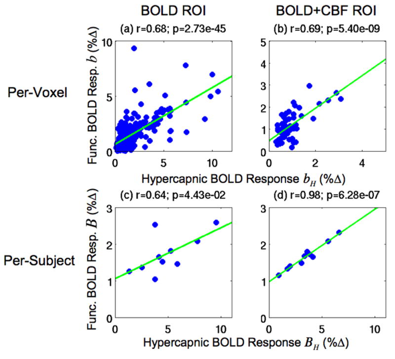
Scatter plots of the per-voxel functional BOLD responses b versus the hypercapnic BOLD responses bH in Subject 1 (top row) and the per-subject functional BOLD responses B versus hypercapnic BOLD responses BH (bottom row). Responses are from the BOLD ROI (left column) and the BOLD+CBF ROI (right column). Green lines indicate linear fits.
Figure 3.

Scatter plots of the functional BOLD responses and the normalized responses versus the hypercapnic BOLD responses. The first column shows scatter plots of the functional BOLD responses B vs. the hypercapnic BOLD responses BH. The remaining columns show scatter plots of the normalized responses (B̂, B″, and B̂cov) versus the hypercapnic BOLD responses BH. Second column: the per-subject normalized responses B̂. Third column: the per-voxel normalized responses B″. Fourth column: the covariate normalized responses B̂cov. Values are shown for the BOLD ROI (top row) and BOLD+CBF ROI (bottom row). Green lines indicate linear fits.
Hypercapnic Normalization on a Per-voxel Basis versus a Per-subject Basis
In the previous section, we showed that normalization using the subject average hypercapnic BOLD responses BH,i can result in a systematic bias term G/BH,i in the normalized response B̂i when the normalization is performed on a per-subject basis. To date, most normalization approaches have divided the functional BOLD response bi, j in each voxel by the corresponding hypercapnic response bH,i, j in that voxel, where the subscripts i and j denote the ith subject and jth voxel, respectively (Bandettini and Wong 1997; Cohen et al. 2004; Biswal et al. 2007; Handwerker et al. 2007; Thomason et al. 2007). Averaging the per-voxel normalized responses bi, j/bH,i, j across a region-of-interest (ROI) yields an average response for each subject of the form:
| (3) |
where Ni is the number of voxels in the ROI. In other words, represents the average subject response obtained when normalization is performed on a per-voxel basis prior to averaging over the ROI, while B̂i in Eqn. 2 is the average response obtained when averaging of the functional and hypercapnic responses over the ROI is performed prior to normalization, which is then done a per-subject basis.
To determine the relation between the two types of normalized responses (B̂i and ), we make use of the linear relationship between bi, j and bH,i, j that has been demonstrated in previous studies (Bandettini and Wong 1997; Cohen et al. 2004; Biswal et al. 2007; Handwerker et al. 2007; Thomason et al. 2007). The relation has the form:
| (4) |
where ai is the subject slope, gi is the subject intercept, and ei,j is the residual to the linear fit. Examples of this relation are shown in Figure 1 (panels a and b). We show in Appendix A that the linear relation in Eqn. 4 yields the following relation between and B̂i:
| (5) |
The two normalized responses differ only by the subject dependent term . We find empirically that this subject dependent term is positive and is about 25% of the average per-voxel normalized response B″ and 33% of the average per-subject normalized response B̂ as shown in the Results and Figure 2. This reflects the empirical findings that the intercept gi is approximately equal to 1 across subjects and the difference between the two summation terms is positive and less than one, where is about twice as large as (See also Results). For the remaining theoretical development, we will adopt the subject average form B̂i because its usage simplifies the presentation for studies of inter-subject variability. Note however, that as expected from Eqn. 5, the experimental results obtained using both forms are similar, as shown in Figures 2 and 3 of the Results section.
Figure 2.
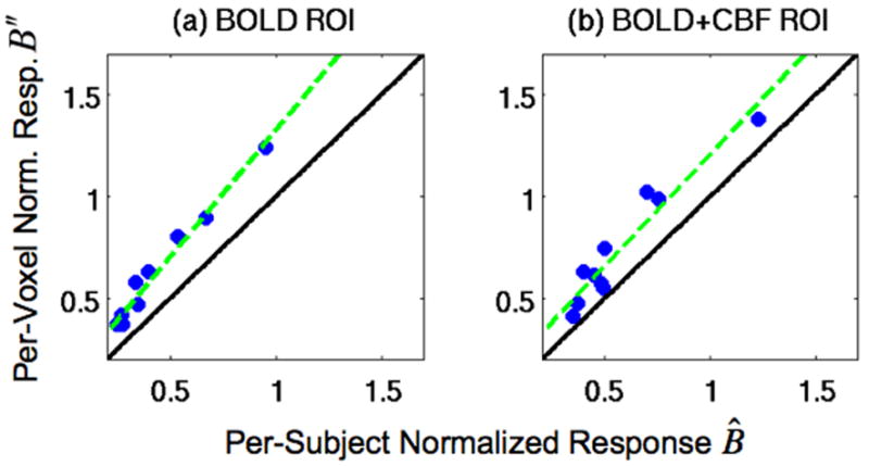
Scatter plots of the per-voxel normalized responses B″ versus the per-subject normalized responses B̂ in (a) the BOLD ROI and (b) the BOLD+CBF ROI. Black diagonal lines are the lines of equality, and the green lines are linear fits. The location of data points above the lines of equality (black lines) are consistent with the finding that the per-voxel normalized responses B″ were significantly larger than the per-subject normalized responses B̂ (p<0.001). The significant correlations between the per-voxel normalized responses B″ and the per-subject normalized responses B̂ (p<0.001) are demonstrated by the overlap of the linear fits (green lines) with the data points.
Physical Meanings of Normalized Response Components
As shown in Eqn. 2, the presence of a non-zero intercept term G gives rise to a systematic bias term G/H,i. In this section, we use the BOLD signal model introduced by (Davis et al. 1998) to show that the intercept term G depends on the relation between the functional and hypercapnic CBF responses. We also show that the empirically observed linear relation between Bi and BH,i (Eqn. 1) is consistent with the Davis Model. The Davis Model can be written as:
| (6) |
where is the maximum attainable percent BOLD response, TE is the echo time, Pi is a scan dependent scaling term, CBV0,i is the resting cerebral blood volume, [dHbi]v0 is the venous deoxyhemoglobin concentration, and the subscript v0 indicates the resting-state venous value. In addition, Fi is the percent CBF response to a functional task, mi is the percent cerebral oxygen metabolism response (CMRO2) to a functional task, α is Grubb’s exponent (Grubb et al. 1974), and β is an exponent that depends primarily on vessel size and magnetic field strength (Davis et al. 1998). With hypercapnia, it is typically assumed that mi = 0 (Davis et al. 1998; Hoge et al. 1999), so that the hypercapnic BOLD response is modeled as:
| (7) |
where the subscript H denotes the hypercapnic condition. From Eqns. 6 and 7, we can see that the relation between Bi and BH,i will depend on the relation between the functional and hypercapnic CBF responses, Fi and FH,i, and also the coupling between Fi and mi.
To proceed, we make use of the following experimental observations obtained for the sample of healthy young subjects in the present study (see Results and Figures 4 and 5): 1) the maximum BOLD response Mi is relatively constant across subjects, 2) the CBF/CMRO2 coupling ratio n = Fi/mi is relatively constant across subjects, and 3) the functional CBF response Fi is linearly related to the hypercapnic CBF response FH,i, that is Fi = c1 · FH,i + c2, where c1 is the group slope and c2 is the group intercept. Combining these observations with Eqns. 6 and 7, we show in Appendix B that the intercept term in the Eqn. 2 is given by:
| (8) |
and the slope is:
| (9) |
where FHM is the maximum hypercapnic CBF response observed across the group. As shown in Appendix B and Figure 6, the nonlinear relation between Bi and BH,i is fairly well approximated by a linear relation (Eqn. 1) with intercept G and approximate slope A as defined in Eqns 8 and 9.
Figure 4.
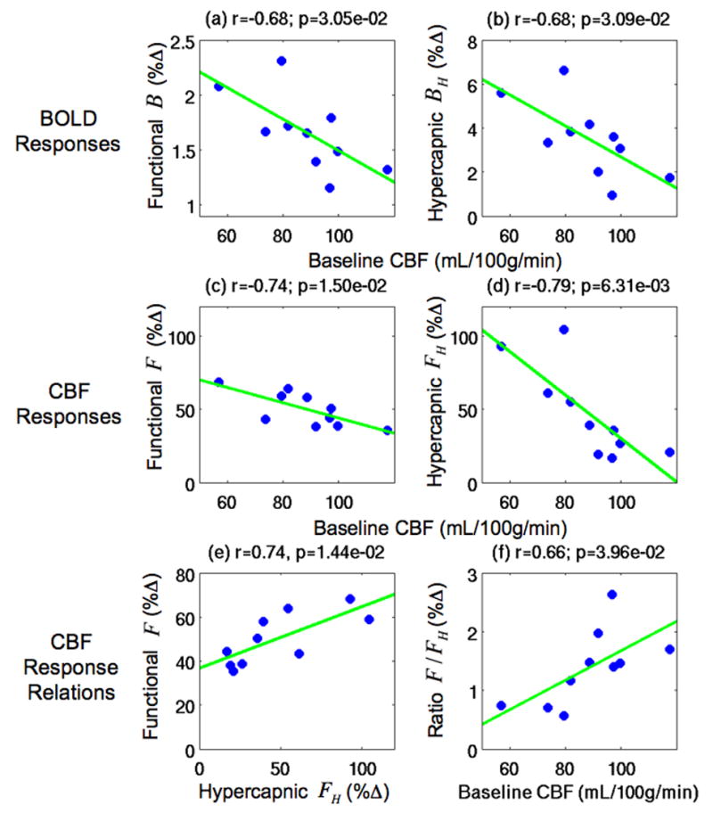
Scatter plots showing the dependence of the BOLD and CBF responses on baseline CBF in the BOLD+CBF ROI. Top row: Scatter plots of a) the functional BOLD responses B and (b) the hypercapnic BOLD responses BH versus baseline CBF. Second row: Scatter plots of (c) the functional CBF responses F and (d) the hypercapnic CBF responses FH versus baseline CBF. Third row: (e) the functional CBF responses F versus the hypercapnic CBF responses FH and (f) ratio of the functional and hypercapnic CBF responses F/FH versus baseline CBF. Green lines indicate linear fits. Baseline CBF values were significantly correlated (p<0.04) to the BOLD responses (B and BH), the CBF responses (F and FH), and the ratio of the functional and hypercapnic CBF responses F/FH. Also, the functional CBF responses F were significantly correlated to the hypercapnic CBF responses FH (p=0.014).
Figure 5.
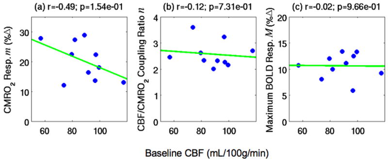
Scatter plots of estimated BOLD signal model parameters versus baseline CBF in the BOLD+CBF ROI: (a) the cerebral oxygen metabolism (CMRO2) responses m, (b) the CBF/CMRO2 coupling ratios n, and (c) the maximum BOLD responses M. None of the BOLD model parameters shown were significantly correlated to baseline CBF.
Figure 6.
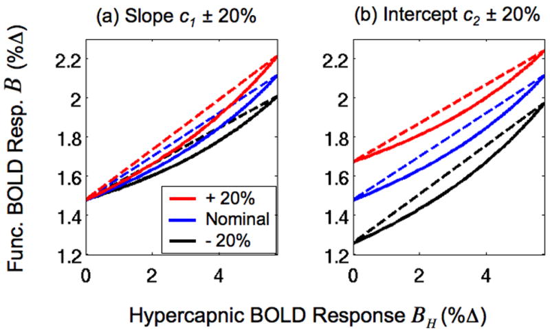
Predicted functional BOLD responses B versus hypercapnic BOLD responses BH. Responses were computed using a BOLD signal model (Eqns. B.1 and 7) with experimental and published values (solid blue line in both panels). The CBF slope c1 and intercept c2 parameter values estimated from the sample were used for the blue lines. In panel (a), the slope c1 was increased or decreased by 20% for the solid red and black lines, respectively. In panel (b) the intercept c2 was increased or decreased by 20% for the solid red and black lines, respectively. Dashed lines are linear approximations of the solid lines obtained using the intercept and slope expressions derived in Appendix B.
From Eqn. 8, we can see that the intercept G is non-zero whenever c2 is not equal to zero. In other words, a non-zero intercept G in the Bi vs. BH,i relation reflects the presence of a non-zero intercept in the Fi vs. FH,i relation (see Discussion section).
Methods
Experimental Protocol
Data presented here were also used for separate analyses examining a caffeine dose’s effect on metabolism (Perthen et al. 2008) and functional activation extents (Liau et al. 2008), and the experimental protocol is repeated here for convenience. Ten healthy adult subjects (5 males, mean age 33±7 years) participated in the study after giving informed consent. During each imaging session, subjects were presented with a stimulus consisting of “on” periods of an 8Hz full-field, full-contrast flashing checkerboard pattern with a small white square in the center. Inside the square, the numbers (2-4-3-5) appeared sequentially at 2Hz. The “off” periods were of equal luminance to the on periods and consisted of a gray background with a white square in the middle. Subjects were instructed to fixate on the white square at all times and press buttons on a 4-button response box with their right hand in accordance to the numbers. The flashing checkerboard was intended to activate the visual cortex while the motor task maintained subject attention. Each session consisted of the following arterial spin labeling (ASL) scans: 1) a resting-state scan (8 min 20 s off), 2) two block design functional scans (60 s off, 4 × (20 s on/60 s off), 30 s off), and 3) two hypercapnia scans where subjects inhaled a 5% CO2 gas mixture through a non-rebreathing face mask (off condition for the scan; 2 min room air, 3 min 5% CO2, 2 min room air). A high-resolution anatomical scan was collected at the beginning of each session, and CBF calibration scans were acquired after the resting-state scan. Data were also acquired using the same protocol without the hypercapnia runs after subjects ingested a caffeine dose. These data were collected for related studies (Liau et al. 2008; Perthen et al. 2008) and are not included here.
Imaging Protocol
Imaging data were acquired on a GE Signa Excite 3 Tesla whole body system with a body transmit coil and an eight channel receive head coil. The ASL scans were acquired with a PICORE QUIPSS II (Wong et al. 1998) ASL sequence (TR=2.5 s, TI1/TI2=600/1500 ms) with a spiral readout (TE1/TE2=2.9/24ms, FOV=24cm, 64×64 matrix, 90° flip angle). Six oblique axial 5-mm slices were prescribed about the calcarine sulcus for all ASL scans.
The calibration scans for CBF quantification used the same in-plane parameters as the ASL scans, but the number of slices was increased to ensure coverage of the lateral ventricles. The calibration scans consisted of a CSF reference scan acquired at full relaxation (TE=2.9 ms) and a minimum contrast scan (TR=2 s, TE=11 ms). The high-resolution anatomical scan was acquired with a magnetization prepared 3D fast spoiled gradient echo (FSPGR) sequence (TI=450ms, TR=7.9ms, TE=3.1 ms, 12° flip angle, FOV 25 cm, matrix 256×256×256). As described in more detail below under Data Preprocessing, these calibration scans were used to convert the ASL signal difference into an estimate of cerebral blood flow with physiological units.
Cardiac pulse and respiratory effort data were monitored using a pulse oximeter (InVivo) and a respiratory effort transducer (BIOPAC), respectively. The pulse oximeter was placed on the subject’s left index finger, and the respiratory effort belt was placed around the subject’s abdomen. Physiological data were sampled at 40 samples per second using a multi-channel data acquisition board (National Instruments).
Data Preprocessing and General Linear Model Analyses
All images were coregistered using AFNI software (Cox 1996). Data from the first 10 s of each ASL scan were discarded to allow magnetization to reach a steady state.
General linear model (GLM) analyses were used to determine the statistical significance of the responses. Pre-whitening was performed using an autoregressive AR(1) model (Woolrich et al. 2001). Data from the two functional runs were concatenated, measured cardiac and respiratory data were included as regressors, and a reference function based on the block design task was used in an unfiltered GLM (Mumford et al. 2006; Restom et al. 2006). GLM analysis of the first echo data produced p-value maps indicating the statistical significance of the functional CBF response, and analysis of the second echo data produced statistical maps of the functional BOLD response. This process was repeated with the first echo hypercapnia data and a reference function based on the CO2 administration to produce p-value maps of the hypercapnic CBF response. Also, analysis of the second echo hypercapnia data produced statistical maps of the hypercapnic BOLD response. The reference function for the hypercapnia data was formed by convolving the hypercapnic stimulus paradigm with a gamma density function of the form h(t)=(τn!)−1((t−Δt)/τ) exp(−(t − Δt)/τ) for t ≥ Δt and 0 otherwise with τ =1.2, n = 3, and a delay Δt of 21 seconds.
For each subject, a mean ASL image was formed from the average difference of the control and tag images from the first echo of the ASL resting-state scan data (Liu and Wong 2005). This mean ASL image was corrected for coil inhomogeneities using the minimum contrast image (Wang et al. 2005) and converted to physiological units using the CSF image as a reference signal (Chalela et al. 2000) to produce per-voxel baseline CBF values.
Regions-of-Interest Definitions
Two regions-of-interest (ROIs) were used for data analyses: 1) a BOLD ROI based on functional and hypercapnic BOLD activation, and 2) a BOLD+CBF ROI that had additional inclusion criteria based on functional and hypercapnic CBF activation. As analyses using the Davis Model require reliable CBF and BOLD measures, these analyses used the BOLD+CBF ROI. The BOLD ROI was formed by the intersection of: 1) voxels containing significant functional BOLD responses (p<0.01), 2) voxels containing significant hypercapnic BOLD responses (p<0.01), and 3) a visual cortex anatomical mask defined as the posterior third of the brain to include visual areas while excluding motor areas. Across the sample of subjects, the size of the BOLD ROI ranged from 284 to 1071 voxels with a mean size of 525.2 voxels. The BOLD+CBF ROI was formed by the intersection of: 1) the BOLD ROI, 2) voxels containing significant functional CBF responses (p<0.01), and 3) voxels containing significant hypercapnic CBF responses (p<0.01). Across the sample of subjects, the size of the BOLD+CBF ROI ranged from 20 to 162 voxels with a mean size of 83.5 voxels.
Functional and Hypercapnic Response Amplitudes
To reduce sensitivity to functional changes in cerebral blood volume, we used BOLD measurements based on the transverse relaxation rate . As demonstrated in (Woolrich et al. 2006), functional BOLD measures based on a single echo can exhibit a negative bias reflecting a decrease in static tissue magnetization caused by the functional increase in cerebral blood volume. This bias can be minimized with the use of measures obtained from a dual echo acquisition, such as that used in this study. After removal of physiological noise components and linear trends, the running average of the first and second echoes of the functional runs were taken to produce dual-echo functional BOLD data (Liu and Wong 2005). The dual-echo functional BOLD data were converted to measurements by , where S1 and S2 are the data from the first and second echoes, respectively, and (ΔTE =21.1ms) is the difference in the echo times. The measurements were then converted to functional BOLD data by , where (TE2=24ms) is the second echo time used in this study. This process was repeated with the dual-echo hypercapnia BOLD data to form hypercapnia BOLD data.
For computation of the functional response amplitudes, block design cycles with excessive head motion (evaluated by AFNI 3dvolreg (Cox 1996), rotation velocity>0.05deg/s, translation velocity>0.2mm/s) were excluded. Application of this criteria resulted in the exclusion of 4 out of 8 cycles in one subject, and 3 out of 8 cycles in two additional subjects. No cycles were excluded for the 7 other subjects. The functional response amplitude was then defined as the percent increase of the response, using the mean signal from both runs in the active state (last 10 s of each on condition) and the mean signal from both runs in the baseline state (initial off condition). The per-voxel functional BOLD response amplitudes b were computed from the functional BOLD data for each voxel, and the per-subject functional BOLD response amplitudes B were computed from the functional BOLD data averaged over voxels in each ROI. The per-subject functional CBF response amplitudes F were computed from the first echo functional data after taking the running difference (Liu and Wong 2005) and averaging over voxels in each ROI.
For computation of the hypercapnic response amplitudes, data were averaged over runs, and the hypercapnic response amplitude was defined as the percent increase of the response, using the mean signal in the active state (last 1.5 min of the 5% CO2 condition) and the mean signal in the baseline state (first air condition and last 30 s of the second air condition). The per-voxel hypercapnic BOLD response amplitudes bH were computed from the per-voxel hypercapnic BOLD data averaged over runs, and the per-subject hypercapnic BOLD response amplitudes BH were computed from the hypercapnic BOLD data averaged over runs and voxels in each ROI. The per-subject hypercapnic CBF response amplitudes FH were computed from the first echo hypercapnic data after taking the running difference (Liu and Wong 2005) and averaging over runs and voxels in each ROI.
Hypercapnic Normalization
For each ROI, we used two methods of normalization by division: 1) normalization on a per-voxel basis for comparison with prior work (Bandettini and Wong 1997; Cohen et al. 2004; Biswal et al. 2007; Handwerker et al. 2007; Thomason et al. 2007), and 2) normalization on a per-subject basis to facilitate the study of inter-subject variability (see Theory section). In the first method, the functional BOLD response b for each voxel was divided by the corresponding hypercapnic BOLD response bH, and the normalized responses were averaged over each ROI to produce a per-voxel normalized response B″ for each subject (Eqn. 3). In the second method, the average BOLD response B for each subject was divided by the corresponding average hypercapnic BOLD response BH to produce a per-subject normalized response B̂ for each subject (Eqn. 2). As an alternative to normalization by division, we also used BH as a covariate for B across subjects, where removal of linear trends in B explained by BH produced per-subject covariate normalized responses B̂cov. In this approach, the functional BOLD response amplitudes B are fit to a linear regression model with a constant term and the hypercapnic response amplitudes BH as regressors, yielding values of the intercept and slope that minimize the mean squared error. The hypercapnic response amplitudes are multiplied by the best fit slope value and the scaled amplitudes are then subtracted from functional BOLD response amplitudes to generate the covariate-normalized amplitudes.
Davis Model and Baseline CBF Calculations
The Davis model signal components of the functional BOLD response were estimated using data from the BOLD+CBF ROI. The per-subject percent maximum BOLD responses M were computed from BH and FH using Eqn. 7 and parameter values of α=0.38 (Grubb et al. 1974) and β=1.5 (Davis et al. 1998). The per-subject percent cerebral oxygen metabolism responses m were then computed from M, B, and F (Eqn. 6). Also, the per-voxel baseline CBF values were averaged over voxels in the BOLD+CBF ROI to produce the per-subject baseline CBF values.
Statistical Tests
Relations between measured values were assessed by correlation analyses, two-tailed paired t-tests, two-tailed one-sample t-tests, and linear fits. For example, the relations between B″ and B̂ in each ROI were determined by correlation analyses and linear fits. Two-tailed one-sample t-tests were used to assess whether the regression coefficients from the linear fit were significantly different from zero. Also, the means of B″ and B̂ in each ROI were compared by two-tailed paired t-tests. In addition, measures of the coefficient of variation of the functional and normalized responses (B, B̂, B″, B̂cov) were computed by dividing the standard deviation of each response by its mean.
Results
Relation between Functional and Hypercapnic BOLD Responses
The top row of Figure 1 shows scatter plots of the per-voxel functional BOLD responses b versus the hypercapnic BOLD responses bH in the BOLD ROI (left column) and BOLD+CBF ROI (right column) for a representative subject. Consistent with prior work (Bandettini and Wong 1997; Cohen et al. 2004; Biswal et al. 2007; Handwerker et al. 2007; Thomason et al. 2007), significant correlations between the per-voxel functional and hypercapnic BOLD responses were found in each ROI for this representative subject (BOLD: r=0.68, p<0.001; BOLD+CBF: r=0.69, p<0.001). In addition, these correlations were found to be positive and significant for all subjects in the BOLD ROI (p<0.001) and for eight out of ten subjects in the BOLD+CBF ROI (p<0.008), with positive (but not significant) correlations for the remaining two subjects (r=0.31, p=0.087; r=0.22, p=0.352) for this ROI.
Consistent with a previous study (Handwerker et al. 2007), the linear relationships between the per-voxel functional BOLD responses b and hypercapnic BOLD responses bH had significant positive intercepts g in each ROI (BOLD: g=0.62, t=9.04, p<0.001; BOLD+CBF: g=0.46, t=3.97, p<0.001) and significant positive slopes a in each ROI (BOLD: a=0.52, t=16.71, p<0.001; BOLD+CBF: a=0.74, t=7.02, p<0.001) for the representative subject. When examined across the study group, the intercepts g and slopes a were positive in both the BOLD ROI (ḡ =1.07±0.68, t=4.94, p<0.001; ā =0.21±0.13, t=5.13, p<0.001) and in the BOLD+CBF ROI (ḡ=0.95±0.35, t=8.57, p<0.001; ā =0.25±0.19, t=4.10, p=0.003). In the Theory section and Appendix A, we make use of the fact that the mean intercept g is approximately equal to 1 in establishing the relationship between the per-subject normalized responses B̂ and the per-voxel normalized responses B″.
In the Theory section, we showed that a non-zero intercept G results in a systematic bias G/BH in the normalized responses. Here, we test for the presence of a non-zero intercept G in our data. The bottom row of Figure 1 shows the per-subject functional BOLD responses B versus hypercapnic BOLD responses BH in the BOLD ROI (left column) and BOLD+CBF ROI (right column) for all subjects. In agreement with (Handwerker et al. 2007; Thomason et al. 2007), we found a significant linear relationship between the functional and hypercapnic BOLD responses in each ROI (BOLD: r=0.64, p=0.044; BOLD+CBF: r=0.98, p<0.001). Also consistent with (Handwerker et al. 2007; Thomason et al. 2007), we found significant positive intercepts G and slopes A in the linear relationship between the functional BOLD responses B and the hypercapnic BOLD responses BH in the BOLD ROI (G=1.06%, t=3.57, p=0.004; A=0.14, t=2.53, p=0.018) and in the BOLD+CBF ROI (G=0.97%, t=18.87, p<0.001; A=0.20, t=14.94, p<0.001).
Relation between Per-voxel and Per-subject Normalized Responses
While most prior work with hypercapnic normalization have used per-voxel normalized responses B″ (Bandettini and Wong 1997), we based our theoretical development on per-subject normalized responses B̂ in order to simplify the mathematical derivations. To demonstrate that the two responses are closely related, Figure 2 shows scatter plots of the subject averaged per-voxel normalized responses B″ versus per-subject normalized responses B̂ in (a) the BOLD ROI and (b) the BOLD+CBF ROI. As shown by the location of data points above the lines of equality (black lines), the per-voxel normalized responses B″ were significantly larger than the per-subject normalized responses B̂ in the BOLD ROI (B̄″ =0.616±0.288, , t=8.02, p<0.001) and in the BOLD+CBF ROI (B̄″=0.738±0.303, , t=5.77, p<0.001). We also found significant correlations between the per-voxel normalized responses B″ and the per-subject normalized responses B̂ values in each ROI (BOLD: r=0.99, p<0.001; BOLD+CBF: r=0.96, p<0.001).
Comparison of Normalization Methods
Figure 3 shows scatter plots of functional BOLD responses and normalized responses versus hypercapnic BOLD responses in the BOLD ROI (top row) and BOLD+CBF ROI (bottom row). The first column shows scatter plots of the functional BOLD responses B versus the hypercapnic BOLD responses BH – these data were also presented in Figure 1 and are repeated here for comparison with the normalized results. As shown in the second column, the per-subject normalized responses B̂ had significant negative correlations to the hypercapnic BOLD responses BH in each ROI (BOLD: r=−0.72, p=0.019; BOLD+CBF: r=−0.83, p=0.003). The per-voxel normalized responses B″ shown in the third column also had significant negative correlations to the hypercapnic BOLD responses BH in each ROI (BOLD: r=−0.75, p=0.013; BOLD+CBF: r=−0.88, p<0.001). By construction, the covariate normalized responses B̂cov that are shown in the third column and obtained by projecting out the linear contribution of the hypercapnic BOLD responses BH were not significantly correlated to the hypercapnic BOLD responses BH in either ROI (both: r=0.00, p=1.00).
In addition to the lack of correlation between the covariate normalized responses B̂cov and the hypercapnic BOLD responses BH, visual comparison of the per-subject values reveals a clear reduction in the inter-subject variability of the covariate normalized responses B̂cov (fourth column), as compared to the functional BOLD responses B (first column). Visual comparison of the inter-subject variability between the functional BOLD responses B and the normalized responses produced by division (B̂ and B″) is less straightforward due to the reduction in mean by division. A quantitative assessment of the inter-subject variability of the functional BOLD responses and the normalized responses is provided in Table 1, which lists measures of the coefficient of variation for the functional BOLD responses B, the per-subject normalized responses B̂, the per-voxel normalized responses B″, and the covariate normalized responses B̂cov over the BOLD and BOLD+CBF ROIs. The variability of the per-subject normalized responses B̂ was greater than that of the functional BOLD responses B in each ROI (BOLD ROI: +76.7%; BOLD+CBF ROI: +119.1%), as was the variability of the per-voxel normalized responses B″ (BOLD ROI: +56.7%; BOLD+CBF ROI: +95.2%). In contrast, the variability of the covariate normalized responses B̂cov was smaller than that of the functional BOLD responses B in each ROI (BOLD ROI: −23.3%; BOLD+CBF ROI: −81.0%).
Table 1.
Coefficient of variation of the functional BOLD responses and the normalized responses in the BOLD ROI and BOLD+CBF ROI.
| ROI | Coefficient of variation
|
|||
|---|---|---|---|---|
| Functional BOLD responses B | Per-subject normalized responses B̂ | Per-voxel normalized responses B″ | Covariate normalized responses B̂cov | |
| BOLD | 0.30 | 0.53 | 0.47 | 0.23 |
| BOLD+CBF | 0.21 | 0.46 | 0.41 | 0.04 |
Dependence of Responses and Parameters on Baseline CBF
We also assessed whether the baseline CBF was an important source of variability in the BOLD and CBF responses in the BOLD+CBF ROI, where measures for both responses were obtained. As shown in the top row of Figure 4, both the functional BOLD responses B (r=−0.68, p=0.031) and the hypercapnic BOLD responses BH (r=−0.68, p=0.031) exhibited a significant inverse dependence on baseline CBF, indicating that variations in baseline CBF contributed to a large portion of the BOLD response variability. In addition, as shown in the second row, both the functional CBF responses F (r=−0.74, p=0.015) and the hypercapnic CBF responses FH (r=−0.79, p=0.006) demonstrated a significant inverse dependence on baseline CBF. Although both responses had an inverse dependence, the hypercapnic CBF response FH was higher than the functional CBF response F at low baseline CBF values and decreased more quickly with increasing baseline CBF.
Further insight into the differences between the functional and hypercapnic CBF can be obtained from the plots in the third row of Figure 4, which show (e) the functional CBF responses F versus the hypercapnic CBF responses FH and (f) the ratio of the functional and hypercapnic CBF responses F/FH versus the baseline CBF. Consistent with the inverse dependence of both the functional and hypercapnic CBF responses to the baseline CBF, we found that the functional CBF responses F were significantly correlated to the hypercapnic CBF responses FH (r=0.74, p=0.014). Since the hypercapnic CBF responses FH decreased more quickly than the functional CBF responses F with increasing baseline CBF, the linear relationship between the two responses had a significant positive slope c1 (c1=0.279, t=3.30, p=0.005) and a significant positive intercept c2 (c2=36.70%, t=7.80, p<0.001). As discussed in the Theory section, the non-zero intercept c2 in the linear relationship between the functional and hypercapnic CBF responses is predicted to produce a non-zero intercept G in the linear relationship between the functional and hypercapnic BOLD responses (Eqn. 8). Consistent with the non-zero intercept c2 (see Appendix B), functional and hypercapnic CBF response ratios F/FH had a significant positive correlation to the baseline CBF (r=0.66, p=0.040).
In Figure 5, we assessed whether the baseline CBF was an important source of variability in the estimated BOLD model parameters. As shown in panel (c), the baseline CBF was not significantly correlated to the maximum BOLD response parameter M (r=−0.02, p=0.966), a component of the BOLD signal model for both the functional BOLD responses B and the hypercapnic BOLD responses BH (Eqns. 6 and 7). The lack of correlation the maximum BOLD responses M and baseline CBF indicates that M is unlikely to be a major contributor to BOLD inter-subject variability in this study. In addition, as shown in panels (a) and (b), baseline CBF was not significantly correlated to either the CMRO2 response m (r=−0.49, p=0.154) or the CBF/CMRO2 coupling ratio n (r=−0.12, p=0.731), which are components of the signal model only for the functional BOLD response B (Eqn. B.1). The lack of correlations between either the CMRO2 response m or the CBF/CMRO2 coupling ratio n and the baseline CBF suggests that variations in m nor n were not major contributors to BOLD inter-subject variability in this study. In the theoretical modeling sections of this paper (Theory, Appendix B), the lack of significant correlations between baseline CBF and either the maximum BOLD response M or the CBF/CMRO2 coupling ratios n were used in the derivation of the physical meanings of the slope and intercept terms in Eqn. 1.
Linear Approximation of the Relation between Functional and Hypercapnic BOLD Responses
In the Theory section and Appendix B, we derived a linear approximation of the nonlinear relation between the functional and hypercapnic BOLD responses. As described in those sections, this linear approximation is useful for understanding the source of the empirically observed intercept in the relation between the functional and hypercapnic BOLD responses. In Figure 6, we show that the linear approximation is a good description of the nonlinear relation. Panel (a) shows the nonlinear relation between the BOLD response B (Eqn. B.1) and the hypercapnic BOLD response BH (Eqn. 7) (solid blue line) as computed using the Davis signal model with experimental and published values of the BOLD signal components and the CBF slope c1 and intercept c2 parameters described above (see also Methods and Appendix B). To assess the sensitivity of the nonlinear responses to the CBF parameters, the slope c1 was increased by 20% (solid red line) or decreased by 20% (solid black line). Panel (b) of Figure 6 shows the nonlinear relation (solid blue line, same as (a)) with the intercept c2 increased by 20% (solid red line) or decreased by 20% (solid black line). The dashed lines in both panels are the linear approximations, computed using the intercept G (Eqn. 8) and slope A (Eqn. 9). Linear approximations were used instead of linear fits to provide a straightforward interpretation of the intercept and slope in the linear relationship between the functional and hypercapnic BOLD responses. Although the relations between the functional BOLD response B and the hypercapnic BOLD responses BH are nonlinear, they are well fit by the linear approximations in the physiological range.
Discussion
Although the BOLD fMRI signal is widely used as a measure of neural activity, there is a growing appreciation that differences in the BOLD signal may reflect changes in other factors, such as inter-subject differences in baseline blood flow and volume. If these factors are not properly accounted for, differences in BOLD signal amplitude can be incorrectly interpreted as differences in neural activity. In addition, inter-subject differences in these factors can increase the variability of the BOLD signal across a group and thus decrease the statistical power of fMRI studies. Methods that can account for inter-subject variability can thus improve both the interpretation and statistical power of fMRI studies. This is especially important for clinical research studies in which confounding factors such as medication and disease are likely to introduce significant variability in the baseline physiological state. Because the BOLD response to hypercapnia is thought to reflect primarily vascular factors, normalization by the hypercapnic response has the potential to reduce inter-subject variability due to non-neural factors. In this paper, we have examined in detail some of problems associated with the standard method of normalization by division and have described an alternative approach based upon the use of the hypercapnic response as a covariate.
Hypercapnic Normalization and BOLD Inter-Subject Variability
We found that hypercapnic normalization, based on division of the functional BOLD response by the hypercapnic BOLD response BH, can increase inter-subject variability. The increase in inter-subject variability was due to a systematic bias term G/BH (Eqn. 2) in the normalized response, where G is the positive intercept found in the linear relationship between the functional and hypercapnic BOLD responses (Eqn. 1). The positive G results from a positive intercept c2 in the linear relationship between the functional CBF response and the hypercapnic CBF response (Eqn. 8).
Our finding of increased inter-subject variability with hypercapnic normalization of a visual task agrees with some previous studies of hypercapnic normalization but not others. Consistent with our findings, the results from (Cohen et al. 2004) showed that hypercapnic normalization (5% CO2) of a motor task increased inter-subject variability in healthy young subjects. In (Handwerker et al. 2007) hypercapnic normalization of a visuomotor saccade task by a breath-hold task increased inter-subject variability in responses obtained in the front and supplementary eye fields of older subjects. In contrast, reductions in inter-subject variability were found by two studies that utilized breath-hold based hypercapnic normalization of a motor task (Biswal et al. 2007) and a working memory task (Thomason et al. 2007). These differences in the effect of hypercapnic normalization on inter-subject variability may be related to the different experimental paradigms used in the studies, specifically the type of hypercapnic task (breath-hold vs. 5% CO2), the brain region, and the composition of the study group.
The positive intercept G in the linear relationship between the functional and hypercapnic BOLD responses found in our study was a significant contributor to the increased inter-subject variability observed in the hypercapnia normalized responses. Positive intercept G values were also found in (Handwerker et al. 2007). Although that study did not specifically report values of inter-subject variability, the results (Figure 2 in (Handwerker et al. 2007)) showed clear increases in the inter-subject variability of the older subject group in the front and supplementary eye fields, suggesting that the positive intercept G was also an important factor in their study. (Thomason et al. 2007)’s data also showed a positive intercept G, but they found that hypercapnic normalization decreased inter-subject variability. Several aspects of (Thomason et al. 2007)’s experimental design may have reduced the effect of the systematic bias G/BH in their study. First, their results (computed from Table 1 in (Thomason et al. 2007)) showed a smaller intercept G (0.28%) than those found in our study (BOLD ROI: G=1.06%, BOLD+CBF ROI: G=0.97%). This may be due to the different functional tasks (working memory vs. visual) used in the two studies. Also, the range of the hypercapnic BOLD values in (Thomason et al. 2007)’s study (0.5% to 3.5%) was much smaller than the values found in our study (16.8% to 104.5%, Figure 4) due to the different hypercapnic tasks (breath-hold vs. 5% CO2). Since the range of the functional BOLD responses were comparable in both studies, the slope A (Eqn. 1) of the linear relationship between the functional and hypercapnic BOLD responses in (Thomason et al. 2007)’s work (A=0.41) was larger than those found in our study (BOLD ROI: A=0.14, BOLD+CBF ROI: A=0.20). The increased slope A in (Thomason et al. 2007)’s work caused the systematic bias G/BH to be a relatively smaller component of the normalized response (Eqn. 2). Therefore while a systematic bias G/BH may have been present in (Thomason et al. 2007)’s data, the experimental protocol (breath-hold and working memory tasks) may have reduced the contribution of the systematic bias to the normalized responses.
Interpretation of the Positive Intercept Term
While a positive intercept G has been found in previous work (Handwerker et al. 2007; Thomason et al. 2007), its physical meaning has not been explored prior to our study. Using the framework of the Davis model, we have shown that the positive intercept term G is related to the intercept term c2 (Eqn. 8) in the linear relationship between the functional and hypercapnic CBF responses. The presence of the positive intercept c2 indicates that as the functional CBF response F approaches c2, the hypercapnic CBF response FH approaches zero. Another interpretation of the positive intercept c2 can be made by relating the CBF responses to the baseline CBF. Both the functional and hypercapnic CBF responses had an inverse relationship with baseline CBF (Figures 4d and 4c). However, the hypercapnic CBF response was higher than the functional CBF response at low CBF0 and decreased more rapidly and approached zero with increasing CBF0.
To our knowledge, the difference in the dependence of the functional and hypercapnic CBF responses on baseline CBF has not received significant prior attention, and the mechanisms underlying the difference are not known. One possibility is that variations in baseline CBF may cause vascular endothelial cells to react differently to functional and hypercapnic stimuli. Shear stress and stretch on vascular endothelial cells are known to modify intracellular signaling and gene expression (Chien 2007; White and Frangos 2007). In addition, the functional and hypercapnic CBF responses are most likely driven by different pathways, with the functional CBF responses driven by neurotransmitter signaling (Fergus and Lee 1997; Attwell and Iadecola 2002) and the hypercapnic CBF responses reflecting decreases in pH level (Madden 1993; Okamoto et al. 1997). At low baseline CBF levels, our results show a greater vascular responsiveness to hypercapnia versus functional stimuli. But this responsiveness decreases more rapidly for the hypercapnic response, as compared to the functional response. Increased shear stress and stretch at higher CBF levels may produce cellular changes that selectively reduce vascular responsiveness to decreased pH level as compared to neurotransmitter signaling. However, this proposed mechanism is highly speculative, and further work on how baseline CBF affects the functional and hypercapnic CBF responses is clearly needed.
Dependence of BOLD Signal Components on Baseline CBF
In this study, we measured the maximum BOLD response M and found that it was relatively constant across subjects, as shown by its lack of correlation with baseline CBF (CBF0) (Results, Figure 5). By using Fick’s principle, assuming a steady-state relation between baseline CBF and cerebral blood volume (Grubb et al. 1974), and assuming that the arterial oxygen concentration is relatively constant across the sample of healthy, young subjects, the relation between the maximum BOLD response M and the oxygen extraction fraction OEF may be written as M ∝(CBF0)α · (OEF)β. The constancy of the maximum BOLD response M across baseline CBF values thus implies an inverse relationship between the oxygen extraction fraction and baseline CBF. An inverse relationship between the oxygen extraction fraction and baseline CBF is consistent with the direct relationship between the venous oxygenation and baseline CBF found by (Lu et al. 2008). In addition, the inverse relationship is in agreement with (Buxton and Frank 1997)’s mathematical model, which proposed that the combination of shortened capillary transit times from increased CBF and the limited rate of oxygen extraction across the capillary wall produces a decrease in the oxygen extraction fraction.
Consistent with a prior study (Kastrup et al. 1999), we found that the functional CBF response F was inversely proportional to baseline CBF. Because the functional BOLD response B is tightly coupled to the functional CBF response (see BOLD signal model in Eqn 6), the dependence of F on baseline CBF contributes to the dependence of the BOLD response on baseline CBF. A study by (Lu et al. 2008) also reported a negative correlation between inter-subject functional BOLD responses and baseline CBF, although the correlation was not significant. In (Lu et al. 2008)’s study, the functional BOLD response was better explained by measures of venous oxygenation, which may reflect both the maximum BOLD response M and baseline CBF.
Covariate-based Approach to Hypercapnic Normalization
In contrast to the increased inter-subject variability found with hypercapnic normalization, we found that the use of the hypercapnic BOLD response as a covariate for the functional BOLD response generated normalized responses with reduced inter-subject variability. Since the use of the hypercapnic BOLD response as a covariate is conceptually similar to estimating the intercept G and removing it as a confound, it is expected to consistently perform better than division by the hypercapnic BOLD response as a method of reducing inter-subject variability. When comparing two groups, the covariate-based method can be applied separately to each group in order to avoid creating unwanted interaction between the data from the two groups. A potential issue with the covariate-based approach is the presence of outliers and their effect on the normalization process. Further work aimed at improving the robustness of the method and characterizing its performance under a variety of conditions would be useful.
Summary
In summary, we found that hypercapnic normalization by division can increase the inter-subject variability of the BOLD response. The increased variability reflects a systematic bias term, resulting from a positive intercept G in the relation between the functional and hypercapnic BOLD responses. The systematic bias resulted from the steeper dependence of the hypercapnic CBF response than the functional CBF response on baseline CBF. These findings suggest a cautious interpretation of prior studies using hypercapnic normalization. In particular, the presence of a positive intercept in the relation between the functional and hypercapnic BOLD responses needs to considered in the analysis of hypercapnia normalized responses. As an alternative, the systematic bias can be avoided by using the hypercapnic BOLD response as a covariate to normalize the functional BOLD response. The effect of the systematic bias may depend on the experimental paradigm, including the type of hypercapnic challenge, brain region, and subject group. Further work elucidating the dependence of the systematic bias on the experimental protocol would aid comparison of results between studies.
Acknowledgments
This work was supported in part by a grant from the National Institutes of Health (ROINS051661). The authors thank Richard Buxton, Joanna Perthen, and Amy Lansing for their assistance and for kindly sharing the experimental data used for this study.
Appendix A: Hypercapnic Normalization on a Per-voxel Basis and a Per-subject Basis
In this appendix, we derive the relation between the hypercapnic normalized BOLD responses ascertained when the normalization is performed on a per-voxel basis ( ) versus a per-subject basis (B̂i). For the i th subject, the average functional BOLD response is defined as:
| (A.1) |
and the average hypercapnic BOLD response is defined as:
| (A.2) |
where bi, j and bH,i, j are the per-voxel functional and hypercapnic BOLD responses, respectively, for the ith subject and the jth voxel, and Ni is the number of active voxels.
When hypercapnic normalization is performed on a per-voxel basis, the average normalized response for the ith subject is:
| (A.3) |
| (A.4) |
| (A.5) |
where we have used the linear relation bi, j=ai·bH,i, j + gi + ei, j (Eqn. 4) and assumed that the mean of the residuals is equal to zero and the residuals are uncorrelated with bH,i, j.
If instead we perform the normalization on a per-subject basis, the average normalized response for the ith subject can be written as:
| (A.6) |
| (A.7) |
| (A.8) |
Note that Eqns. A.5 and A.8 implies that the per-voxel ( ) and per-subject (B̂i) normalized responses have the following relation:
| (A.9) |
Eqn. A.9 indicates that when viewed across the sample, and B̂i are equivalent except for a subject dependent term . Empirically (Results and Figure 2), we find that this additional term is positive and is around 25% of the average per-voxel normalized response B″ and 33% of the average per-subject normalized response B̂. This reflects the empirical findings that the intercept gi is approximately equal to 1 across subjects (see Results) and the difference between summation terms is less than one and positive, with about twice as large as .
Appendix B: Physical Meanings of Normalized Response Components
In this appendix, we derive a linear approximation for the nonlinear relation between the functional BOLD response Bi and the hypercapnic BOLD response BH,i across a sample of subjects (indexed by i). Recall that prior work (Handwerker et al. 2007; Thomason et al. 2007) has demonstrated an empirical linear relation (Eqn. 1) of the form Bi = A·BH,i +G+Ei. Here we use the framework of the Davis Model (Equation 6) to derive expressions for A and G. We also make use of the following empirical observations (see Results and Figure 4): (1) the maximum BOLD response M is relatively constant across subjects, (2) the CBF/CMRO2 coupling ratio n =Fi/mi is relatively constant across subjects, and (3) the functional CBF response Fi is linearly related to the hypercapnic CBF response FH,i, i.e. Fi =c1·FH,i +c2, where c1 is the group slope and c2 is the group intercept. With these observations, we obtain:
| (B.1) |
From Eqn. 1, the functional BOLD response Bi is equal to the intercept G when the hypercapnic BOLD response BH,i=0 (for these derivations, we assume the residual term Ei=0). From the Davis Model with hypercapnia (Eqn. 7), we can see that the hypercapnic BOLD response BH,i=0 when the hypercapnic CBF response FH,i=0. Therefore, the intercept is:
| (B.2) |
To derive an approximation for the slope, A, we compute the slope between the intercept point (BH,i=0, Bi=G) and the point when the hypercapnic CBF response is maximum (FHM):
| (B.3) |
| (B.4) |
A is then:
| (B.5) |
The positive c2 found in this study (Results and Figure 4) indicates that when the functional flow response approaches c2, the hypercapnic flow response approaches zero. Another interpretation of the positive term c2 may be obtained by examining the ratio Fi/FH,i of the functional and hypercapnic CBF responses:
| (B.6) |
Because FH,i exhibits an inverse dependence on baseline CBF (Results and Figure 4), the term c2/FH,i will increase with baseline CBF, as will the ratio Fi/FH,i. In this interpretation, c2 is a component of the slope of the linear relationship between Fi/FH,i and baseline CBF.
To evaluate the linearity of the relation between the functional BOLD response B and the hypercapnic BOLD response BH, we derive theoretical values of the two responses using experimental and published values of the BOLD signal components (M = 10.62%, n = 2.57, c1 = 0.28, c2 = 36.70% (Results and Figure 4); α = 0.38 (Grubb et al. 1974); β = 1.5 (Davis et al. 1998)) and the Davis Model equations (Eqns. 7 and B.1). Also, we vary the slope ±20% to assess the robustness of the c1 and the intercept c2 by relation. As shown in Figure 6 and discussed in the Results section, the theoretical functional BOLD responses B and hypercapnic BOLD responses BH are well described by the linear approximations over the range of parameters that are applicable to the sample in this study.
Footnotes
Publisher's Disclaimer: This is a PDF file of an unedited manuscript that has been accepted for publication. As a service to our customers we are providing this early version of the manuscript. The manuscript will undergo copyediting, typesetting, and review of the resulting proof before it is published in its final citable form. Please note that during the production process errors may be discovered which could affect the content, and all legal disclaimers that apply to the journal pertain.
Bibliography
- Attwell D, Iadecola C. The neural basis of functional brain imaging signals. Trends Neurosci. 2002;25(12):621–5. doi: 10.1016/s0166-2236(02)02264-6. [DOI] [PubMed] [Google Scholar]
- Bandettini PA, Wong EC. A hypercapnia-based normalization method for improved spatial localization of human brain activation with fMRI. NMR Biomed. 1997;10(4–5):197–203. doi: 10.1002/(sici)1099-1492(199706/08)10:4/5<197::aid-nbm466>3.0.co;2-s. [DOI] [PubMed] [Google Scholar]
- Biswal BB, Kannurpatti SS, Rypma B. Hemodynamic scaling of fMRI-BOLD signal: validation of low-frequency spectral amplitude as a scalability factor. Magn Reson Imaging. 2007;25(10):1358–69. doi: 10.1016/j.mri.2007.03.022. [DOI] [PMC free article] [PubMed] [Google Scholar]
- Buxton RB. Introduction to Functional Magnetic Resonance Imaging. Cambridge University Press; Cambridge: 2002. [Google Scholar]
- Buxton RB, Frank LR. A model for the coupling between cerebral blood flow and oxygen metabolism during neural stimulation. J Cereb Blood Flow and Metabolism. 1997;17:64–72. doi: 10.1097/00004647-199701000-00009. [DOI] [PubMed] [Google Scholar]
- Chalela JA, Alsop DC, Gonzalez-Atavales JB, Maldjian JA, Kasner SE, Detre JA. Magnetic resonance perfusion imaging in acute ischemic stroke using continuous arterial spin labeling. Stroke. 2000;31(3):680–7. doi: 10.1161/01.str.31.3.680. [DOI] [PubMed] [Google Scholar]
- Chien S. Mechanotransduction and endothelial cell homeostasis: the wisdom of the cell. Am J Physiol Heart Circ Physiol. 2007;292(3):H1209–24. doi: 10.1152/ajpheart.01047.2006. [DOI] [PubMed] [Google Scholar]
- Cohen ER, Rostrup E, Sidaros K, Lund TE, Paulson OB, Ugurbil K, Kim SG. Hypercapnic normalization of BOLD fMRI: comparison across field strengths and pulse sequences. Neuroimage. 2004;23(2):613–24. doi: 10.1016/j.neuroimage.2004.06.021. [DOI] [PubMed] [Google Scholar]
- Cox RW. AFNI-software for analysis and visualization of functional magnetic resonance neuroimages. Comput Biomed Res. 1996;29:162–173. doi: 10.1006/cbmr.1996.0014. [DOI] [PubMed] [Google Scholar]
- D’Esposito M, Deouell LY, Gazzaley A. Alterations in the BOLD fMRI signal with ageing and disease: a challenge for neuroimaging. Nat Rev Neurosci. 2003;4(11):863–72. doi: 10.1038/nrn1246. [DOI] [PubMed] [Google Scholar]
- Davis TL, Kwong KK, Weisskoff RM, Rosen BR. Calibrated functional MRI: mapping the dynamics of oxidative metabolism. Proc Natl Acad Sci USA. 1998;95:1834–1839. doi: 10.1073/pnas.95.4.1834. [DOI] [PMC free article] [PubMed] [Google Scholar]
- Fergus A, Lee KS. Regulation of cerebral microvessels by glutamatergic mechanisms. Brain Res. 1997;754(1–2):35–45. doi: 10.1016/s0006-8993(97)00040-1. [DOI] [PubMed] [Google Scholar]
- Grubb RL, Raichle ME, Eichling JO, Ter-Pogossian MM. The effects of changes in PaCO2 on cerebral blood volume, blood flow, and vascular mean transit time. Stroke. 1974;5:630–639. doi: 10.1161/01.str.5.5.630. [DOI] [PubMed] [Google Scholar]
- Gustard S, Williams EJ, Hall LD, Pickard JD, Carpenter TA. Influence of baseline hematocrit on between-subject BOLD signal change using gradient echo and asymmetric spin echo EPI. Magn Reson Imaging. 2003;21(6):599–607. doi: 10.1016/s0730-725x(03)00083-3. [DOI] [PubMed] [Google Scholar]
- Handwerker DA, Gazzaley A, Inglis BA, D’Esposito M. Reducing vascular variability of fMRI data across aging populations using a breathholding task. Hum Brain Mapp. 2007;28(9):846–59. doi: 10.1002/hbm.20307. [DOI] [PMC free article] [PubMed] [Google Scholar]
- Hoge RD, Atkinson J, Gill B, Crelier GR, Marrett S, Pike GB. Investigation of BOLD signal dependence on cerebral blood flow and oxygen consumption: the deoxyhemoglobin dilution model. Magn Reson Med. 1999;42(5):849–63. doi: 10.1002/(sici)1522-2594(199911)42:5<849::aid-mrm4>3.0.co;2-z. [DOI] [PubMed] [Google Scholar]
- Jones M, Berwick J, Hewson-Stoate N, Gias C, Mayhew J. The effect of hypercapnia on the neural and hemodynamic responses to somatosensory stimulation. Neuroimage. 2005;27(3):609–23. doi: 10.1016/j.neuroimage.2005.04.036. [DOI] [PubMed] [Google Scholar]
- Kastrup A, Li TQ, Kruger G, Glover GH, Moseley ME. Relationship between cerebral blood flow changes during visual stimulation and baseline flow levels investigated with functional MRI. Neuroreport. 1999;10(8):1751–6. doi: 10.1097/00001756-199906030-00023. [DOI] [PubMed] [Google Scholar]
- Liau J, Perthen JE, Liu TT. Caffeine reduces the activation extent and contrast-to-noise ratio of the functional cerebral blood flow response but not the BOLD response. Neuroimage. 2008;42(1):296–305. doi: 10.1016/j.neuroimage.2008.04.177. [DOI] [PMC free article] [PubMed] [Google Scholar]
- Liu TT, Wong EC. A signal processing model for arterial spin labeling functional MRI. Neuroimage. 2005;24(1):207–15. doi: 10.1016/j.neuroimage.2004.09.047. [DOI] [PubMed] [Google Scholar]
- Lu H, Zhao C, Ge Y, Lewis-Amezcua K. Baseline blood oxygenation modulates response amplitude: Physiologic basis for intersubject variations in functional MRI signals. Magn Reson Med. 2008;60(2):364–72. doi: 10.1002/mrm.21686. [DOI] [PMC free article] [PubMed] [Google Scholar]
- Madden JA. The effect of carbon dioxide on cerebral arteries. Pharmacol Ther. 1993;59(2):229–50. doi: 10.1016/0163-7258(93)90045-f. [DOI] [PubMed] [Google Scholar]
- Mumford JA, Hernandez-Garcia L, Lee GR, Nichols TE. Estimation efficiency and statistical power in arterial spin labeling fMRI. Neuroimage. 2006;33(1):103–14. doi: 10.1016/j.neuroimage.2006.05.040. [DOI] [PMC free article] [PubMed] [Google Scholar]
- Okamoto H, Hudetz AG, Roman RJ, Bosnjak ZJ, Kampine JP. Neuronal NOS-derived NO plays permissive role in cerebral blood flow response to hypercapnia. Am J Physiol. 1997;272(1 Pt 2):H559–66. doi: 10.1152/ajpheart.1997.272.1.H559. [DOI] [PubMed] [Google Scholar]
- Perthen JE, Lansing AE, Liau J, Liu TT, Buxton RB. Caffeine-induced uncoupling of cerebral blood flow and oxygen metabolism: A calibrated BOLD fMRI study. Neuroimage. 2008;40(1):237–47. doi: 10.1016/j.neuroimage.2007.10.049. [DOI] [PMC free article] [PubMed] [Google Scholar]
- Restom K, Behzadi Y, Liu TT. Physiological noise reduction for arterial spin labeling functional MRI. Neuroimage. 2006;31(3):1104–15. doi: 10.1016/j.neuroimage.2006.01.026. [DOI] [PubMed] [Google Scholar]
- Sicard KM, Duong TQ. Effects of hypoxia, hyperoxia, and hypercapnia on baseline and stimulus-evoked BOLD, CBF, and CMRO2 in spontaneously breathing animals. Neuroimage. 2005;25(3):850–8. doi: 10.1016/j.neuroimage.2004.12.010. [DOI] [PMC free article] [PubMed] [Google Scholar]
- Thomason ME, Foland LC, Glover GH. Calibration of BOLD fMRI using breath holding reduces group variance during a cognitive task. Hum Brain Mapp. 2007;28(1):59–68. doi: 10.1002/hbm.20241. [DOI] [PMC free article] [PubMed] [Google Scholar]
- Wang J, Qiu M, Constable RT. In vivo method for correcting transmit/receive nonuniformities with phased array coils. Magn Reson Med. 2005;53(3):666–74. doi: 10.1002/mrm.20377. [DOI] [PubMed] [Google Scholar]
- White CR, Frangos JA. The shear stress of it all: the cell membrane and mechanochemical transduction. Philos Trans R Soc Lond B Biol Sci. 2007;362(1484):1459–67. doi: 10.1098/rstb.2007.2128. [DOI] [PMC free article] [PubMed] [Google Scholar]
- Wong EC, Buxton RB, Frank LR. Quantitative imaging of perfusion using a single subtraction (QUIPSS and QUIPSS II) Magn Reson Med. 1998;39(5):702–708. doi: 10.1002/mrm.1910390506. [DOI] [PubMed] [Google Scholar]
- Woolrich MW, Chiarelli P, Gallichan D, Perthen J, Liu TT. Bayesian inference of hemodynamic changes in functional arterial spin labeling data. Magn Reson Med. 2006;56(4):891–906. doi: 10.1002/mrm.21039. [DOI] [PubMed] [Google Scholar]
- Woolrich MW, Ripley BD, Brady M, Smith SM. Temporal autocorrelation in univariate linear modeling of FMRI data. Neuroimage. 2001;14(6):1370–86. doi: 10.1006/nimg.2001.0931. [DOI] [PubMed] [Google Scholar]
- Zappe AC, Uludag K, Oeltermann A, Ugurbil K, Logothetis NK. The Influence of Moderate Hypercapnia on Neural Activity in the Anesthetized Nonhuman Primate. Cereb Cortex. 2008 doi: 10.1093/cercor/bhn023. [DOI] [PMC free article] [PubMed] [Google Scholar]