Solvent Stokes' Shifts Revisited: Application and Comparison of Thompson-Schweizer-Chandler-Song-Marcus Theories with Ooshika-Bakshiev-Lippert Theories

Abstract

The ‘classical’ treatment of solvent Stokes' shifts has been with us for fifty years or more. Twenty-five years ago, aided by new statistical mechanical underpinnings of liquid-state theory, Chandler and others(1,2,3) developed newer approaches to predicting solvent shifts. We employ these here in a direct comparison with the older methods, for three molecules of general interest in four different solvents. We also suggest new routes to future methods that may retain the advantages of both methods.

Introduction

Thompson, Schweizer and Chandler (TSC)(1,2) developed an alternative to the formalism used in analysis of Stokes Shifts (S.S.), especially often in so-called Lippert(4) plot, produced from spectra in diverse solvents with particular fluorophores. This was a fairly sophisticated model based on recent advances in liquid state statistical mechanics treating the case of nonpolar, polarizable solvents. Later, Song, Chandler and Marcus(3) (SCM) produced a formalism, based on Chandler's Gaussian fluid model(5), treating relaxation in dipolar fluids. Despite the fact that neither model had been shown subsequently to be physically, fundamentally unsound, nor was either empirically refuted, there was little further application of either one, as far as we can tell. While it is true that application of these models is a bit more computationally intensive than the classical models, associated with the names of MacRae, Bakshiev and Liptay among many others(6,7,8,9), still they were clearly not as difficult to implement as ab initio methods. Conceivably the reason was instead that both models appear to be limited to unrealistic solvent systems - both models are admitted at the outset to be partial models. We are going to make here the somewhat bold assertion that the two models are complementary, and that they can be ‘married’ together inasmuch as they refer to different properties (and different spatial regions) of the solvent-solute interaction. We attempt to justify this assertion both in theory and by recourse to actual S.S. observations in this report. It will be disappointing, however, that a straightforward confrontation with experimental results is not so easily to be had – the literature presenting S.S. in various observational definitions and guises, so that another section of this report attempts to confront and hopefully resolve the ambiguities in the literature concerning how the observational data themselves are to be treated In the specific case of Lippert(4) plots, one is usually attempting to solve the inverse problem(9)– estimating the difference between ground and excited state dipoles of a molecule by looking at the slope of Stokes' shifts versus some solvent-dependent parameter. It is possible that ‘inverting’ the TSC or SCM models, while not as simple a matter as with the classical models, can still be efficiently done algorithmically.

Choice of Benchmarks for Comparison

we seek to compare predicted S.S., obtained via the following input parameters: dipole moments of solutes in the ground and excited states; solute and solvent effective radii; solvent and solute polarizabilty; and solvent dielectric constant. We then seek benchmark molecules and solvents that comprise 1) well known and characterized samples, from 2) independent sources (i.e. from the literature, and from other laboratories) which are themselves not controversial. To that end, we employ the spectra presented by Berlman(10), in a standard reference work, for three benchmark fluorophores of general interest: namely phenol, indole, and 1-aminonaphthalene. It should also be clear that the solute (“impurity”, as we call it here) dipole moments 3) be not derived from the older methods themselves, but wherever possible, from reliable accurate quantum chemical calculations, whether ab initio or other high quality techniques; and that the effect (S.S.) to be compared with calculation be 4) observationally unambiguously defined and accessible. Certain caveats arise, because not all of these four ideal conditions are fulfilled, as will be seen in the body of this report. Thus, a perfect comparison of methods is, so far, not to be had, but nonetheless we shall attempt to make as useful a comparison as may be.

General Theory and Definitions

The Stokes' Shift (S.S.) – conceptual ambiguities

Wigner and Weisskopf(11) demonstrated the result that an atom, in the absence of any nonradiative processes, decaying from an excited state with a rate k_rad given by the square of the matrix element <f | p •A| i>, emits with a Lorentzian line shape of width ħk_rad. In this special instance, the Stokes' shift (S.S) is unambiguously the energy-difference between the well-defined peaks of emission and absorption. It arises because the solvent stabilizes the excited state differently from the ground state, assuming the two states have a different static dipole moment. More complicated molecules have optical bandshapes that are much more complicated(12), due to the presence of numerous nuclei, each of whose motions contribute to the energy/electron density difference between the states. Indeed, interaction with the e-m field generates numerous electric currents in real molecules(13), some of which contribute to the ‘net’ dipole moment of the excited state, but all of which contribute to the time dependence of the state, or the density of states for the transition; and yet many of these local currents and density differences can also couple with local, nearest-neighbor solvent molecules, further complicating the solvent-impurity interaction. If we wish to ignore the effect of exciting these vibrational modes, to obtain a rough analog of the atomic case, then the Stokes' shift in the molecular case refers to the degree to which the 0-0 up transition is shifted by solvent compared with the 0-0 down transition. Then the e-m field only does work on the electron density distribution, not on the nuclei. However, if one considers instead the most probable energy for absorption or emission to occur, in that case the nuclei are involved in the ‘up’ or ‘down’ mapping of the electron density, supporting more e-m field work upon the molecular system in absorption and supporting less work onto the field by the molecular system during the down transition. Figure 1 represents the situation, with ν_{00, +} being the 0-0 up transition energy, <ν>₊ being the mean or ‘centroid’ up-transition frequency, with ‘+’/‘−’ signs denoting the ‘up’/ ‘down’ transitions. The traditional assumption is that the displacement (due to work by or against the molecular frame) of an absorption band centroid from its 0-0 energy level involves the same amount of work as the displacement of the reverse, emission transition centroid from its 0-0 level, for vertical transitions (see Figure 1 – assuming the upper state's vibrational frequencies are the same as the lower state and that Duschinsky-effect normal mode-mixing is minimal; the differences are in fact usually small – c.f. Fischer(14,15)). The reason for this is traditionally given that the Franck Condon factor of a given vibrational mode (0_gr|n_ex) is the same value if the matrix element associated with it is reversed: (0_ex|n_gr) = (0_gr|n_ex)(14). So that centroid differences, as least in those systems where there is rough mirror image symmetry (the direct consequence of the equality of Franck Condon (F-C) factors for the up vs down mapping) between the absorption and emission bandshapes, should be just equal to the 0-0 energy differences plus the sum of the ‘vibrational’ displacement energies of the up and down transition, or as we have just assumed, twice the vibrational displacement energy for either transition. Thus the Δν_S.S. is (ν_{0-0, +} − ν_{0,0, −}) + ν_{disp, up} + ν_{disp, down}. where the displacement energy for up or down transition is |<ν> − ν₀₀ | = ν_disp

Figure 1.

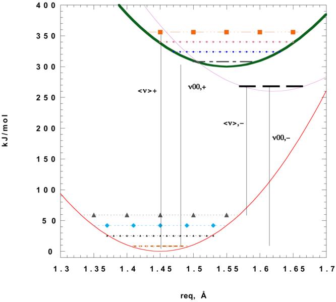
A representative Potential energy surface for a single vibrational mode. (Jablonski diagram). The values are realistic for a 1400 cm⁻¹ fundamental, with reduced mass of 6 Daltons. The excited state is shifted 0.1 Å for the absorption. The energies are also realistic, 0-0 excitation ∼ 399 nm, The resulting reduced phase (F-C) value, or Δx√(mω/ħ) is ∼ 1.6, which is large but not implausible. This value leads to the following F-C factors: 0.124, 0.2, 0.25, 0.216, 0.138, for excitation to the n′ = 0, 1, 2, 3, and 4 levels respectively. After dipolar relaxation, the surface is shifted further down and further out, 50kJ/mol and 0.065 Å respectively. These latter values are extraordinarily large for the sake of clarity (the fundamental is also assumed to decrease to 1350 cm⁻¹). The centroid up and down are indicated <ν>₊ (<ν>₋) respectively, and the 0-0 transitions ν_0-0 likewise.

Even if this assumption is mistaken, it is nonetheless possible that differences in e-m field work against (or by) the molecular framework in ‘up’ vs ‘down’ transitions are ‘intrinsic’ to the molecule itself, and would be a constant ‘remainder’ in comparisons with a variety of solvents. That assumption underlies the Lippert plot formalism, the intrinsic part is the ‘intercept’ of the plot, and does not (in the most fortunate cases) scale with the solvent function discussed below. This assumption, in turn, would seem questionable in cases where a fluorophore in one particular solvent displays this mirror image symmetry, yet where the symmetry is absent in a different solvent; for then the vibrational-solvent coupling in the latter solvent is sufficiently strong to destroy the mirror image symmetry observed in the first solvent, and because the excited state likely couples with different strength to this latter solvent than the ground state does, the two solvents may engender different F-C contributions. The logic of the case is that equality of Franck-Condon factors => equal displacement work => mirror-image symmetry(14,15). Thus, if a particular solvent system violates mirror image symmetry this implies the F-C factors are not comparable either. Further, as illustrated in Figure 1, if the solvent relaxation causes further equilibrium (or steady state nonequilibrium) displacement(16, 17) of a bond, relative to the initial state, then mirror image symmetry is voided, for the F-C factors aren't the same in the up vs. down transitions. We will consider this case in further detail in the discussion section.

As a practical matter, too, for fluorophores with fairly symmetrical absorption/emission band-shapes, it is much easier to measure their centroid wavelength, than it is to find their often-obscured 0-0 transition energies. Such considerations led us to utilize three different methods to measure the S.S.

Methods

Observational determination of S.S.

Method I) The definition of ‘center of mass frequency’ or centroid, is itself open to some debate -- one generally takes the center of mass of a spectrum to be <ν> = <E>/h = ∫ Ef(E)dE /(∫ f(E)dE) for the energy E, the frequency ν and ‘f’ the distribution function to be averaged. However, on could equally insist that in absorption

<ν>_up = ∫ ε(ν)dν /(∫ ε(ν)/ν dν) and in emission

<ν>_down = ∫ f(ν)/ν² dν /(∫ f(ν)/ν³ dν)) since these are the integrals relating the underlying oscillator strengths to the energy distribution of states in the respective excitons)(18). And this definition of centroid is what we employ in Method I, where we take these particular centroid difference-energies

Method II) is an attempt to find instead the 0-0 transition energy difference. We have fitted the experimental curves from Berlman(10) to functional forms involving sums of (at times, stretched) gaussians(19). We needed to do this to calculate the values for Method I in any case. With these in hand, underlying peaks can be taken as representative of the 0-0 transitions if we can distinguish the differing electronic transitions for indole, phenol and naphthalene labeled L_a and L_b, itself not always a straightforward task. The 0-0 absorption energies are also tabulated in Murov, Hug and Carmichael(20), which we give here in Table I, as is required for the implementation of the Thompson-Schweizer-Chandler algorithm. What we have done is take the 0-0 up transition energy from the literature, i.e. reference 20, and compared the bandwidths for our fitted bands to similar widths for bands fitted in absorption/emission in the various solvents, assuming the 0-0 L_a or L_b transitions have similar ‘narrow’ widths.

Table I.

steric and electronic parameters employed

for solvents
	aHS (Å)	α0 (10−24 cm3)	ε0	n	ρ*	ω0(kJ/mol)
Cyclohexane	5.2	11.0	2.02	1.427	0.79	951.5
Methanol	3.5	3.3	33	1.329	0.64	1047
Water	2.6	1.444	78	1.333	0.59	1218
AcNH2	4.05	5.67	22	1.428	0.48	931
for solutes
	asite	αI,0	αI,1	μgr (D)	μex	q(e0)), gr	q(e0)), exc	ωI (kJ/mol)
phenol	2.75	11.1	10.9	1.22	3.6	0.092	0.273	431np, 423p
indole	2.95	16	15.1	2.1	5.4	0.14	0.368	415np, 401p
α-NaphthNH2	3.20	19.5	18.5	1.15	3.4	0.072	0.216	348np, 325p

Legend – a_HS is the hard sphere diameter taken for the various solvents. α is the polarizability value we employ. ε₀ is the static dielectric constant, n the index of refraction (taken from the sodium D-line which may not be accurate for the wavelengths employed), and ρ* is the reduced number density of the solvent, given by: (mass density × N₀ /MW) × 10⁻²⁴ a_HS³. These values are all from Reference 32. a_site is the value we take for the solute effective radius (this is a purely assumed value). The dipole moment of the ground and excited states are μ_gr(μ_ex) are ‘arbitrary’ values for phenol and naphthylamine, but cf Ref 33, 34 for phenol, and Reference 35 for naphthylamine; the dipole moments of indole are from Reference 30. ω_I is the energy of the transition to the lowest vibrational level of the excited state in ‘polar’ (p) or in ‘nonpolar’ (np) solvents., and are taken from Ref. 20.

Method III – if in a given solvent there is no displacement of vibrational modes and no change in their frequencies, and no extra solvent stabilization of excited state charges, relative to the ground state, then the work difference between the centroid and the 0-0 up transition should be the same as that for the down transition (though opposite in sign), and there should be mirror image symmetry, as we argued above. The ‘intrinsic’ molecular distortion work is taken to be this difference. We assume that in cyclohexane the energy difference between the absorbance centroid and the 0-0 up-transition (which is usually well resolved) is equal to this intrinsic distortion work. Twice this value is subtracted from the energy difference found in our Method I, which should yield now the energy difference in excess of that required for just attaining the excited state, so all the work accomplished by the solvent, including further solvent-induced changes in vibrational modes is accounted for by this method (i.e. changes in centroid frequency due to changes in FC factor caused by the solvent coupling). We take cyclohexane as the reference solvent because it has what we expect to be the least coupling.

We also present the “Stokes' loss” values tabulated by Berlman(10). He defines S.S. as the wavenumber of symmetry' between the absorption and emission envelopes (the point at which there is as much of the absorption envelope mass on one side of this frequency as has the emission envelope on the other side) from which is subtracted the ‘centroid’ of the emission envelope. One sees that, should a given wavenumber have 50% of emission and 50% of the absorption on opposite sides, that the centroid of both bands are the same frequency and thus there is no S.S. On the other hand, assuming zero overlap of the absorption and emission bands, then the center of the void zone between them is the ‘symmetry’ wavenumber – and corresponds fairly with the arithmetic mean of the 0-0 up and down transitions. Then Berlman's S.S. is: (ν_0-0,+ + ν_0-0−)/2 − <ν>₋ which we would argue is (ν_0-0,+ + ν_0-0−)/2 − (ν_0-0−) + ν_dist = (ν_0-0,+ − ν_0-0−)/2 + ν_dist which corresponds to only half the ‘relaxation’ work of the solvent plus the distortion work against the molecular frame. It is not clear how useful this value is in general, although these fairly distinct objects may well be numerically comparable(21). We include both these methods, that of Berman, and that of Method I, here for comparison purposes, because they would be more typically employed in constructing Lippert plots, but are probably less relevant to the calculations we perform herein than the other two methods (II and III).

Calculation of Stokes' Shift : 1) The ‘classical’ formalisms

The classical theory of solvent shifts was developed many times, most completely early on by Ooshika(8) (cf. Amos and Burrows(6)), among others. The name ‘classical’ is used here because 1) there is nothing in the derivation thereof that specifically refers to quantum mechanics, and 2) the solvent is treated as a dielectric continuum, that is, as a structureless fluid, so that molecular effects of the solvent are also neglected.

The first version of the classical formalism is probably the most often derived form, and is quite popular:

$$\begin{array}{cc}\hfill & \mathit{Es}.s.\equiv \hslash c\Delta \varpi s.s.=2\{{\mu }_{\mathrm{f}}({\mu }_{\mathrm{f}}-{\mu }_{\mathrm{i}})∕{{\mathrm{a}}_0}^3\}[({\epsilon }_0-{\epsilon }_{\infty })∕({\epsilon }_0+2)-({n_{\mathit{sol}}}^2-1)∕({n_{\mathit{sol}}}^2+2)]+\hfill \\ \hfill & \{({{\mu }_{\mathrm{f}}}^2-{{\mu }_{\mathrm{i}}}^2)∕{{\mathrm{a}}_0}^3\}[({n_{\mathit{sol}}}^2-1)∕({n_{\mathit{sol}}}^2+2)]\hfill \end{array}$$ (1a)

where ε₀ is the static dielectric constant of the solvent and n_sol is its index of refraction. The μ_f (or μ_i) is the excited (ground) state static dipole moment.

The second version of the classical formalism we employ is(22):

$$\mathit{Es}.s.=2\{{({\mu }_{\mathrm{f}}-{\mu }_{\mathrm{i}})}^2∕{{\mathrm{a}}_0}^3\}[({\epsilon }_0-{\epsilon }_{\infty })∕({\epsilon }_0+2)-({n_{\mathit{sol}}}^2-1)∕({n_{sol}}^2+2)][(2{n_{\mathit{sol}}}^2+1)∕({n_{\mathit{sol}}}^2+2)]$$ (1b)

This version is one of the preferred choices of Koutek(22). In the derivation of these formulae, the F-C vibrational displacement is never taken into account. At best these formula, which refer to idealized static dipoles, must refer to the ‘slope’ of Lippert plots, i.e. the intrinsic vibrational terms must be carried over to the ‘intercept’. In its inverted form the classical formalism is most often employed in order to extract μ values. In order to test he formalism itself, we will work in the opposite direction.

The dielectric response theory encapsulated in equation (1) for the S.S. has certain other conceptual weaknesses. For one, it supposes the existence of a well-defined cavity for the solute-particle which excludes solvent, with the somewhat uncertain cavity radius ‘a₀’ yet the presence of explicit boundaries produces image charge-terms in any electric theory, the boundary terms involve the dielectric constant mismatch, which compromises either the concept of conserved charge or electric field continuity(23); and as we stated above, it treats the solvent outside the cavity as a dielectric continuum. Continuum theories and Reaction Field theories have entertained certain physical objections(24,25,26) and compared with explicit solvent models are, at least in Molecular Dynamics, generally employed only for long range electrostatics where the computational cost of including explicit interactions with particulate solvent molecules is prohibitive(26,27).

Ideally one would like to calculate the dipolar shift including specific solvent molecules at one or several specific sites on the solute, i.e. calculate the dielectric response as a function of time for each of the solvent molecules in the first solvation sphere individually, and model moreover as a separate ‘solvation shell’ the solvent molecules with which each of these particular solvent molecules interact, and to continue this process until the changes introduced are the same as one would obtain using bulk continuum dielectric models. This is a very large undertaking, especially as the dielectric response function at all frequencies has not been precisely modeled as yet for even one solvent, let alone for many different solvents. And it is unclear that anything less than a full quantum mechanical description for each of the possible nearest neighbor solvent molecules would suffice.

In a simplified model, instead, we would like to take advantage of the known properties of bulk solvents, without recourse to modeling specifically the properties of isolated solvent molecules. At the same time, we know that exclusion of solvent from cavities disrupts the solvent-solvent correlations that normally obtain, to a range well outside of the radius of the cavity. A fairly sophisticated statistical mechanical approach which still takes full advantage of the properties of the average solvent(28) was that developed in TSC and SCM(1,2,3). These are, then, the two such approaches: one specifically designed for polarizable, but nonpolar solvents, and the other adapted to dipolar solvents. In the event, we explicitly assume that these two kinds of effects are additive, hypothetically, it would be as if one starts with a hard sphere solvent, then adds a term that treats the solvent polarizability (like a perturbation treatment which converts the hard sphere-solvent to the Lennard-Jones solvent), which one then perturbs further to produce a dipolar, polarizable solvent. The TSC procedure is derived from an exact (within the mean spherical approximation29) treatment of hard sphere solvent. There is no assumption of ‘cavity’ diameter, only the reduced molecular density is employed. Thus we conceive that the contributions of solvent-impurity collision-induced polarization are included in the TSC model. A great deal of solvent relaxation occurs within the first few ps(30). In such time, given typical diffusion constants of ∼100 Ųns⁻¹, nearest-neighbor solvent molecules cannot easily exchange with bulk solvent. So we can reasonably conclude that this contribution refers to collision/dispersion-induced repolarizations by nearest neighbors only. These may also be unable to respond as reorienting dipoles during the first dozen ps of the excited state lifetime, particularly if they are neighbors of relatively charged heteroatoms. Thus, the second contribution (of the SCM model) we take to refer to the re-orienting solvent more characteristic of the second and larger solvation shells. First shell solvent would not, on this view, participate in density fluctuations typical of ‘bulk’ solvent. Thus, for the SCM method, we take the effective radius (inverse spatial frequency cut-off) to include the radius of the nearest neighbor solvent. Thus we justify our marriage of the two contributions.

We employ the following quantities (cf also Table I) which are relevant to ‘mean field renormalized polarizabilities(1) (the following defining equations are given by Thompson, et al.(1), or in their references):

$${\alpha }^{\prime }=-{\alpha }_0(\mathrm{B}\left(\omega \right)∕\mathrm{A}\left(\omega \right))[1-{(1-\mathrm{A}\left(\omega \right)∕{\alpha }_0{\mathrm{bB}}^2\left(\omega \right))}^{1∕2}]$$ (2a)

$$\mathrm{A}\left(\omega \right)=2{\alpha }_{0}b[{(\omega ∕{\omega }_0)}^2-1+2{\alpha }_0{\mathrm{E}}_{\infty }]$$ (2b)

$$\mathrm{B}\left(\omega \right)={(\omega ∕{\omega }_0)}^2-1+{\alpha }_{0}b$$ (2c)

$$a=4\pi \rho {\sigma }^{-3}{\mathrm{I}}_2\left(\rho {\sigma }^{-3}\right)\equiv 4\pi {\rho }^{\ast }{\mathrm{I}}_2\left({\rho }^{\ast }\right)$$ (2d)

$$b=(\rho ∕\pi ){\mathrm{I}}_3\left({\rho }^{\ast }\right)$$ (2e)

$${\mathrm{E}}_{\infty }\equiv a∕b$$ (2f)

$${\mathrm{I}}_2\left({\rho }^{\ast }\right)=[1-0.3618{\rho }^{\ast }-0.3205{\rho }^{{\ast }^2}+0.1078{\rho }^{\ast }3]∕{[1-0.5236{\rho }^{\ast }]}^2$$ (3a)

$${\mathrm{I}}_3\left({\rho }^{\ast }\right)=(1∕2.70797)[2.70797+1.68918{\rho }^{\ast }-0.31570{\rho }^{{\ast }^2}][1-0.59056{\rho }^{\ast }+0.20059{\rho }^{{\ast }^2}]$$ (3b)

The I₂ and I₃ integrals are given by Rushbrooke et al31) (and previous workers) and are adapted from Padë-Laplace approximants to the hard-sphere/Carnahan-Starling equation of state but including (I₂) the induced dipolar interaction tensor and (I₃) the induced Axilrod-Teller triple-dipole interaction. In the definitions (2), α₀ is the molecular mean polarizability of the solvent, ρ is the number density for the solvent, and σ is its effective diameter, thus ρ* is the reduced number density, ω is the energy of the light absorbed or emitted with ω_I the 0-0 up transition energy of the ‘impurity’ while ω₀ is the energy of the first excited state of the solvent. Every other term is only defined in context.

To implement their method, one finds first the renormalized energy E′(ω) = aα'(ω)/(1 + bα'(ω)) E′(ω) = aα′(ω) (1 + bα′(ω)); whence one determines

$$\mathfrak{R}\left(E^{\prime }\left(\omega \right)\right)=-(\mathrm{A}\left(\omega \right)∕\mathrm{B}\left(\omega \right))a{\alpha }_{0,\mathrm{I}}[1+b(\mathrm{A}\left(\omega \right)∕\mathrm{B}\left(\omega \right)){\alpha }_0(1-|f\left|\right)]∕{[1-b^2|{\alpha }^{\prime }\left(\omega \right)\left|\right]}^2$$ (4)

wherein :$\left|{\alpha }^{\prime }\left(\omega \right)\right|=|{\alpha }_0\mathrm{B}\left(\omega \right)∕\mathrm{A}\left(\omega \right)|\sqrt{1+\left|f\right|}$ and f = 1 − 2A(ω)/(α₀bB²(ω) where α_0,I is the ground state net polarizability of the fluorescent solute – the impurity.

The first contribution to Δν_SS is

$$0={{\omega }_{\mathrm{I}}}^2-{\omega }^2+2{\alpha }_{0,\mathrm{I}}{{\omega }_I}^2(\mathrm{A}\left(\omega \right)∕\mathrm{B}\left(\omega \right))a{\alpha }_0[1+\mathrm{b}(\mathrm{A}\left(\omega \right)∕\mathrm{B}\left(\omega \right)){\alpha }_0(1-|f\left|\right)]∕{[1-b^2|{\alpha }^{\prime }\left(\omega \right)\left|\right]}^2$$ (5a)

while the imaginary root of ω, or γ is such that:

$$\gamma =(a∕\omega ){\alpha }_{0,\mathrm{I}}\omega {{}_{\mathrm{I}}}^2(\mathrm{A}\left(\omega \right)∕\mathrm{B}\left(\omega \right))|f{|}^{1∕2}[1-2b(\mathrm{A}\left(\omega \right)∕\mathrm{B}\left(\omega \right)){\alpha }_0]∕[1-b^2|{\alpha }^{\prime }\left(\omega \right){|}^2(1+|f\left|\right)]$$ (5b)

Once we find γ, we must add the value γ² back to the value for the real root of ω² found above to determine the whole of the polarizability contribution to the new transition energy (i.e. √ (ω²_root + γ²)) which may be subtracted from the initial (0-0) transition energy for the solute, or ω_I given in the Table I. These transition values are what are listed in Table II. Since γ depends parametrically on ω, one has to iterate between the values till convergence, which is not in actual terms very time-consuming.

Table II.

solvent shifts for solutes:

TSC (kJ/mol)			Dipolar (kJ/mol)	shift(cm−1)	(from eq 1a)	(1b)	obs. shift I	II	III	obs. Shift (Berlman)
Phenol
	CH	425.7	−16.9	2090	310	279	4260	580	1230	2090
	MeOH	392.35	−23.5	5333	1545	2344	3970	600	950	2230
	H2O	399	−26.9	4569	1632	2500
	AcNH2	385	− 22.0	5268	1440	2130
-------------------------------
Indole
	CH	405.2	−21.2	2580	1216	434	4581	50(Lb) 2550(La)	2710	1930
	MeOH	352.6	−45.5	7803	5920	3650	6842†	3340(La)	4230	4100
	H2O	368.7	−52.4	7036	6249	3890	4950	2100	2340	2530
	AcNH2	350.9	−42.1	7663	5533	3310
-------------------------------
α-NaphthNH2
	CH	339.3	−7.4	1339	395	158	6175	2310	2770	2860
	MeOH	280.8	−15.6	4975	1982	1330	8900†	5700	5500	4120
	H2O	295	−17.9	3980	2090	1420
	AcNH2	280.5	−14.6	4914	1847	1210
-------------------------------

TSC is the solute transition energy calculated according to eq 5 (the Thompson-Schweizer-Chandler model1,2), ‘dipolar’ is the S.S. calculated from equ 7. Total shift is listed under “shift”. Berlman's values of S.S. are in reference 10. I, II, III refer to the methods used to calculate the S.S. (see text).

^†measurement is in solvent ethanol, not methanol.

The SCM theory(3) goes beyond the Mean Spherical Approximation(29) which was a basis for the above treatment. This treatment was a ‘time-dependent dielectric response’ consideration of Chandler's(5) previous gaussian field model of solvent. The solvent is considered to be a gaussian fluid. That is, a large times and distances it is structureless, but that the fluctuations near in time or space to a point have a gaussian structure. The cavity diameter ‘a’ is here considered for each pole of the excited state dipole, and as we argued above, we take the diameter of a single solvent molecule plus the radius of the solute that we suppose, somewhat arbitrarily, in Table II (under a_site). We reiterate that it enters the theory not as a boundary of the source's electrostatic potential, but as a momentum cutoff. The nearest neighbor solvents are included precisely because they do not, we assume, take part in the ordinary solvent-lattice-pseudovibrations (especially those solvent molecules nearest a pole). but do, we assume, mostly interact via instantaneous collisional and London-type forces on the solute(36). Under the ‘gaussian field’ framework, the solvation energy for a pole in a box cleared of solvent is:

$$\Delta {\mathrm{E}}_{\text{dipole - solvation}}=\int {\left(E\chi \right)}^{†}{\chi }^{-1}\left(\chi E\right){\mathrm{d}}^3\mathbf{r}$$ (6)

with ‘χ’ a time-dependent electric susceptibility tensor, and e the instantaneous electric field (a column vector). For two poles embedded in two boxes of width ‘a_site’ they obtain for the Laplace transformed ΔE(s) (‘s’ is the ‘rate’ variable obtained via the transform):

$$\Delta \mathrm{E}\left(\mathrm{s}\right)=({\mathrm{q}}^2∕{\mathrm{a}}_{\text{site}})\{1.088{(48∕\pi )}^{1∕3}[1-\epsilon {\left(\mathrm{s}\right)}^{-1}+12(6.066∕{\pi }^2)](1-\epsilon {\left(\mathrm{s}\right)}^{-1})∕[12\pi (2\epsilon \left(\mathrm{s}\right)+1)+3\epsilon \left(\mathrm{s}\right)-3]\}$$ (7a)

where ε(s) is ε_∞ + (ε₀ − ε_∞)/[1 + sτ_D] ε_∞ + (ε₀ − ε_∞)/[1 + sτ_D] we have already evaluated with respect to a cutoff frequency of k_c = {(2π/a_site)³/(4π/3)}^1/3 and we have so far an arbitrary value of the cutoff ‘a_Site’. For the steady state (or static) part as s—> 0, the SCM.(3) formula becomes (this expression is not explicitly given by SCM, but is promptly derived from the expression they do give):

$$\Delta \mathrm{E}=({\mathrm{q}}^2∕{\mathrm{a}}_{\text{site}})[2.7(1-{{\epsilon }_0}^{-1})+7.376(1-{{\epsilon }_0}^{-1})(78.4{\epsilon }_0+34.699)]$$ (7b)

Their rate formula, interestingly, generates a two-exponent decay for dielectric relaxation. Here ‘q’ is the embedded charge. What we are presented with, on the other hand, are dipoles in the ground and excited states; these have to be converted into ‘embedded charges’, thus, the input values of ‘q’ are taken to from the assumed dipole moments |μ| divided by the ‘distance’ (‘d’) between these poles. The values for these distances are obtained by the following considerations: In the ground state we imagine that the ground state polarizability is the effective Drude oscillator volume – i.e. the volume of a system whose harmonic oscillator potential reads U = 1/2 |μ|²/α = 1/2 q²(d)²/α. We now assume, somewhat arbitrarily, that α = 4π/3 (d/2)³ in order to find our ‘d’. Using the ‘isotropic’ value of the polarizability, this volume is taken to be spherical. For the excited state, we employ the well-known formula(37) for the polarizability α = ħ²e₀² /m_eΣf_i/ΔE_i² to write the polarizability of the first excited state as α₁ = α₀ − f₁e₀² /(m_e□²ω²) α₁ = α₀ − f₁e₀²/(m_elc² ω²) where f_i is the dipole strength of the i'th transition and ω = 2πν and ν is the mean frequency in wavenumbers of the first electronic transition. These α values are presented in the Table I. From them, we can now extract the dipole ‘distance’ of the first excited state and thence the excited state charges ‘q_ex’ as required for formula 7b. In the original SRM. formula, the electric pole is thought to exist in a vacuum cavity. Actually it is embedded in a dielectric (for us, an aromatic molecule) sphere inside a solvent of a different dielectric. So, to do some injury to the beauty of the original work, because of reintroducing boundary effects, we also add a ‘screening’ due to this dielectric mismatch^(38′) 3ε_solvent/(2ε_solvent + ε_solute) = η i.e. in the term at the front of formula 7b, q²/a_site, is replaced with q²/ηa; we use ε_solute = 2.5 for aromatics.

Results

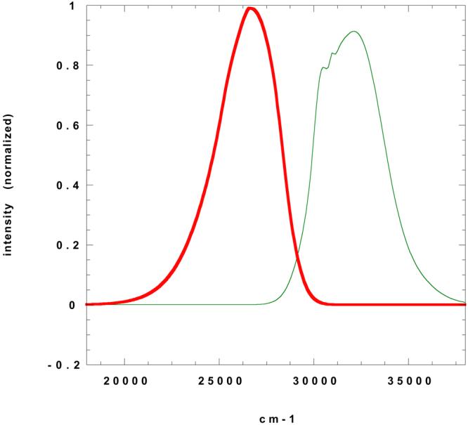
Figures 2 through 4 show the absorption and emission spectra of phenol, indole, and 1-aminonaphthalene (from Ref. 6) in cyclohexane and ethanol (in water for indole, and in methanol instead of ethanol for phenol). The absorbances must be scaled by 2300 for phenol in cyclohexane, 1900 for phenol in methanol, 5800 for indole, 5200 for aminonaphthalene in cyclohexane, and 6000 for aminonaphthalene in ethanol to yield molar extinction coefficients. Sloping' backgrounds from higher lying transitions have been subtracted by a cubic spline algorithm. But it is the spectral distribution which concerns us. The first two methods are applied directly to these spectra. However, for the Method II, involving 0-0 shifts, one must confront the presence of two different transitions, which complicate the assignment of the bands in indole and naphthylamine; the so-called L_a and L_b transitions. In both cases the preponderance of evidence is that L_a having the larger dipole, the excited state in polar solvent is mostly populated in the L_a state. So emission in these solvents is dominated by L_a. However L_b considerably overlaps the absorption envelope. And for the polar solvents, it is not easy to distinguish where the 0-0 L_a transition is in either absorption or emission. For indole it is known that the band at ∼ 288 nm is L_b. Murov et al(20) also give values for transition energies of the fluorescing state which are consensus (literature) values for the 0-0 absorption energies (and which we have employed in Table I). For emission, we utilize our fitting parameters to identify which bands have similar widths, the L_a emission origin being taken to have a similar width in emission in indole to that in absorption, and the L_b (taken to be narrower) likewise. Nevertheless in emission the L_a origin is hard to discern unambiguously. For example our fitting for indole in H₂0 we obtained in absorbance:

$$\begin{array}{cc}\hfill & 0.14\times \exp [-{(\varpi -{\varpi }_0)}^{1.55}∕100]\{\text{for}\varpi >{\varpi }_0\},+0.14\times \exp [-{({\varpi }_0-\varpi )}^{2.55}∕600]\{\text{for}\varpi <{\varpi }_0;{\varpi }_0=35880{\mathrm{cm}}^{-1}\}\hfill \\ \hfill & +0.5\times \exp [-{((\varpi -36300)∕1530)}^2]+0.33\times \exp [-{((\varpi -34965)∕295)}^2]\hfill \\ \hfill & +0.06\times \exp [-{(\varpi -{\varpi }_0)}^{2.45}∕380]\{\text{for}\varpi >{\varpi }_0\}+0.06\times \exp [-{({\varpi }_0-\varpi )}^{1.65}∕1030].\{\text{for}\varpi <{\varpi }_0;{\varpi }_0=37052{\mathrm{cm}}^{-1}\}\hfill \\ \hfill & +0.32\times \exp [-{((\varpi -37250)∕1420)}^2∕2]+0.10\times \exp [-{((\varpi -38400)∕1100)}^2∕2]\hfill \end{array}$$

; and in emission we found: :

$$\begin{array}{cc}\hfill & 0.975\times \exp [-{(({\varpi }_0-\varpi )∕2800)}^{1.8}]\{\text{for}\varpi <{\varpi }_0\}\hfill \\ \hfill & +0.975\times \exp [-{((\varpi -{\varpi }_0)∕2280)}^{1.9}].\{\text{for}\varpi >{\varpi }_0;{\varpi }_0=32350{\mathrm{cm}}^{-1}\}\hfill \\ \hfill & +0.047\times \exp [-{((\varpi -33780)∕1260)}^2]\hfill \end{array}$$

for ϖ in cm⁻¹; in comparison with literature values we concluded the narrow band at 34965 was the L_b origin in absorption, which led us to conclude that 35880 cm⁻¹ is the origin of L_a, which then leads, if 33780 cm⁻¹ is the L_a origin in emission, to the value for the 0-0 shift listed of 2100 cm⁻¹. For indole in ethanol we found an absorption band at 35530 cm⁻¹ which comports well with the L_a origin, but in emission there is no obvious ‘origin’ to be seen. We could instead use the value of the peak, which Callis(30) suggests is roughly 1500 cm⁻¹ lower in energy than the origin. Thus we arrive at the value in the table of 3340 cm⁻¹. For naphthylamine, one has a band fitted to 23294 cm⁻¹ in emission and 30500 in absorbance. But because it is so broad and unstructured, we subtracted again 1500 cm⁻¹ from this difference to obtain the value of the 0-0 transition listed in Table II. Thus, we consider these fittings not to be the most unambiguous source of 0-0 transition energies, since the 0-vibrational origin in emission may be very weak, and unresolved because of extensive spectral broadening. The larger solvent dipolar coupling that takes place, the more broadened the spectrum should also be (see below). Method II, then, unless backed up by other data, or by other kinds of spectroscopy, is not able to reliably recover the 0-0 transition energies. Given these caveats, our expectation is that these energies should be closer to the values from the classical formulae, which are purely dipolar terms, while the values including vibrational contributions, i.e. centroid differences, would include both dipolar and polarizability contributions. And so those values from Method III should comport better with our ‘new’ formulas.

Figure 2a.

absorption and emission of phenol in cyclohexane. 2b) absorption and emission of phenol in methanol. Adapted from Berlman. (Ref.14)

Figure 4a.

Absorption and emission of 1-aminonaphthalene in cyclohexane; 4b) absorption and emission of 1-aminonapthalene in ethanol. (Ref 14)

In general, if we focus on the predictions vs. the results of Method II and III, we see that, indeed Method II is closer to the classical results (from eq 1a and 1b) than Method III. Comparing between the classical formalisms, as Koutek(22) also found, his equation (1b) is closer to the value of S.S. It is also interesting that there is rough agreement between Method II and III and indeed with Berlman's method. Our Method I seems to exaggerate the total shift. It is likely to be subject to overemphasizing the effect of near-lying absorption transitions which, although they appear in absorbance at energies slightly above the transition to the emitting species, may not contribute to fluorescence; these bands will cause the centroid difference to be exaggerated. Also the centroid will necessarily be moved to longer wavelengths; however the subtraction of the 0-0 absorbance in cyclohexane seems to compensate for these effects and we obtain (in Method III) quite reasonable values for the S.S.

In Table II, our predictions are often too large. However in many cases they are better than the classical formalism. Especially interesting are the results in MeOH vs H₂O for indole. In methanol we unambiguously predict a larger Stokes shift of indole than in water. This is because the polarizability in this case has a larger effect than in some other solutes, when compared with the pure dipolar part (which is usually similar to the classical values). Methanol is expected by the TSC + SCM algorithm to cause a larger S.S. for indole than water is, but the classical formulae result in the opposite conclusion. Yet, regardless of the particular method employed, the S.S. from methanol is unambiguously greater than from water for indole. Here then, there is clear evidence of an effect that contradicts the classical formulae, yet is distinctly predicted by the new formulas. This new algorithm we employ herein also appears particularly effective for the naphthylamine data. On the whole, then, the new methodology appears to be an improvement over the classical formalism.

Discussion

Role of cavity parameter and dielectric constant chosen

For the exact values calculated by either formula, much depends on the choice of the solute radius ‘a’ parameter. Some authors(39) enlarge this radius because the various formulae such as (1a) or (1b) seem also to exaggerate the dipole moment obtained from using more molecularly ‘reasonable’ values. There is, however, no good theoretical justification for choosing values of ‘a’ which do not comport with molecular models, based as they are on X-ray scattering and other physical data. Another possibility is that the ‘static’ dielectric constant should actually be taken to be closer to the high frequency (but not yet the optical) dielectric constant(40), ε_∞ which would make the predicted shifts smaller with the same given ‘a’ values. Physical justification for this move is better, in asmuchas the nearest neighbor solvents are not surrounded by bulk-like solvent molecules, and the diffusion time for one solvent diameter is ∼ tens of GHz, within which time regime, its response is closer to ε_∞. Using a value of ε_∞ of ∼ 4.6 for water results in a change equivalent to a change from ‘a’ = 3.0 to ‘a’ = 4.0 Å, which has been used to ‘correct’ indole dipole moments obtained from Lippert plots(39). However, the time scale of the fluorescent state itself certainly suggests that ε₀ should be used. The formula employed for the rate dependent dielectric by SCM, or ε_∞ + (ε₀ − ε_∞)/[1 + sτ_D] is derived from a Laplace transform of the usual expression which is more traditionally Fourier transformed to yield the real and imaginary parts of the frequency dependent dielectric constant(38). Phenomenologically, if we envision two steps in the dielectric relaxation process: P₀—>P₁—>P₂ with characteristic rates k₁ and k₂, while all fluorescent ‘species’ have the same single decay constant k, we obtain the following probabilities pf each species per unit time:

$$P_0\left(t\right)=P_0\left(0\right)e^{-(k_1+k)t}$$ (8a)

$$P_1\left(t\right)=[k_1∕(k_2-k_1)]P_0\left(0\right)\{e^{-(k_1+k)t}-e^{-(k_2+k)t}\}$$ (8b)

$$P_2\left(t\right)=[k_2{k}_1∕(k_2-k_1)]P_0\left(0\right)\{e^{-(k_2+k)t}∕k_2-e^{-(k_1+k)t}∕k_1+[1∕k_1-1∕k_2]e^{-\mathit{kt}}\}$$ (8c)

If one differentiates each above term by ‘t’ this can be substituted for ‘s’ in the above expression for the rate-dependent dielectric constant to give, again phenomenologically, an estimate for the ‘ε(s)’ and hence the dipolar shift expected for each ‘P’. Time-resolved emission spectra which reflect the response of fluorophores to slow dipolar relaxations have been objects of study for some time(9). For many fluorescent states the fluorescent decay rates ‘k’ are much longer than any dielectric relaxation rates k₁ or k₂, and so ε₀ is appropriate. In viscous solvents it is possible that one or another fluorescent P species will be shifted differentially because the decay rates are now comparable to dielectric relaxation components. This ‘dynamical S.S.’ phenomenology could conceivably be manifest even if there were just one fluorescing electronic state, i.e. that the P's in (8) differ only by ‘degree of advancement of solvent relaxation’, not in any other way (cf. also Ref's 16, 17, and 41).

Alternative approaches

As we have argued, the 0-0 energy difference depends mostly on solvent dipolar relaxation. However some vibrational contribution, i.e. that due to dispersion-related changes in equilibrium bond length, is likely included in the TSC methodology. The work of Herman and Berne(42) provides a justification for the inclusion of the TSC-modelled contribution.

Herman and Berne(42) considered that the effective Lennard-Jones (L-J) interaction with solvent must be functionally dependent on the instantaneous bond length, the L-J perturbation then effectively skews even the ground state distribution of frequencies well away from the gaussian when any such bond-length L-J coupling is introduced. It also shifts the set of frequencies to the red at low solvent densities (attractive zone) and to the blue at high densities. They were able to predict that if the L-J coupling to the solvent is larger in the excited state, there is a red shift in both absorption and emission, and contrariwise if the L-J coupling is smaller. Whereas without any change in coupling strength, but merely in size, a red shift in emission and a blue shift in absorption is observed if the excited state is ‘larger’. They formalized their molecular dynamics based spectral results within the semi-quantitative model:

$$\Delta h\nu =\hslash ({\mathrm{n}}_{\mathrm{exc}}{\omega }_{\mathit{exc}}-\mathrm{n}{\omega }_{\mathrm{gr}})+{\rho }_{\mathrm{sol}}\int {\mathrm{d}}^3\mathbf{R}({\mathrm{g}}_{\mathrm{exc}}\left(\mathbf{R}\right){\mathrm{V}}_{\mathrm{S}-\mathrm{exc}}\left(\mathbf{R}\right)-{\mathrm{g}}_{\mathrm{gr}}\left(\mathbf{R}\right){\mathrm{V}}_{\mathrm{S}-\mathrm{gr}}\left(\mathbf{R}\right))$$ (9)

where the difference between average absorption and emission energies is Δ hν, the intrinsic vibrational-only difference (due to different vibrational energy wells in the ground state, vs. the excited state) is ħ(n_exω_ex − n_grω_gr) while the solvent induced S.S. is given by the next term. That term involves the difference in solvent position-dependent solute-solvent interaction V_s and in the solute-solvent 3-d pair correlation functions of the ground and excited states, the g(R) (see Figure 5). The integral is taken over all the solute-(in actuality a different integral should be taken for each solute site)-solvent displacements R. The vibration of the solute is modeled on a Morse oscillator, with parameters of r_eq the ‘zero’ of the Morse potential in vacuo and the dissociation energy in vacuo or D₀. The solvent can bring about S.S. by two means: 1) changing the effective D_eff from the value D₀ by changing the effective attractive field of the vibration, and 2) changing the effective equilibrium bond length r_m. The latter effect will change the Franck-Condon factors from the result in vacuo. This latter effect of the solvent in configuration X_sol displacing the effective equilibrium bond-length can be quantitatively given by(42)

$$\begin{array}{cc}\hfill & {\partial }_{\mathrm{rm}}∕\partial X_{\mathrm{sol}}=-({\partial }^2\mathrm{V}∕\partial X_{\mathrm{sol}}\partial \mathrm{r})/{\partial }^2\mathrm{V}∕\partial {\mathrm{r}}^2=\hfill \\ \hfill & -(1∕a)\partial ∕\partial X_{\mathrm{sol}}(1-\exp (-a(\mathrm{r}-{\mathrm{r}}_{\mathrm{eq}}))∕[2\times \exp (-a(\mathrm{r}-{\mathrm{r}}_{\mathrm{eq}}))-1])\hfill \end{array}$$ (10)

where V is the actual potential of the vibration in the presence of the solvent. The change in equilibrium position of a given vibrational mode is the ratio of the solvent perturbation of the instantaneous force on the mode to the mode force constant. Thus, if one imagines a change in solvent or solvent configuration δX that decreases the restoring-force on a bond, keeping the force constant nearly the same, it must do so by moving the r_eq to larger values, i.e. weakening the bond. If the solvent provides an attractive potential to the bond, as is usually assumed for solvent relaxation, then the bond will move outward, and consequently (see Figure 1) the F-C factors will be larger, and the most likely vibrational peaks will shift to lower energies in emission, so the emission envelope will move further red but will also (since the F-C factors are larger) be broader. Not for every possible change in bond polarization is a solvent dipolar response expected to be attractive; on the other hand, however, the ‘polarization’ response (i.e. that due to a term ∼ αE²) is attractive as long as the local field is stronger in the excited than in the ground state..

Figure 5.

The radial distribution factor for water at 20°C, and a perturbed g-factor for water due to relaxation of dipoles about a new source dipole. The perturbation was accomplished by application of the formula: g_new(r) =(g(r)⁰ − 1)exp(−ρ_sol∫ΔV(r)g(r)⁰ /kT d³r) + 1.00 where for ΔV(r) = we use a model of Langevin dipoles for water. Defining b = μ_solE(r) /kT with E(r) = u_rμ_I /r³ (1 − 3u_rcos²θ cos²ϕ) and u_r is in the Langevin approximation(33) equal to: (1/3)b − (1/45)b³ +(2/945)b⁵ − (2/9450)b⁷ ….and we use 1.84 D for μ_σ, 3.5 D. for μ_I in the excited state and μ_I = 0.75 D in the ground state (as in the body of the paper ρ_sol is the solvent number density -- or .0335/ų for water). The change occurring when we add a ‘polarizability term’ as well to ΔV, equal to 1/2 α ΔE(r)² is also included, with α = 1.444 ų. The initial g(r) for water about a ground state dipole could be similar to g(r)⁰ and the ‘equilibrium’ g(r) for the excited state would be the perturbed g(r).

Considerations along the lines introduced by the results of Herman and Berne can be employed to develop an alternative and novel approach to the vibrational origin contribution to Stokes' shift caused by solvent dispersion/collisional processes. These ideas are presented more fully in Appendix A.

Currently time dependent density functional formalism(13) is one of the methods of choice for determining low energy spectra of molecules. Essentially the problem is to calculate the momentary dipole moment μ(t) of the molecule given a ground state electron density distribution (and the so-called Kohn Shams density(43), which is roughly a set of N electron densities with either ‘0’ or ‘1’ the occupation number of orthonormal natural orbitals, each of which are solutions for the Fock operator with the exchange-correlation potential as a correction); The system is allowed to respond to the slowly varying field -- the response of this system in time to a small applied electric field can be written in such a way as is reminiscent of the approaches we have used so far: If we let a dipole susceptibility be written as(13, 44):

$$\begin{array}{cc}\hfill & {\chi }_{\mathrm{KS}}(\mathbf{r},{\mathbf{r}}^{\prime },\omega )=\underset{\mathrm{ij}}{\Sigma }{\phi }_{\mathrm{i}}{\left(\mathbf{r}\right)}^{\ast }{\phi }_{\mathrm{j}}\left({\mathbf{r}}^{\prime }\right)\rangle \mathbf{r}\langle {\phi }_{\mathrm{j}}{\left({\mathbf{r}}^{\prime }\right)}^{\ast }{\phi }_{\mathrm{i}}\left(\mathbf{r}\right)\mid {\mathbf{r}}^{\prime }/(\omega -{\omega }_{\mathit{ij}}+\mathrm{i}{\delta }_{+})-\hfill \\ \hfill & \underset{\mathrm{ij}}{\Sigma }{\phi }_{\mathrm{i}}{\left(\mathbf{r}\right)}^{\ast }{\phi }_{\mathrm{j}}\left({\mathbf{r}}^{\prime }\right)\rangle {\mathbf{r}}^{\prime }\langle {\phi }_{\mathrm{j}}{\left({\mathbf{r}}^{\prime }\right)}^{\ast }{\phi }_{\mathrm{i}}\left(\mathbf{r}\right)\mid \mathbf{r}/(\omega +{\omega }_{\mathit{ij}}-\mathrm{i}{\delta }_{+})\hfill \end{array}$$ (11)

where ω_ij is the difference in energies of the Kohn-Shams orbitals ‘i’ and ‘j’, H_F-xc φ_i and H_F-xcφ_j. (with H_F-xc being the Fock Hamiltonian with a exchange-correlation potential in addition). We have the square of the transition densities for the i–>j transition which is multiplied by the operators for the dummy space vectors r and r′ (the densities are integrated over all electron coordinates but one, the r or r′ to which they are associated). There is a close similarity of the above ‘susceptibility’ propagator with the polarization propagator given by Jorgenson(44).

Then one may write:

$$\begin{array}{cc}\hfill \chi & (\mathbf{r},{\mathbf{r}}^{\prime },\omega )={\chi }_{\mathrm{KS}}(\mathbf{r},{\mathbf{r}}^{\prime },\omega )+\hfill \\ \hfill & \int {\mathrm{d}}^3{\mathbf{r}}^{‴}\int {\mathrm{d}}^3{\mathbf{r}}^{″}{\chi }_{\mathrm{KS}}(\mathbf{r},{\mathbf{r}}^{″},\omega )<\underset{\mathrm{ij}}{\Sigma }{\phi }_{\mathrm{i}}\left({\mathbf{r}}^{‴}\right)\left|\{[e_0∕|{\mathbf{r}}^{‴}-{\mathbf{r}}^{″}|+{\mathrm{v}}_{\mathrm{ext}}]∕{\omega }_{\mathrm{ij}}\}\right|{\phi }_j\left({\mathbf{r}}^{‴}\right)>\chi ({\mathbf{r}}^{\prime },{\mathbf{r}}^{‴},\omega )\hfill \end{array}$$ (12)

as an integral equation for the dipole-susceptibility χ. The above equation can be thought of as the application of a quasiunitary transformation to ‘rotate’ an operator (or propagator) in one orthonormal basis to a new orthonormal basis corresponding to the solution in hand. Then (after convergence and Fourier inversion):

$$\mu \left(\mathrm{t}\right)\int {\mathrm{dt}}^{\prime }\int {\mathrm{d}}^3\mathbf{r}\int {\mathrm{d}}^3{\mathbf{r}}^{\prime }\chi (\mathbf{r},{\mathbf{r}}^{\prime },\mathrm{t}-{\mathrm{t}}^{\prime })E\left(\mathrm{t}\right)$$ (13)

which ought to remind one of μ(t) = α(□) • E (t) μ(t) = α(t) • E(t) which has the same physical content.

The poles of the response function χ (or α) are at the excitation energies and the residues there are the oscillator strengths for the transitions. An adaptation of this kind of TD-DFT program to the calculation of S.S. is possible with an extension of the external potential to include solvent interaction (in the nuclear electronic potential)(45, 46). Unfortunately, unless one then extends into a consideration of the electronic density of the solvent molecules themselves, one must generally have recourse again to approximate expressions for solvent-solute effects that physically similar to the approaches one has already heretofore employed. Thus, in one class of TD-DFT results authors(47, 48) have had recourse to a polarizable continuum approach. Here the ‘cavity’ is defined as essentially a solvent-accessible contour of the impurity, bounding which is a surface with a set of induced charges distributed about the solute given by means of the solute's (the source) electrostatic potential and the dielectric mismatch function as a local susceptibility (i.e. q_i (r) = f (ε)V_impurity(r) where q_i is the charge at a small surface element located at r). The solvent is however, not explicitly modeled, and at least for Molecular Dynamics simulations of solutions, as we mentioned above, a dielectric continuum is not considered an adequate approximation. It seems a priori doubtful that it will be adequate for ab initio methods for a considerable future. The continuum approach is, arguably, reasonably accurate in the same approximate sense that the classical methods of S.S. analysis (or Born solvation calculations, for another example25) are reasonably accurate, and thus, while not perfectly satisfactory, are nonetheless still useful. If one does the (more difficult) former modelling, essentially a supermolecule approach, one recovers most solvent effects as due to collisional+ dispersion effects from the exchange-correlation effect of solvent electrons on solute electrons, in other words the sort of effects to which the TSC treatment applies. In a way, this provides further justification for our treatment of these effects as due to nearest-neighbor, collisonal/dispersion effects. As an instance of explicit solvent calculations, Neugebauer et al(45,46). have treated the fluorophore-solvent system with a constrained TD-DFT method in their solvatochromism calculations. There, the authors used MD calculations to arrive at a set of explicit solvent configurations which were then subjected to TD-DFT calculations. These authors did indeed treat a few selected solvent molecules within the supermolecule approach, specifically including exchange-correlation effects with nearest neighbor molecules. The majority of explicit solvent molecules contributes via the electron density and nuclear charge terms alone, supplemented, however, by the quantum mechanical effect of confinement(45, 46) – that is one extra term in the v_ext expresses the difference in the kinetic energy density-functional of the whole system minus that of its separate ‘frozen’ parts, and thus is the response of the impurity electrons to confinement by explicit solvent electron density. Perhaps the most useful result out of TDDFT formalism is that vibrational displacements in the excited state are automatically included, so that the vibrational contribution to the centroid shift, as is the case with other ab initio methods, can be obtained. How these vibrational shifts are further affected by solvent interactions, is, as we see, still problematic(17).

There is another modern alternative treatment of the dielectric/dipolar part of the response, that is, the 0-0 shifts beyond the (as we assume) dispersion-related vibrational (or F-C) contributions., we would suggest. A proposal for a ‘field theoretic’ treatment which in some ways unifies the two approaches taken in this paper for the purely dipolar effects, both the gaussian fluid model, and the ‘classical’ models, is presented in Appendix C. Field theoretic models have been employed for the statistical mechanics of phase transitions.(49) The problem of dipolar relaxation in the liquid state might be compared with the general problem of the decay of ‘order’ in a liquid (see Figure 5): in the 1^st solvation shell we have what is essentially a quasilattice. By the 3rd solvation shell, we have essentially bulk, isotropic liquid. Between the one point and the other, the ‘order parameter’ characterizing the nearby pseudolattice has decayed to zero, and the symmetry group has become SO₃, while long range longitudinal phonons rather than transverse (librational?) phonons are propagated through the bulk phase. It is precisely in this region where we divide the contribution between the TSC and SCM models, while in Appendix C we seek to at least begin to model this ‘phase transition’-like behavior.

The invertibility of the classical approaches is probably the reason for their popularity. TSC and SCM, or their marriage as attempted in this report, are arguably less easily invertible. However, one could systematically and algorithmically ‘try’ various input μ's (and ‘q’s) and recover best fits. Techniques requiring detailed molecular dynamics simulations are less ‘invertible’ since they are more computationally intensive. Ab initio methods like TD-DFT are not really ‘invertible’, but since much more information is in principle obtained via them than can be got from any number of experimental observations, they should, if reliable, yield results in agreement with the best spectroscopic analyses, including TSC plus SCM.

Conclusion

we have examined two recent approaches to calculating S.S. from molecular parameters. These are comparable and in some cases superior to the older methods. They cannot, however, be as easily inverted, as in Lippert plots, where S.S. is plotted against a simple solvent ‘function’ and whose linear slopes are related to the difference of excited from grounds state dipole moments, without more extensive computational effort. Other alternatives are perhaps on the horizon, but it seems that for the time being, the ‘classical’ formalism, if judiciously applied, especially in the form of equ. 1b will still be with us for some time.

Figure 3a.

Absorption and emission of indole in cyclohexane; 3b) absorption and emission of indole in ethanol; 3c) absorption and emission of indole in water. (Ref.14)

Appendix A

In the approach here for vibrational equilibrium shifts induced by solvent coupling we invoke a simple Harmonic Oscillator instead of Herman and Berne's(42) Morse Oscillator. But the simple model we adduce here involves the simultaneous solution of the following equations:

$$\Delta {\mathrm{V}}_{\text{bond}}=1∕2\mathrm{M}{\omega }^2{\left(\delta {\mathrm{r}}_{\mathrm{eq}}\right)}^2$$ (A1a)

with ‘M’ the reduced mass of a bond, and ω the vibration frequency times 2π. δr_e the change in equilibrium bond length.

$$\Delta {\mathrm{V}}_{\text{solvent}}=\mathrm{g}{\left(\mathbf{R}\right)}^{-1}\mathrm{dg}\left(\mathbf{R}\right)∕\mathrm{dR}\mathrm{kT}\delta (\mathbf{R}-{\mathbf{r}}_{\mathrm{eq}})$$ (A1b)

R is the vector from the solute site to the solvent site. In a sense the value of δ(R – r_e) is ill-defined except for the case of a linear bond-solvent arrangement: A—B- - - -Solv., yet we know that a change in r_eq may also lead to a change in R, so that δ(R – r_eq) asks for this change in R dependent on (but in excess of) δr_eq This is the change in potential of mean force for the solvent due to changes in bonding in the solute.

$$\Delta {\mathrm{V}}_{\text{solvent - solute}}=-(6{\mathrm{C}}_6∕{\mathrm{R}}^7)\delta \left(\mathrm{R}\right)$$ (A1c)

the dispersion contribution from solvent nearest neighbors. C₆ is the dispersion coefficient for the 1/R⁶ potential.

$$\Delta {\mathrm{V}}_{\text{bond}}-\Delta {\mathrm{V}}_{\text{exch - corr}\left(\text{bond}\right)}=‘\text{excess distortion work in up}\left(\text{down}\right)\text{mapping}’$$ (A1d)

Assume that

$$\begin{array}{cc}\hfill & -\Delta {\mathrm{V}}_{\text{exch - corr}\left(\text{bond}\right)\mathrm{i}}={\chi }_{\text{bond},\mathrm{i}}\Delta \mathrm{q}{}_{\text{bond},\mathrm{i}}=\chi {}_{\text{bond},\mathrm{i}}\xi {}_{\text{bond},\mathrm{i}}\mu {}_{\text{bond},\mathrm{i}}∕{\mathrm{r}}_{\mathrm{eq},\mathrm{i}}=\hfill \\ \hfill & {\chi }_{\text{bond},\mathrm{i}}\Delta \mu {}_{\text{bond},\mathrm{i}}∕{\mathrm{r}}_{\mathrm{eq}},{}_{\mathrm{i}}-\chi {}_{\text{bond},\mathrm{i}}\mu {}_{\text{bond},\mathrm{i}}\delta {\mathrm{r}}_{\mathrm{eq},\mathrm{i}}∕{\mathrm{r}}_{\mathrm{eq},\mathrm{i}}\hfill \end{array}$$ (A2)

The basis for this equation is from the following considerations: each ‘bond’ in the system is taken to be repolarized by the excitation map of the electronic coordinates into the excited-state coordinates (the nuclear mapping defines the external potential which is taken to be unique to the state, all the other terms, the electron energy with the field of the other electrons, the correlation and exchange energies, depend parametrically on the nuclear position), this repolarization energy is (∂E_bond/∂n)δn_bond, or the derivative of the bond energy with respect to electron occupancy times the change in electron occupancy. (∂E_bond/∂n) is the ‘electronegativity’, and as per Parr and Wang(43) we can call the local aspect of it the bond electronegativity. If each bond has a given dipole moment μ_{i, bond} which is r_eq_i ‘q_i’ being the effective charge at the nuclear position (above the screened charge at the nuclei, in other words, it is the bond ‘charge’). But the change in dipole moment for each bond is Δμ_bond = Δ(r_eq_i) = r_eδq_i + q_iδr_e. Now, δq_i = q_iξ_I where ξ is the fraction of the initial charge q_i by which the bond-charge is altered (it can be positive or negative), while the q_i = μ_i/r_e. . The term involving the change in bond length alone is subtracted from the total change in dipole moment Δμ. We make the assumption that the vector sum over all bonds of Σ_i Δμ_i,bond would equal the total change in dipole moment for the molecule between the two states. One can assume the minimal vector sum of all such “bond-vectors changes” to equal the vector difference of the excited state – ground state dipole.

We assume now that the sum of excess distortion work equals the ‘dispersion/solvation’ work contribution, the excess of the F-C- factors beyond the minimum necessary to establish the charge distribution of the excited state. Then we arrive at this formula from which we can determine δr_e and hence the altered Franck-Condon factors for the excited state.

$$\begin{array}{cc}\hfill 1∕2\mathrm{M}{\omega }^2& {\left(\delta {\mathrm{r}}_{\mathrm{eq}}\right)}^2+\delta {\mathrm{r}}_{\mathrm{eq}}[{\chi }_{\text{bond}}{\mu }_{\text{bond}}∕{{\mathrm{r}}_{\mathrm{eq}}}^2-(6{\mathrm{C}}_6∕{\mathrm{R}}^7)\Psi ∕\{\Psi -(6{\mathrm{C}}_6∕{\mathrm{R}}^7)\}]-{\chi }_{\text{bond}}\Delta {\mu }_{\text{bond}}∕{\mathrm{r}}_{\mathrm{eq}}=0\hfill \\ \hfill & ;\text{with}\Psi =\mathrm{kT}g{\left(\mathrm{R}\right)}^{-1}\mathrm{dg}\left(\mathrm{R}\right)∕\mathrm{dR}\hfill \end{array}$$ (A3)

The quadratic can be solved for δr_eq from which we can write e.g. the Morse Oscillator Franck-Condon factor (M.O. FCF -- see Appendix B), assuming only that dispersion forces are responsible for the ‘excess’ energy of the distortion work, the FCF above and beyond the minimum necessary to map into the vacuum excited state. Since this solvent-dispersion induced FCF is evident in absorption, even before the solvent dielectric response can take hold (e.g. in comparison of other solvents w.r.t cyclohexane), it is independent of dielectric relaxation contributions (the further shifting of the vibrational origin - cf Figure 1)

Appendix B

We supply here the Franck-Condon factors for displaced Morse oscillators.

We write the 0′th M.O. as displaced, thus avoiding writing the Laguerre polynomials for a displaced oscillator: 2K = 1/f ; f = the anharmonicity factor, or K = 2D₀/ħω

$$\mathrm{V}\left(\mathrm{r}\right)={\mathrm{D}}_0[\exp (-2a(\mathrm{r}-{\mathrm{r}}_{\mathrm{eq}}))-2\exp (-a(\mathrm{r}-{\mathrm{r}}_{\mathrm{eq}}))]\equiv {\mathrm{D}}_0[\exp (-2u)-2\exp (-u)]$$ (B1)

$$\begin{array}{cc}\hfill & {\left(0\prime |{\mathbf{n}}_0\right)}_{\mathrm{M}.\mathrm{O}}=\hfill \\ \hfill & \left(\exp [-{\mathrm{Ke}}^{-u}{\mathrm{e}}^{-\Delta }]{\left\{\left(2{\mathrm{Ke}}^{-u}\right)\right\}}^{(\mathrm{K}-1∕2)}{\left(2{\mathrm{Ke}}^{-\Delta }\right)}^{K-1∕2}|\exp (-{\mathrm{Ke}}^{-u}){\left(2{\mathrm{Ke}}^{-u}\right)}^{\mathrm{K}-\mathrm{n}-1∕2}\right)\hfill \\ \hfill & {\left({\mathrm{e}}^{-\Delta }\right)}^{(\mathrm{k}-1∕2)}\left({\mathbf{n}}_0|\exp (-\mathrm{K}({\mathrm{e}}^{-\Delta }-1){\mathrm{e}}^{-u})|0_0\right)\hfill \end{array}$$ (B2)

we now employ the matrix elements published(50) for (0|exp(−λx)|n), namely:

$$\left(\mathbf{n}\right|\exp (-\lambda \chi )\left|0\right)={(-1)}^{\mathrm{n}}{\{(2\mathrm{K}-2\mathrm{n}-1)(2\mathrm{K}-1)∕[\mathrm{n}!\Gamma \left(2\mathrm{K}\right)\Gamma (2\mathrm{K}-n)]\}}^{1∕2}[\Gamma (n+\lambda )\Gamma (2\mathrm{K}+\lambda -\mathrm{n}-1)∕\Gamma \left(\lambda \right)]$$ (B3)

now we define λ₁ as K(e^−Δ − 1) and we expand the form exp(−K(e^−Δ − 1)e^−ax as a Taylor series in ‘x’, whereby we recover the approximate form

$$\exp (-{\lambda }_1)\{\exp \left({\lambda }_{1}a\mathrm{x}\right)-{\lambda }_1[\exp (-a\mathrm{x})-1+a\mathrm{x}+\dots ]\}$$ (B4)

This expansion is accurate up to terms in a³x³. One then uses expression (B3) with “λ” = λ1 for the first term in (B4).

The term in exp(−ax) can be evaluated directly with the same expression (B3) using λ = 1. The term in (ax) can be evaluated via the expressions given(51, or less accurately by taking logarithms of (B3) with λ = −1 (and remembering that Γ(n+λ)= (n+λ−1)(n+λ−2)(n+λ−3)… λΓ(λ); thus Γ(λ) as λ—>0 cancels in (B3)

Appendix C

We seek an analogy with the ‘polaron’ model of a free electron in a medium, though we now consider a purely dipolar ‘quasiparticle’ in a medium – a ‘dipolaron’ theory(52), namely a quantum field theory, possibly transcribed into path integral language, describing a bosonic dipole in the solvent and its mass (which leads to its short-ranged behavior) characterized by the dipolar medium's response to it, which response yields a screening factor. A massive vector boson is a known model from Quantum Field Theory(53,54). It also, except for the‘time’ term, resembles the Gaussian approximation to the Landau-Ginzburg model for order parameters in phase transitions(49). Indeed the alignment of solvent dipoles about a nascent impurity dipole is very like a phase transition: the fact that the order only extends to relatively short distances is the responsibility of the ‘mass’ term. We expect, as with the massive boson model, and as in the Debye model of solution electrostatics, to obtain a function of the dipole-order parameter to be of the form ∼ κ(μ_I/r) exp(−κr) . If we take the Klein Gordon model as a starting point(53,54),

$${\partial }_{\mu }{\partial }^{\mu }\varphi =-(m^2{c}^2∕{\hslash }^2)\varphi =(-1∕c^2){\mathrm{d}}^2\varphi ∕{\mathrm{dt}}^2+{\nabla }^2\varphi$$ (C1)

where ϕ is our ‘pseudoparticle’ wavefunction which we wish to roughly characterize as an ‘order parameter’ for the system. One possible solution for ϕ is identical with the solution for the vector potential of a radiating dipole (55) together with the electrostatic potential of the dipole, or the four-vector (Φ, A_r) = ([μ • r /r³], iωμ/r exp(−i(ωt+ k₀•r)), where the characteristic energy of the ‘lattice’ vibration is hω. and μ; is the source dipole moment; to the A_r term we can multiply an additional term exp(−κr) (the ω can also be modified to ω + 2 πi/τ_diel with the dielectric relaxation constant τ_diel). The gradient of ϕ (except for the part involving κ) is then given by the gradient of the time-coordinate part Φ alone (if k₀ = ω/c) and is essentially the electric field of a dipole – the Laplacian of which vanishes outside of the source. The ‘time’ term then makes up for the ‘source’ term in the Gaussian approximation to the Landau Ginzburg model.

Then, from the Klein-Gordon equation the mass term is provided only by the decaying term κ, as we expected from the similarity of the screened electrostatic (Debye-like) model with that of a massive, spin-zero boson, or :

$${\mathrm{m}}^2{\mathrm{c}}^2∕{\hslash }^2=\kappa +(1∕{\mathrm{c}}^2{{\tau }^2}_{\text{diel}})+2{\mathrm{ik}}_0(\kappa -1∕\mathrm{c}{\tau }_{\text{diel}})$$ (C2)

The Hamiltonian density (54) for this model is given by :

$$H=(1∕2)[{(1∕\mathrm{c}\mathrm{d}\varphi ∕\mathrm{dt})}^2+{(\nabla \varphi )}^2+(m^2{c}^2∕{\hslash }^2){\varphi }^2]=m^2{c}^2∕{\hslash }^2{\varphi }^2+(1∕2){\mathbf{E}}^2$$ (C3a)

This density gives the energy of the system at a particular time when integrated spatially. Given a time dependent ∇ϕ (see below), we can evaluate the energy difference at two times by the trivial device of writing:

$$\Delta \mathrm{W}\equiv {\mathrm{W}}_{\text{emmision}}-{\mathrm{W}}_{\text{excitation}}=\int {\int }_{\mathit{in}}^{\mathit{out}}\mathrm{dH}/\mathrm{dt}$$ (C3b)

Now the actual order parameter should be directly related to the Polarization P(r) at a point in the solvent induced by the impurity dipole, instead of the electric field(49, 56). A formula for this is given by Pollock, et al. (57) as

$$\mathbf{P}\left(\mathbf{r}\right)={\alpha }^{\prime }{\rho }_{\mathit{sol}}\mathrm{g}\left(\mathrm{r}\right)\mathbf{T}\left({\mu }_{\mathrm{I}}\right)∕{\mathrm{r}}^3$$ (C4)

where T(μ) = μ_I − 3(μ _I• n)n with n the unit vector in the direction of the position vector r. Now, formally the relation of P to the electric field E that would be propagated in free space from the source μ is P = χ(r,t) E^† with the χ(r,t) a 3×3 (unitless) susceptibility matrix dependent on time and distance from the source(52,56). But as a time and space-averaged factor, it can be set equal to a constant screening function S_D. As a susceptibility constant it is in fact the correlation function for the electric field at various points integrated over phase space(56). Pollock et al.(57) give this average factor a value of (3/4π)(ε − 1)²/(9αρ_solεy) with ‘y’ = (4π/9)ρ_solμ_□□□²/kT, ’y’ = (4π/9)ρsolμsol²/kT thus

$${\mathrm{S}}_{\mathrm{D}}=3\mathit{kT}{(\epsilon -1)}^2∕\left(16{\pi }^2\epsilon {\alpha }^{\prime }{{\rho }_{\mathit{sol}}}^2{{\mu }_{\mathit{sol}}}^2\right);$$ (C5a)

here the polarizability α α′ can be taken to be the effective value (cf. Bockris and Reddy44)

$${\alpha }_0+{{\mu }_{\mathrm{sol}}}^2∕3\mathrm{kT}$$ (C5b)

for α₀ the mean molecular polarizability of the solvent. The value of S_D depends on time via the long time mean ε or the static permittivity (dielectric constant), and the optical frequency ε = n² the square of the refractive index at short times. We realize that this these time-asymptotes are no real substitute for a more formal solution to the field theory of our pseudoparticle, which may have to be expressed a la' Froehlich or Feynman(58, 59) in the theory of the ‘polaron’ – here for a dipole, which could thus be called a “dipolaron”, i.e. the stored e-m field excitation in the impurity as ‘dressed’ by phonon-like modes of the solvent which accomplish repolarizations of the solvent ‘lattice’. The k₀ wave vector might be that of a librational mode of the solvent lattice for dipolar liquids, for example. Moreover, the ϕ⁴ model of the Landau-Ginzburg treatment(49) (a well-known variation of the Klein-Gordon equation as well(54)) is a good first approximation to a dissociating Morse-potential-like dipolaron theory.

Taking account of these asymptotes we ought to transform ϕ => ϕαρg(r)S_D ϕ ⇒ ϕα′ρsolg(r)S_D and ∂_μ => (αρg(r))^−1/2 ∂_μ . ∂_μ ⇒ (α′ρsolg(r))^1/2 ∂_μ We then see that the expected ‘energy density’ of the “dipolaron’ is αρg(r)S_D²μ_I² /r⁶ α′ρsolg(r)S_D² μ_I²/r⁶ which when integrated over space becomes −1/3 αρg(r)S_D²μ_I²/a³ −α′ρsolg(r)S_D² μ_I²/a³ and if we take the difference between zero time and infinity we obtain:

$${\mathrm{E}}_{\mathrm{solv}}\cong 1∕3{\alpha }^{\prime }{\rho }_{\mathit{sol}}\mathrm{g}\left(\mathrm{r}\right){{\mu }_{\mathrm{I}}}^2∕a^3[S_D\left({\epsilon }_0\right)-S_D\left(n^2\right)]+{\alpha }^{\prime }{\rho }_{\mathrm{sol}}\mathrm{g}\left(\mathrm{r}\right){{\mu }_{\mathrm{I}}}^2{{\mathrm{k}}_0}^2({\kappa }_{(\mathrm{t}=\infty )}-{\kappa }_{(\mathrm{t}=0)})$$ (C6)

for which, if we had used the Clausius-Mossotti version of S_D (which Pollock et al.57 specifically reject) S_D = (ε − 1)/(ε+2), we would obtain a formula very similar to eq(1a) except for some additional terms. It might be significant that one can probably employ a g(r, ∞) at equilibrium with the dipole moment of the excited state which is very different from the g(r,0) in equilibrium with the dipole moment of the ground state. This alternative formalism thus bridges to some extent the difference between the ‘classical’ models and the Gaussian fluid model we employed herein.

To obtain actually the pure time dependence of χ(t) from a dipolaron model we would have presumably to solve a variational problem as per Feynman(58,59) or other path integral approaches to field theory. The value of κ we propose to be similar to the Debye screening length κ_D⁻¹ = (Σn_iz_i²/kTε)^-1/2, (where n_i is the concentration of ions of species ‘i’ and ‘z’ is the ionic charge)(60), except that it should involve the solvent dipole moment instead of dissolved ionic charges. It should also be, as is the Debye screening length, weakly dependent on kT. An appropriate form would then be:

$$\kappa ={({{\mu }_{\mathit{sol}}}^2{\rho }_{\mathit{sol}}\mathrm{g}\left(\mathrm{r}\right)∕\left(3\mathit{kT}{\mathrm{S}}_{\mathrm{D}}{\alpha }^{\prime }\right))}^{1∕3}$$ (C7)

The value for κ⁻¹, assuming values for water, and using the first peak in the g(r), is ∼ 2.6 Å, which seems more than fortuitous. Assuming g(r) = 1, gives us a value of κ⁻¹ of ∼ 3.8 Å which is the average distance between bulk solvent water. Again, this interesting agreement was neither explicitly built into the model, nor even anticipated. This dependence of κ on ‘r’, as also in the previous appearances of the g(r) factor, ruins the ‘gauge symmetry’ of the dipolaron field,, although perhaps one could ignore such complications in a less rigorous, approximate theory.

References

- 1.Thompson M, Schweizer K, Chandler D. J. Chem. Phys. 1982;76:1128–1135. [Google Scholar]
- 2.Schweizer K, Chandler D. J. Chem. Phys. 1983;78:4118–4125. [Google Scholar]
- 3.Song X, Chandler D, Marcus R. J. Phys. Chem. 1996;100:11954–959. [Google Scholar]
- 4.Lippert E. Z. Elektrochem. 1957;61:92–101. [Google Scholar]
- 5.Chandler D. Phys. Rev. E. 1993;48:2898–2904. doi: 10.1103/physreve.48.2898. [DOI] [PubMed] [Google Scholar]
- 6.Amos A, Burrows B. Advances in Quantum Chemistry. 1973;7:289–309. [Google Scholar]
- 7.Bakshiev N. Optika i Spektroskop. 1957;12:350–362. [Google Scholar]
- 8.Ooshika Y. J. Phys. Soc Japan. 1954;9:594–605. [Google Scholar]
- 9.Lakowicz . Principles of Fluorescence Spectroscopy. Plenum Pr.; NY: 1986. pp. 191–195. [Google Scholar]
- 10.Berlman I. Handbook of Fluorescence Spectra of Aromatic Molecules. Acad. Pr.; N.Y.: 1971. [Google Scholar]
- 11.Weisskopf V, Wigner E. Zeits. f. Phys. 1930;63:54–67. [Google Scholar]
- 12.Schatz G, Ratner M. Quantum Mechanics in Chemistry. Dover, Pub.; Mineola, N.Y.: 2002. [Google Scholar]
- 13.Marques M, Ulrich C, Nogueira F, Rubio A, Burke K, Gross E. Time Dependent Density Functional Theory. Springer Verlag; Berlin, N.Y.: 2006. pp. 8–10. [Google Scholar]
- 14.Fischer G. Vibronic Coupling. Acad. Pr.; N.Y.: 1984. [Google Scholar]
- 15.Not only do we ignore the frequency differences between ground and excited states, but also the effects of vibronic, Herzberg-Teller coupling on the transitions. These lead to lack of mirror image symmetry (because the relevant energy denominators of the H-T perturbation are different in the up vs down case), especially in the context of Duschinsky rotations (cf. Fischer, Ref 11). Duschinsky rotations, although they mix originally normal modes in the ground state in the act of mapping to the excited state, do not by themselves however, destroy mirror image symmetry. Let the normal coordinate mapping between states be written Q′ = RQ + D′ where the primed coordinates are in the upper state, the (assumed unitary) rotation matrix is R, and D′ is the matrix of displacements. Rememberng that D = R†D′ R we obtain the F-C factor as: (00i,0j0| exp(RDQ+Q†DR†| ni 0,mj 0…) when both sets of coordinates are expressed in the same basis. The same formula applies to the reverse transition, which demonstrates the equality of F-C factors, in the absence of H-T coupling and fundamental frequency differences, remembering that −D′ (up–>down) =D′ (down–>up) in the diagonal basis.
- 16.Tomasi J, Menncci B, Cammi R. Chem. Reviews. 2005;105:2999–3093. doi: 10.1021/cr9904009. [DOI] [PubMed] [Google Scholar]
- 17.Improta R, Scalmani G, Frisch M, Barone V. J. Chem. Phys. 2007;127:074504. doi: 10.1063/1.2757168. [DOI] [PubMed] [Google Scholar]
- 18.Klimtchuk E, Venyaminov S, Kurian E, Wessels W, Kirk W, Prendergast F. Biophysical Chemistry. 2007:1–11. doi: 10.1016/j.bpc.2006.07.016. [DOI] [PubMed] [Google Scholar]
- 19.Kirk W. Biochim. Biophys. Acta. 2005;1748:84–93. doi: 10.1016/j.bbapap.2004.12.011. [DOI] [PubMed] [Google Scholar]
- 20.Murov S, Carmichael I, Hug G. Handbook of Photochemistry. Marcel Dekker; N.Y.: 1993. [Google Scholar]
- 21.Marcus R. J. Phys. Chem. 1989;93:1368–1380. [Google Scholar]
- 22.Koutek B. Collection Czech chem.. Commun. 1978;43:2368–2386. [Google Scholar]
- 23.Guillemin V, Sternberg S. Symplectic Techniques in Physics. Cambridge U. Pr.; 1984. pp. 131–133. The authors discuss the electrostatic continuity equation in isotropic space: d *(*#x03B5;E) = 4πρ d3r, with the E field given by a differential 1-form (that is, a covariant vector-form) E1dx1+E2dx2+E3dx3, for which then the Hodge star operator conforms our basis space to Euclidean space (and *(εE) is the 2-form of the dielectric displacement D). Thus also ε must be a constant. If, however, we employ an anisotropic tensor ε, then either we give up the continuity equation, or we abandon the E field as a differential form, and instead substitute • E, whence D becomes *ε • E, and this structure now obeys the previous continuity equation and is a 2-form over a surface enclosing the charges. Moreover, D is now referred to a locally Euclidean metric.
- 24.Pratt L. Mol. Phys. 1980;40:347–360. [Google Scholar]
- 25.Bockris J, Reddy A. Modern Electrochemistry. Vol. 1. Plenum; N.Y.: 1970. pp. 142–158. [Google Scholar]
- 26.Stone A. The Theory of Intermolecular Forces. Clarendon Pr.; Oxford: 1996. p. 174. [Google Scholar]
- 27.Field M. A Practical Introduction to the Simulation of Molecular Systems. Cambridge U. Pr.; 1999. pp. 179–182. [Google Scholar]
- 28.Hansen J, McDonald I. Theory of Simple Liquids. 2nd ed. Acad. Pr.; 1990. [Google Scholar]
- 29.The Mean Spherical Approximation is that below some distance of closest approach, the pair correlation function vanishes, and that beyond this value, the direct correlation function c1,2(r) is V12 (r)/kT, the interaction potential divided by Boltzmann's constant and the temperature. Cf. Ref. 28, Hansen and McDonald.
- 30.Callis P. Methods of Enzymology. 1997;278:115–150. doi: 10.1016/s0076-6879(97)78009-1. [DOI] [PubMed] [Google Scholar]
- 31.Rushbrooke G, Stell G, Høye J. Mol. Phys. 1973;26:1195–1215. [Google Scholar]
- 32.Handbook of Physics and Chemistry. 79th edition CRC Pr.; Boca Raton.: 1999. [Google Scholar]
- 33.Schumm S, Gerhards M, Kleinerman K. J. Phys. Chem. A. 2000;104:10648–10655. [Google Scholar]
- 34.Schmitt M, Ratzer C, Meerts W. J. Chem. Phys. 2004;120:2752–2758. doi: 10.1063/1.1638378. [DOI] [PubMed] [Google Scholar]
- 35.El-Rayyes A, Htun T. J. Mol. Struct. (Theochem) 2004;681:9–13. [Google Scholar]
- 36.Stratt R, Maroncelli J. Phys. Chem. 1996;100:12981–12996. [Google Scholar]
- 37.Kauzmann W. Quantum Chemistry. Acad. Pr.; N.Y.: 1957. [Google Scholar]
- 38.Boettcher C, Bourdewijk P. Theory of Electric Polarization. I. Elsevier; Amsterdam: 1978. [Google Scholar]
- 39.Jiang S, Levy D. J. Phys. Chem. 2003;107:6785–6791. [Google Scholar]
- 40.Despa F, Fernandez A, Berry R. Phys. Rev. Lett. 2004;93:228104. doi: 10.1103/PhysRevLett.93.228104. [DOI] [PubMed] [Google Scholar]
- 41.Improta R, Barone V, Scalmani G, Frisch M. J. Chem. Phys. 2006;125:054103. doi: 10.1063/1.2222364. [DOI] [PubMed] [Google Scholar]
- 42.Herman M, Berne B. J. Chem. Phys. 1983;78:4104–4117. [Google Scholar]
- 43.Parr R, Yang W. Density-Functional Theory of Atoms and Molecules. Oxford Pr.; 1989. [Google Scholar]
- 44.Jørgensen P, Simons J. Second Quantization-Based Methods in Quantum Chemistry. Academic Pr.; N.Y: 1981. pp. 142–167. [Google Scholar]
- 45.Casida M, Weselowski T. Int'l J. Quantum Chem. 2004;96:577–588. [Google Scholar]
- 46.Neugebauer J, Lowerse M, Baerends E, Weselowski T. J. Chem. Phys. 2005;122:094115. doi: 10.1063/1.1858411. [DOI] [PubMed] [Google Scholar]
- 47.Cossi M, Barone V. J. Chem. Phys. 2000;112:2427–2435. [Google Scholar]
- 48.Cossi M, Barone V. J. Chem. Phys. 2001;115:4708–4717. [Google Scholar]
- 49.Binney J, Dowrick N, Fisher A, Newman M. The Theory of Critical Phenomena. Clarendon, Pr.; Oxford: 1992. pp. 178–194. [Google Scholar]
- 50.Berrondo M, Palma A, Lopez-Bonilla J. Int. J. Quant. Chem. 1987;31:243–248. [Google Scholar]
- 51.Lopez-Piñero A, Moreno B. Phys. Rev. A. 1988;38:5847–5850. doi: 10.1103/physreva.38.5847. [DOI] [PubMed] [Google Scholar]
- 52.Madden P, Kivelson D. Adv. Chem. Phys. 1984;56:467–567. In this reference is treated many of the subjects also treated by Boettcher(25). The authors employ, however, the unfortunate term ‘dipolaron’ (as we do in this contribution) despite the fact that they neither derive a polaron-like theory (a la' Froehlich or Feynman, references 58 and 59 below), nor invoke any kind of quantum field, as we do herein.
- 53.Greiner W. Relativistic Quantum Mechanics. 3rd ed. Springer Verlag; Berlin: 2000. pp. 4–21. [Google Scholar]
- 54.Felsager B. Geometry, Particles, and Fields. Springer Verlag; NY.: 1998. pp. 90–124. [Google Scholar]
- 55.Jackson J. Classical Electrodynamics. Wiley; NY.: 1975. p. 395. 549. [Google Scholar]
- 56.Foerster D. Hydrodynamic Fluctuations, Broken Symmetry and Correlation Functions. Perseus Books; 1990. reprint. [Google Scholar]
- 57.Pollack E, Alder B, Pratt L. P. N.A.S. 1980;77:49–51. doi: 10.1073/pnas.77.1.49. [DOI] [PMC free article] [PubMed] [Google Scholar]
- 58.Froehlich H. Adv. Phys. 1954;3:325–350. [Google Scholar]
- 59.Feynman R. Phys. Rev. 1955;97:660–669. [Google Scholar]
- 60.Kjellander R. J. Phys. Chem. 1995;99:10392–10407. [Google Scholar]